Study of the molecular clump associated with the high-energy source HESS J1858+020

Abstract

Aims. HESS J1858+020 is a weak $\gamma-$ray source lying near the southern border of the SNR G35.6-0.4. A molecular cloud, composed by two clumps, shows signs of interaction with the SNR and with a nearby extended HII region. In particular, the southernmost clump coincides with the center of the HESS source. In this work we study this clump in detail with the aim of adding information that helps in the identification of the nature of the very-high energy emission.

Methods. We observed the mentioned molecular clump using the Atacama Submillimeter Telescope Experiment (ASTE) in the ¹²CO J=3–2, ¹³CO J=3–2, HCO⁺ J=4–3 and CS J=7–6 lines with an angular resolution of 22^′′. To complement this observations we analyzed IR and submillimeter continuum archival data.

Results. From the ¹²CO and ¹³CO J=3–2 lines and the 1.1 mm continuum emission we derived a density of between $10^{3}$ and $10{{}^{4}}$ cm^-3 for the clump. We discovered a young stellar object (YSO), probably a high mass protostar, embedded in the molecular clump. However, we did not observe any evidence of molecular outflows from this YSO which would reveal the presence of a thermal jet capable of generating the observed $\gamma$-rays. We conclude that the most probable origin for the TeV $\gamma$-ray emission are the hadronic interactions between the molecular gas and the cosmic rays accelerated by the shock front of the SNR G35.6-0.4.

1 Introduction

HESS J1858+020 is a weak $\gamma-$ray source detected with the Cherenkov telescope High Energy Stereoscopic System (HESS). Though nearly point-like source, its morphology shows a slight extension of $\sim 5^{\prime}$ along its major axis. The source has been detected at a significance level of 7$\sigma$ with a differential spectral index of 2.2 $\pm$0.1 (Aharonian et al., 2008). The radio source G35.6-0.4, recently identified as a supernova remnant (SNR) by Green (2009), is seen in projection over the northern border of HESS J1858+020. The author estimated an age of 30000 years for the SNR and a distance of $\sim$ 10.5 kpc. Very recently, Paron & Giacani (2010) studied the interstellar medium (ISM) around the very-high energy source and, on the basis of ¹³CO J=1–0 data, they identified a molecular cloud composed by two clumps. One of these clumps is seen in projection over the southern border of SNR G35.6-0.4 and presents some kinematical signatures of disturbed gas, while the other clump coincides with the center of HESS J1858+020. Based on an IR study, Paron & Giacani (2010) found evidence of star formation activity in the second mentioned clump. They suggested that the interaction between the SNR G35.6-0.4 and the molecular gas might be responsible for the $\gamma-$ray emission. Additionally they argued that the star formation processes taking place in the region, could be an alternative or complementary mechanism to explain the very-high energy emission.

In this paper, we present new molecular observations of the dense clump coincident with the HESS J1858+020 center, carried out with the aim of going deeper in the nature identification of the very-high energy emission.

2 Observations

The molecular observations were performed on July 14 and 15, 2010 with the 10 m Atacama Submillimeter Telescope Experiment (ASTE; Ezawa et al. 2004). We used the CATS345 GHz band receiver, which is a two-single band SIS receiver remotely tunable in the LO frequency range of 324-372 GHz. We simultaneously observed ¹²CO J=3–2 at 345.796 GHz and HCO⁺ J=4–3 at 356.734 GHz, mapping a region of 90^′′ $\times$ 90^′′ centered at $l=$ 35$\aas@@fstack{\circ}$577, $b=-$ 0$\aas@@fstack{\circ}$578 (RA $=$ 18^h58^m19.5^s, dec. $=$ $+$02^∘05^′23.9^′′, J2000). Additionally we observed ¹³CO J=3–2 at 330.588 GHz and CS J=7–6 at 342.883 GHz towards the same center and mapping a region of 40^′′ $\times$ 50^′′. The mapping grid spacing was 10^′′ and the integration time was 60 sec. per pointing in both cases. All the observations were performed in position switching mode. The off position ($l=$ 35$\aas@@fstack{\circ}$478, $b=-$ 0$\aas@@fstack{\circ}$540) was checked to be free of emission.

We used the XF digital spectrometer with a bandwidth and spectral resolution set to 128 MHz and 125 kHz, respectively. The velocity resolution was 0.11 km s^-1 and the half-power beamwidth (HPBW) was 22^′′ at 345 GHz. The system temperature varied from T${}_{\rm sys}=150$ to 200 K. The main beam efficiency was $\eta_{\rm mb}\sim 0.65$. The spectra were Hanning smoothed to improve the signal-to-noise ratio and only linear or/and some third order polynomia were used for baseline fitting. The data were reduced with NEWSTAR and the spectra processed using the XSpec software package.

To complement the new molecular data, we used the mosaiced images from GLIMPSE and MIPSGAL surveys from the Spitzer-IRAC (3.6, 4.5, 5.8 and 8 $\mu$m) and Spitzer-MIPS (24 and 70 $\mu$m), respectively. IRAC has an angular resolution between 1$\aas@@fstack{\prime\prime}$5 and 1$\aas@@fstack{\prime\prime}$9 and MIPS 6^′′ at 24 $\mu$m. Additionally we analyzed the continuum emission at 1.1 mm obtained from the Bolocam Galactic Plane Survey (BGPS) which has a FWHM effective resolution of 30^′′.

3 The studied region

In Figure 1 (left), we present a region of about 30^′ $\times$ 30^′ towards SNR G35.6-0.4. The image displays the 8 $\mu$m emission from Spitzer-IRAC with contours of the radio continuum emission at 20 cm. The circle shows the position and the extension of $\sim$5^′ of the source HESS J1858+020 (Aharonian et al., 2008). Based on the 8 $\mu$m emission, which traces the presence of polycyclic aromatic hydrocarbons (PAHs), partially bordering the radio continuum emission extending to the south, we suggest that the SNR G35.6-0.4 partially overlaps an extended HII region, likely to be part of the same complex. This fact probably explains the confusion about the nature of G35.6-0.4 in the past years (see Green 2009 and references therein). Towards the center of HESS J1858+020 there is an emission peak of 8 $\mu$m which, as studied by Paron & Giacani (2010), coincides with a molecular clump detected in the ¹³CO J=1–0 line. Paron & Giacani (2010) have shown evidence of star forming activity in coincidence with this clump. This region is catalogued in the IRAS Catalogue of Point Sources (Version 2.0; Helou & Walker 1988) as IRAS 18558+0201. Figure 1 (right) shows an enlargement of the area of interest indicating with a yellow box the region where the new molecular observations were carried out.

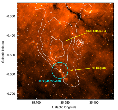
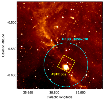
Figure 1: Left: region of about 30^′ $\times$ 30^′ towards SNR G35.6-0.4 presenting the emission at 8 $\mu$m with contours of the radio continuum emission at 20 cm. The contours levels are 17, 22, and 30 K. The first contour is slightly above the data 3$\sigma_{rms}$. The circle shows the position and the extension of HESS J1858+020. We remark the possibility that the SNR is partially superimposed over an HII region. Right: smaller portion of the region displaying the 8 $\mu$m emission and showing the area mapped with the molecular observations (yellow box).

4 Results and discussion

Figure 2: Up: ¹²CO J=3–2 spectra. Bottom: ¹³CO J=3–2 spectra. The horizontal axis of each spectra is velocity, and ranges from 30 to 80 km s^-1, while the vertical axis is brightness temperature and goes from -1 to 7 K. The center, i.e. the (0,0) offset, in both lines is the same.

Figure 2 (up) shows the ¹²CO J=3–2 spectra obtained towards the observed region. In the whole area the main component at $\sim$53 km s^-1, already detected in the ¹³CO J=1–0 clump studied by Paron & Giacani (2010), is present. A second, less intense, component is observed mainly towards positive RA and negative Dec offsets (bottom left in the image) with a velocity of $\sim$64 km s^-1. Note that, due to lack of observing time, three positions were not observed (top right of the image). Fig. 2 (bottom) displays the ¹³CO J=3–2 spectra observed towards the central $\sim$20 square arcseconds. In the observed area, this line has a unique component centered at $\sim$53 km s^-1. In both cases, the horizontal axis of each spectra is velocity and ranges from 30 to 80 km s^-1, while the vertical axis is brightness temperature and goes from -1 to 7 K. The ¹²CO J=3–2 component at $\sim$64 km s^-1 has no correspondence neither in the ¹³CO J=3–2 emission presented in this work, nor in the ¹³CO J=1–0 emission analyzed in Paron & Giacani (2010). We suggest that this velocity component can be unrelated molecular gas seen along the line of sight. In what follows, we focus our analysis on the $\sim$53 km s^-1 molecular component. Table 1 summarizes the derived parameters of the ¹²CO and ¹³CO J=3–2 lines obtained from a Gaussian fitting. T_mb is the main beam peak brightness temperature, V_LSR is the central velocity referred to the Local Standard of Rest and $\Delta v$ is the line width (FWHM). The Gaussian fitting was performed to the averaged spectrum of each line, which was obtained from the pointings within the area mapped by the ¹³CO emission, at the center of the region. The quoted uncertainties are formal 1$\sigma$ value for the model of the Gaussian shape.

Table 1: Parameters of the ¹²CO and ¹³CO J=3–2 lines from the center of the region.

Emission	Tmb	VLSR	$\Delta v$
	(K)	(km s-1)	(km s-1)
12CO J=3–2	10.50 $\pm$ 0.40	53.15 $\pm$ 0.22	2.60 $\pm$ 0.15
13CO J=3–2	5.20 $\pm$ 0.50	53.30 $\pm$ 0.15	2.00 $\pm$ 0.10

An inspection of the ¹²CO J=3–2 spectra indicates that there are not spectral wings nor intensity gradients along symmetric directions in the plane of the sky, which allows us to conclude that, at the present data resolution, there is not evidence of outflow activity neither in the plane of the sky nor along the line of sight. The detected molecular clump peaks approximately at the (10,0) offset (see Fig. 2), corresponding to the sky positon $l=$ 35$\aas@@fstack{\circ}$57, $b=-$0$\aas@@fstack{\circ}$58. Figure 3 displays a two color image with the 8 $\mu$m and 24 $\mu$m emissions in red and green, respectively, with contours of the ¹²CO J=3–2 emission integrated between 48 and 57 km s^-1. The circle represents the source HESS J1858+020. From this image it can be appreciated that the molecular clump mapped in ¹²CO J=3–2 coincides with the condensation of PAHs seen at 8 $\mu$m. This image reveals that such clump also emits at 24 $\mu$m indicating warm dust. The presence of this clump, lying exactly at the geometric center of the HESS source, suggests that its study may help to elucidate the nature of the high energy emission. It is important to note that we did not detect emission of the HCO⁺ J=4–3 and CS J=7–6 lines at a sensitivity levels of about 0.13 and 0.2 K, respectively in the direction to this molecular concentration.

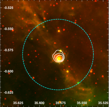
Figure 3: Two color image with the 8 $\mu$m and 24 $\mu$m emissions presented in red and green, respectively. The contours correspond to the ¹²CO J=3–2 emission integrated between 48 and 57 km s^-1, at the levels of 22, 26, and 30 K km s^-1. The rms noise is about 4 K km s^-1. The circle represents the extension of the source HESS J1858+020.

To estimate the physical parameters of the molecular clump we assume LTE conditions and a beam filling factor of 1, which may not be completely true but allow us to make a first approach to the problem. From the peak temperature ratio between the CO isotopes (¹²T_mb/¹³T_mb), it is possible to estimate the optical depths from (e.g. Curtis et al. 2010):

$$\frac{{}^{12}{\rm T}_{mb}}{{}^{13}{\rm T}_{mb}}=\left(\frac{\nu_{12}}{\nu_{13}}\right)^{2}\frac{[^{12}\rm{CO}]}{[^{13}\rm{CO}]}\frac{1-exp(-\tau_{12})}{\tau_{12}},$$

where $\nu_{12}=345.796$ GHz and $\nu_{13}=330.558$ GHz are the transition frequencies of ¹²CO and ¹³CO J=3–2 lines, respectively, $\tau_{12}$ is the optical depth of the ¹²CO gas and [¹²CO]/[¹³CO] is the isotope abundance ratio. Assuming 8 kpc as the distance to the galactic center and using [¹²CO]/[¹³CO] $=(6.21\pm 1.00){\rm D_{GC}}+(18.71\pm 7.37$) (Milam et al., 2005) where D${}_{\rm GC}=6.73$ kpc is the distance between the source and the galactic center, we obtain [¹²CO]/[¹³CO] $=56.7\pm 13.5$. Thus, the ¹²CO J=3–2 optical depth is $\tau_{12}=32\pm 11$. Using the typical LTE equations and taking into account that the ¹²CO J=3–2 line is optically thick as shown above, from its emission we estimate an excitation temperature of T${}_{\rm ex}=17\pm 1$ K. Using this factor and the ¹³CO J=3–2 emission, we derive an optical depth for the ¹³CO of $\tau^{13}=0.70\pm 0.12$ and a ¹³CO column density of N(¹³CO) $=(8.2\pm 1.2)\times 10^{15}$ cm^-2. Adopting the isotope abundance ratio [¹²CO]/[¹³CO] used above and the relationship of N(H₂)/N(¹²CO) $\sim 10^{4}$ (see Black & Willner 1984 and reference therein), we obtain an H₂ column density of N(H₂) $=(5.0\pm 1.8)\times 10^{21}$ cm^-2. Finally, assuming spherical geometry for the clump, compatible with what is seen in Fig. 3, with a radius of $\sim$30^′′ ($\sim$1.5 pc at the distance of 10.5 kpc), we estimate a mass and a volume density of $(1.5\pm 0.5)\times 10^{3}\times(\frac{d}{10.5\leavevmode\nobreak\ {\rm kpc}})^{2}$ M_⊙, and $(2.1\pm 0.7)\times 10^{3}\times(\frac{10.5\leavevmode\nobreak\ {\rm kpc}}{d})^{3}$ cm^-3, respectively for this structure, where $d$ is the distance. The quoted errors, of the order of 30%, do not include the error in the distance, which is a major unknown and depends on Galaxy models. We thus present the estimated values as a function of the distance.

On the other hand, using the ¹³CO line width of $\Delta v=2$ km s^-1 and a radius of $R=1.5$ pc, we calculate the virial mass from: M${}_{vir}=B\times R\times\Delta v^{2}$, where $B$ is a constant that depends on the density profile. If one assumes a uniform density profile, that is $\rho(r)=constant$, $B=210$, while if a density profile $\rho(r)\propto 1/r$ is assumed, $B=190$ (MacLaren et al., 1988). Both cases produce the same virial mass within the errors, M${}_{vir}=(1.1\pm 0.1)\times 10^{3}\times\frac{d}{10.5\leavevmode\nobreak\ {\rm kpc}}$ M_⊙. The ratio between the virial and the LTE mass is M_vir/M${}_{\rm{LTE}}=(0.8\pm 0.3)\times\frac{10.5\leavevmode\nobreak\ {\rm kpc}}{d}$. Kawamura et al. (1998) performed a large scale survey of molecular clouds towards the Gemini and Auriga regions and shows that star-forming ¹³CO clouds have low M_vir/M_LTE, while all the clouds with high M_vir/M_LTE have no sign of star formation. On the other hando, several molecular cores studied in the active stellar forming complex in Taurus have on average, M_vir/M${}_{\rm{LTE}}\sim 0.6$ (Onishi et al., 1996), quite similar to the 0.8 derived here.

Another way to estimate the volume density of the molecular feature is through the investigation of the dust content. Figure 4 displays the smoothed 1.1 mm continuum emission obtained from the BGPS (Aguirre et al., 2011) with the ¹²CO J=3–2 contours presented in Fig. 3. The crosses indicate the position of two sources from the BGPS catalog (Rosolowsky et al., 2010), showing that the analyzed molecular clump coincides with the source BGPS G035.578-00.584.

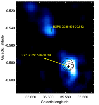
Figure 4: BGPS continuum emission at 1.1 mm with the ¹²CO J=3–2 contours presented in Fig. 3. The crosses indicate the position of two sources catalogued in the BGPS Catalog.

According to the BGPS Catalog, the source BGPS G035.578-00.584 has an integrated flux density at 1.1 mm of $S_{\nu}=0.37\pm 0.10$ Jy and an elliptical shape with a major and minor axis of 16$\aas@@fstack{\prime\prime}$9 and 13$\aas@@fstack{\prime\prime}$6, respectively. The total mass of gas and dust in a core is proportional to the total flux density $S_{\nu}$, assuming that the dust emission at 1.1 mm is optically thin and both the dust temperature and opacity are independent of position within the core (Enoch et al., 2006). We can then calculate the core mass from the BGPS G035.578-00.584 flux density using:

$$M=\frac{d^{2}S_{\nu}}{B_{\nu}(T_{d})\kappa_{\nu}},$$

where $\kappa_{1.1{\rm mm}}=0.0114$ cm² g^-1 is the dust opacity estimated on the basis of the canonical gas-to-dust mass ratio of 100 (Enoch et al., 2006), $d$ the distance, $B_{\nu}$ the Planck function, and $T_{d}$ the dust temperature. Although the millimeter emission arises only from the dust, it is possible to infer the total mass of gas and dust because, as mentioned above, the dust opacity $\kappa_{1.1{\rm mm}}$ contains the gas-to-dust mass ratio (see Enoch et al. 2006). Following Rosolowsky et al. (2010), the above equation can be written as:

$$M=13.1{\rm M_{\odot}}\left(\frac{d}{1{\rm kpc}}\right)^{2}\left(\frac{S_{\nu}}{1{\rm Jy}}\right)\left[\frac{exp(13/T_{d})-1}{exp(13/20)-1}\right].$$

Assuming a typical dust temperature of $T_{d}=20$ K and the distance of 10.5 kpc, we obtain a total mass for the core BGPS G035.578-00.584 of $M=(535\pm 15)\times(\frac{d}{10.5\leavevmode\nobreak\ {\rm kpc}})^{2}$ M_⊙. Finally, using this mass and assuming an angular radius of 14^′′ ($R\sim 0.7$ pc), from $n_{\rm{H}}=3M/(4\pi R^{3}\mu m_{\rm{H}})$, where $m_{\rm{H}}$ is the hydrogen atom mass and $\mu=2.37$ the mean particle mass, we obtain a particle density of $n_{\rm{H}}=(6.6\pm 0.2)\times 10^{3}\times(\frac{10.5\leavevmode\nobreak\ {\rm kpc}}{d})^{3}$ cm^-3. The adopted angular radius is based on the angular size of this object as reported in the catalog. As it can be appreciated, the minor axis size is smaller than the rms size of the BGPS beam, thus it is not possible to calculate the deconvolved angular radius following Rosolowsky et al. (2010).

In summary, from two different methods we obtain a density of a few $10^{3}$ cm^-3 for the studied clump. Taking into account the lack of emission of the CS J=7–6 and HCO⁺ J=4–3 lines, tracers of higher densities, we conclude that $10^{3}-10^{4}$ cm^-3 is a plausible range for the density in the clump.

4.1 Young stellar objects in the molecular clump

Paron & Giacani (2010) conducted a search for young stellar objects (YSOs) probably embedded in the molecular cloud mapped in the ¹³CO J=1–0 line. Using the color criteria of Allen et al. (2004) for GLIMPSE sources, the authors found six YSO candidate sources. In this work, we look for YSOs probably embedded in the discovered ¹²CO J=3–2 clump using criteria based on the intrinsic reddening of the sources and studying the physical parameters extracted from the YSOs spectral energy distributions (SEDs). These criteria are based in the fact that YSOs always show intrinsic infrared excess that cannot be attributed to scattering and/or absorption of the ISM along the line of sight. We therefore used the GLIMPSE Point-Source Catalog to search for this kind of sources within the molecular clump. Robitaille et al. (2008) defined a color criterion to identify intrinsically red sources using data from the Spitzer-IRAC bands. Intrinsically red sources satisfy the condition $m_{4.5}-m_{8.0}\geq 1$, where $m_{4.5}$ and $m_{8.0}$ are the magnitudes in the 4.5 and 8.0 $\mu$m bands, respectively. To consider the errors in the magnitudes, we use the following color criterion to select intrinsically red sources: $m_{4.5}-m_{8.0}+\varepsilon\geq 1$, where $\varepsilon=\sqrt{(\Delta_{4.5})^{2}+(\Delta_{8.0})^{2}}$ and $\Delta_{4.5}$ and $\Delta_{8.0}$ are the errors of the 4.5 and 8.0 $\mu$m bands, respectively. By inspecting a circular region of about 30^′′ in radius centered at $l=$ 35$\aas@@fstack{\circ}$578, $b=-$0$\aas@@fstack{\circ}$582, we find 27 GLIMPSE sources, and by applying the above mentioned color criterion, we find only two intrinsically red sources that appear to be related to the molecular clump, they are: SSTGLMC G035.5768-00.5862 and SSTGLMC G035.5765-00.5909, hereafter IRS1 and IRS2, respectively. These sources were classified as class I and II, respectively in Paron & Giacani (2010) following the Allen et al. (2004) classification. Now, in view of our more complete study, we suggest that IRS1 is very likely embedded in the analyzed molecular clump, while for IRS2, lying in the border of the observed region, the connection with the studied molecular feature is less compelling.

Table 2: Near- and mid-IR fluxes of IRS1 and IRS2.

Source	$J$	$H$	$K_{S}$	3.6 $\mu$m	4.5 $\mu$m	5.8 $\mu$m	8.0 $\mu$m	24 $\mu$m
	(mag)	(mag)	(mag)	(mag)	(mag)	(mag)	(mag)	(Jy)
IRS1	–	–	13.462	10.253	9.225	8.301	7.533	0.032
IRS2	15.318	13.344	12.342	10.731	10.137	9.625	9.053	0.150

In Table 2 we present the catalogued near- and mid-IR fluxes of these sources extracted from the 2MASS and GLIMPSE point source catalogs. The fluxes at 24 $\mu$m were obtained from the MIPS image. These fluxes were used to calculate the SED of IRS1 and IRS2 using the tool developed by Robitaille et al. (2006, 2007) and available online. To perform the SED we assume an interstellar absorption between 10 and 30 mag. The lower value is compatible with the rough assumption of 1 mag per kpc that is commonly used. The upper value is in agreement with the visual absorption obtained from $A_{v}=5\times{10^{-22}}N(H)$ (Bohlin et al., 1978), where N(H) $=$ N(HI)$+$2N(H₂) is the line-of-sight hydrogen column density towards this region, which we estimate in about 5.8 $\times 10^{22}$ cm^-2. This value was obtained from the HI column density derived from the VLA Galactic Plane Survey (VGPS) HI data (Stil et al., 2006) and from the H₂ column density derived above. In Table 3, we report the main results of the SED fit output for IRS1 and IRS2. In Col. 2 and 3 we report the $\chi^{2}$ of the YSO and stellar photosphere best-fit model, respectively. The remaining columns report the physical parameters of the source for the best-fit model: central source mass, disk mass, envelope mass, and envelope accretion rate, respectively. Figure 5-right shows the SED of these sources.

Table 3: Parameters derived from the SED fitting of sources IRS1 and IRS2.

Source	$\chi^{2}_{YSO}$	$\chi^{2}_{\star}$	M⋆	Mdisk	Menv	$\dot{M}_{env}$
			(M⊙)	(M⊙)	(M⊙)	(M${}_{\odot}/yr$)
IRS1	4.1	412	9.6	3.2 $\times 10^{-2}$	3.6 $\times 10^{-6}$	0
IRS2	4.6	166	6.4	3.3 $\times 10^{-2}$	1.7	5 $\times 10^{-6}$

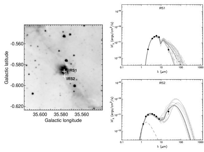
Figure 5: Left: Location of sources IRS1 and IRS2. Right: SED of these sources performed with the tool developed by Robitaille et al. (2006, 2007). Black line shows the best fit, and the gray lines show subsequent good fits. The dashed line shows the stellar photosphere corresponding to the central source of the best fit model, as it would look in the absence of circumstellar dust. The points are the input fluxes.

To relate the SED to the evolutionary stage of the YSO, Robitaille et al. (2006) defined three different stages based on the values of the central source mass M_⋆, the disk mass M_disk, and the envelope accretion rate $\dot{\rm M}_{env}$ of the YSO. Stage I YSOs are those that have $\dot{\rm M}_{env}$$/$M${}_{\star}>10^{-6}$ yr^-1, i.e., protostars with large accretion envelopes; stage II are those with M${}_{disk}/$M${}_{\star}>10^{-6}$ and $\dot{\rm M}_{env}$$/$M${}_{\star}<10^{-6}$ yr^-1, i.e., young objects with prominent disks; and stage III are those with M${}_{disk}/$M${}_{\star}<10^{-6}$ and $\dot{\rm M}_{env}$$/$M${}_{\star}<10^{-6}$ yr^-1, i.e. evolved sources where the flux is dominated by the central source. According to this classification, we conclude that IRS1 and IRS2 are stage II sources. However, IRS2 must be younger than IRS1 because, as can be appreciated in Table 3, it has a massive envelope which must still be accreting mass. The evolutionary stage of IRS1 derived from its SED and the lack of evidence of molecular outflows in the clump where it is embedded, suggest that IRS1 is an evolved YSO probably in the last stages of formation. Moreover, the presence of a condensation of PAH around this source suggests that IRS1 could be a high mass protostellar object (HMPO) that has not yet reached the ultracompact HII region stage.

4.2 The scenario

Based on the results presented above, in this section we discuss about the possible origin of the very-high energy emission.

As mentioned in Sec. 3 we propose that the SNR G35.6-0.4 is partially overlapping an extended HII region, whose eastern border is delineated by PAHs revealed through the 8 $\mu$m emission. A molecular cloud composed by at least two clumps lies over this border, and one of them is located at the center of HESS J1858+02. We have shown that there is at least one YSO embedded in such clump (that we called IRS1). Such object can, in principle, creates a population of ralativistic particles inside the host molecular cloud via a thermal jet. These particles, in a high density ambient matter can originate $\gamma-$ray emission through Inverse Compton and relativistic Bremsstrahlung losses (Araudo et al., 2007). However, in the case of IRS1, at the present data resolution, no evidence of molecular outflows has been found neither in the plane of the sky nor along the line of sight, therefore weakening the probability of a physical link between IRS1 and HESS J1858+020. Having demonstrated that the presence of a YSO in the molecular clump does not play a decisive role in the production of the observed $\gamma-$rays, and in view of the lack of any other candidate in the region at any distance, we are led to the conslusion that the only possible Galactic counterpart for the HESS source is the SNR G35.6-0.4 with its molecular enviroment. In this case, the supernova shock is a source of accelerated cosmic rays and the dense molecular clump provides the nuclei responsible for the production of neutral pions (through inelastic pp collisions) which will decay yielding the observed $\gamma-$rays.

5 Summary

Using molecular observations obtained with the Atacama Submillimeter Telescope Experiment (ASTE) and IR and submillimeter continuum archival data, we study a molecular clump associated with the IR source IRAS 18558+0201 that lies at the center of the very-high energy source HESS J1858+020. The main results can be summarized as follows:

(a) From the ¹²CO and ¹³CO J=3–2 lines and the 1.1 mm continuum emission we derived for this clump a density between $10{{}^{3}}$ and $10{{}^{4}}$ cm^-3. This clump is part of a larger molecular cloud that is being disturbed by the SNR G35.6-0.4 and by a nearby extended HII region.

(b) From the analysis of the mid-IR data and a photometric study we discovered a YSO very likely embedded in the mentioned molecular clump. Analyzing its spectral energy distribution we suggest that this source could be a high mass protostellar object that has not reached the ultracompact HII region stage.

(c) We did not find any evidence of molecular outflows from the discovered YSO that would reveal the presence of a thermal jet capable by itself of generating the very-high energy emission.

(d) We conclude that the presence of a clumpy molecular cloud, like the one investigated in this work, is the most plausible explanation for the very-high energy emission. The molecular gas may be acting as a target for the cosmic rays accelerated by the shock front of the SNR G35.6-0.4 generating the $\gamma-$ray emission through hadronic processes.