Measurement of exclusive production of scalar $\chi_{c0}$ meson
in proton-(anti)proton collisions via $\chi_{c0}\to\pi^{+}\pi^{-}$ decay

Abstract

We consider a measurement of exclusive production of scalar $\chi_{c}(0^{++})$ meson in the proton-proton collisions at LHC and RHIC and in the proton-antiproton collisions at the Tevatron via $\chi_{c0}\to\pi^{+}\pi^{-}$ decay. The corresponding amplitude for exclusive double-diffractive $\chi_{c0}$ meson production was obtained within the $k_{t}$-factorization approach including virtualities of active gluons and the corresponding cross section is calculated with unintegrated gluon distribution functions (UGDFs) known from the literature. The four-body $pp\to pp\pi^{+}\pi^{-}$ reaction constitutes an irreducible background to the exclusive $\chi_{c0}$ meson production. We calculate several differential distributions for $pp(\bar{p})\to pp(\bar{p})\chi_{c0}$ process including absorptive corrections. The influence of kinematical cuts on the signal-to-background ratio is investigated. Corresponding experimental consequences are discussed.

I Introduction

The mechanism of exclusive production of mesons at high energies became recently a very active field of research (see e.g. Ref. ACF10 and references therein). Central exclusive production processes represent a very promising and novel way to study QCD in hadron-hadron collisions. Recently, there is a growing interest in understanding exclusive three-body reactions $pp\to ppM$ at high energies, where the meson (resonance) $M$ is produced in the central rapidity region. In particular, these reactions provide a valuable tool to investigate in detail the properties of resonance states. Many of the resonances decay into $\pi\pi$ and/or $KK$ channels. The representative examples are: $M=\sigma,\rho^{0},f_{0}(980),\phi,f_{2}(1275),f_{0}(1500)$ and, as we shall emphasis here, $\chi_{c0}$. Various decay channels can be studied. It is clear that these resonances are seen (or will be seen) ”on” the background of a $\pi\pi$ or $KK$ continuum . The two-pion background to exclusive production of $f_{0}(1500)$ meson was already discussed in Ref. SL09 . The recent works concentrated on the production of $\chi_{c}$ mesons (see e.g. Refs. PST_chic0 ; PST_chic1 ; PST_chic2 ; LKRS10 ; LKRS11 and references therein) where the QCD mechanism is similar to the exclusive production of the Higgs boson. Furthermore, the $\chi_{c(0,2)}$ states are expected to annihilate via two-gluon processes into light mesons and may, therefore, allow the study of glueball production dynamics glueballs .

Recently, the CDF Collaboration has measured the cross section for exclusive production of $\chi_{c}$ mesons in proton-antiproton collisions at the Tevatron CDF_chic , by selecting events with large rapidity gaps separating the centrally produced state from the dissociation products of the incoming protons. In this experiment $\chi_{c}$ mesons are identified via decay to the $J/\psi+\gamma$ with $J/\psi\to\mu^{+}\mu^{-}$ channel. The experimental invariant mass resolution was not sufficient to distinguish between scalar, axial and tensor $\chi_{c}$. While the branching fractions to this channel for axial and tensor mesons are large PDG ($\mathcal{B}=(34.4\pm 1.5)\%$ and $\mathcal{B}=(19.5\pm 0.8)\%$, respectively) the branching fraction for the scalar meson is very small $\mathcal{B}=(1.16\pm 0.08)\%$ PDG . On the other hand, the cross section for exclusive $\chi_{c0}$ production obtained within the $k_{t}$-factorization is much bigger than that for $\chi_{c1}$ and $\chi_{c2}$. As a consequence, all $\chi_{c}$ mesons give similar contributions PST_chic2 to the $J/\psi+\gamma$ decay channel. Clearly, the measurement via decay to the $J/\psi+\gamma$ channel cannot provide cross section for different $\chi_{c}$.

Could other decay channels be used? The $\chi_{c0}$ meson decays into several two-body channels (e.g. $\pi\pi$, $K^{+}K^{-}$, $p\bar{p}$) or four-body hadronic modes (e.g. $\pi^{+}\pi^{-}\pi^{+}\pi^{-}$, $\pi^{+}\pi^{-}K^{+}K^{-}$). The branching ratios are shown in Table 1. In this paper we analyze a possibility to measure $\chi_{c0}$ via its decay to $\pi^{+}\pi^{-}$ channel. The advantage of this channel is that the $\pi^{+}\pi^{-}$ continuum has been studied recently LS10 and is relatively well known. In addition the axial $\chi_{c1}$ does not decay to the $\pi\pi$ channel and the branching ratio for the $\chi_{c2}$ decay into two pions is smaller. A much smaller cross section for $\chi_{c2}$ production means, in practice, that only $\chi_{c0}$ will contribute to the signal.

Table 1: Branching fractions for the $\chi_{cJ}$ two- and four-body hadronic decays, taken from Ref. PDG .

Channel	$\mathcal{B}(\chi_{c0})$	$\mathcal{B}(\chi_{c1})$	$\mathcal{B}(\chi_{c2})$
$\pi^{+}\pi^{-}$	$(0.56\pm 0.03)\times 10^{-2}$	$-$	$(0.16\pm 0.01)\times 10^{-2}$
$K^{+}K^{-}$	$(0.610\pm 0.035)\times 10^{-2}$	$-$	$(0.109\pm 0.008)\times 10^{-2}$
$p\bar{p}$	$(2.28\pm 0.13)\times 10^{-4}$	$(0.73\pm 0.04)\times 10^{-4}$	$(0.72\pm 0.04)\times 10^{-4}$
$\pi^{+}\pi^{-}\pi^{+}\pi^{-}$	$(2.27\pm 0.19)\times 10^{-2}$	$(0.76\pm 0.26)\times 10^{-2}$	$(1.11\pm 0.11)\times 10^{-2}$
$\pi^{+}\pi^{-}K^{+}K^{-}$	$(1.80\pm 0.15)\times 10^{-2}$	$(0.45\pm 0.10)\times 10^{-2}$	$(0.92\pm 0.11)\times 10^{-2}$

In the present paper, we wish to calculate differential distributions for the exclusive production $\chi_{c0}$ meson with a few UGDFs taken from the literature relevant for small gluon virtualities (transverse momenta). We shall use matrix element for the off-shell gluons as obtained in Ref. PST_chic0 . The expected non-resonant background can be modeled using a ”non-perturbative” framework, mediated by pomeron-pomeron fusion with an intermediate off-shell pion exchanged between the final-state particle pairs. Thus, we consider $pp(\bar{p})\to pp(\bar{p})\pi^{+}\pi^{-}$ reaction as a genuine four-body process with exact kinematics which can be easily used when kinematical cuts have to be improved.

Exclusive charmonium decays have been a subject of interest at the $e^{+}e^{-}$ colliders as they are an excellent laboratory for studying quark-gluon dynamics at relatively low energies. Thus, a measurement of many exclusive hadronic $\chi_{c}$ decays if possible is very valuable. Although these $\chi_{c}$ states are not directly produced in $e^{+}e^{-}$ collisions, they are copiously produced in the radiative decays $\psi(2S)\to\gamma\chi_{c}$, each of which has a branching ratio of around 9% PDG . The CLEO Collaboration has studied exclusive $\chi_{c(0,1,2)}$ decays to four-hadron final states involving two charged and two neutral mesons CLEO : $\pi^{+}\pi^{-}\pi^{0}\pi^{0}$, $K^{+}K^{-}\pi^{0}\pi^{0}$, $p\bar{p}\pi^{0}\pi^{0}$, $K^{+}K^{-}\eta\pi^{0}$ and $K^{\pm}\pi^{\mp}K^{0}\pi^{0}$. The BESIII Collaboration has studied two-body $\chi_{c(0,2)}$ decays into $\pi^{0}\pi^{0}$ and $\eta\eta$ BES_pi0pi0_etaeta and four-body $\chi_{c(0,1,2)}$ decays into $\pi^{0}\pi^{0}\pi^{0}\pi^{0}$ BES_4pi0 final states, where $\chi_{cJ}$ signals appear in radiative photon energy spectrum. Recently (Ref. BES_ppKK ) a study of $\chi_{cJ}$ hadronic decays and measurements of $\chi_{cJ}\to\Lambda(1520)\bar{\Lambda}(1520)$ decaying into $p\bar{p}K^{+}K^{-}$ has been presented. In the present paper we start the discussion of the possibility to measure the different decay channels in proton-(anti)proton collisions in order to determine the cross section for exclusive production of the P-wave charmonia. Here, continuum backgrounds can be larger than in the $e^{+}e^{-}$ collisions and this requires a separate discussion of the feasibility. We will discuss this issue in the present paper.

The paper is organized as follows. In section II we give general expressions for the amplitudes of the exclusive $\chi_{c0}$ meson production and $\pi^{+}\pi^{-}$ pairs production including discussion of absorptive corrections. Section III contains the presentation of the main results and a discussion of the uncertainties related to the approximations made. Finally, some concluding remarks and outlook are given in Section IV.

II Signal and background amplitudes

II.1 Diffractive QCD amplitude for exclusive $\chi_{c0}$ production

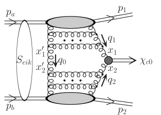
Figure 1: The QCD mechanism of exclusive diffractive production of $\chi_{c0}$ meson including the absorptive correction.

The QCD mechanism for the diffractive production of heavy central system has been proposed by Khoze, Martin and Ryskin (KMR) and developed in collaboration with Kaidalov and Stirling for Higgs production (see e.g. Refs. KMR ; KKMR ; KKMR-spin ; KMRS ). In the framework of this approach the amplitude of the exclusive $pp\to pp\chi_{c0}$ process is described by the diagram shown in Fig. 1, where the hard subprocess $g^{*}g^{*}\to\chi_{c0}$ is initiated by the fusion of two off-shell gluons and the soft part represented in terms of the off-diagonal unintegrated gluon distributions (UGDFs). The formalism used to calculate the exclusive $\chi_{c0}$ meson production is explained in detail elsewhere PST_chic0 and so we will only review relevant aspects here.

The ”full” amplitude for the exclusive process $pp\to pp\chi_{c0}$ can be written as

$${\cal{M}}_{pp\to pp\chi_{c}}^{full}(s,y,-\mbox{\boldmath$p$}_{1,t},-\mbox{\boldmath$p$}_{2,t}) = {\cal{M}}_{pp\to pp\chi_{c}}^{bare}(s,y,-\mbox{\boldmath$p$}_{1,t},-\mbox{\boldmath$p$}_{2,t})$$ (1)

$$+ {\cal{M}}_{pp\to pp\chi_{c}}^{rescatt}(s,y,-\mbox{\boldmath$p$}_{1,t},-\mbox{\boldmath$p$}_{2,t})\,.$$

We can write the ”bare” amplitude PST_chic0 as

$${\cal M}_{pp\to pp\chi_{c}}^{bare}(s,y,-\mbox{\boldmath$p$}_{1,t},-\mbox{\boldmath$p$}_{2,t})=$$

$$\frac{s}{2}\pi^{2}\frac{1}{2}\frac{1}{N_{c}^{2}-1}\Im\int d^{2}q_{0,t}V(\mbox{\boldmath$q$}_{1,t},\mbox{\boldmath$q$}_{2,t})\frac{f^{off}_{g1}(x_{1},x^{\prime},q_{0,t}^{2},q_{1,t}^{2},t_{1})f^{off}_{g2}(x_{2},x^{\prime},q_{0,t}^{2},q_{2,t}^{2},t_{2})}{q_{0,t}^{2}\,q_{1,t}^{2}\,q_{2,t}^{2}}\,,$$ (2)

where the objects $f_{g1/g2}^{off}$ are skewed (or off-diagonal) unintegrated gluon distributions of both nucleons. $t_{1,2}$ are the momentum transfers along each nucleon line , $q_{1,t}$, $q_{2,t}$, $q_{0,t}$, $x_{1,2}$, $x^{\prime}_{1}\sim x^{\prime}_{2}\ll x_{1,2}$ are the transverse momenta and the longitudinal momentum fractions for active and screening gluons, respectively. UGDFs are nondiagonal both in the $x$ and $q_{t}^{2}$ space. The usual off-diagonal gluon distributions are nondiagonal only in $x$. In the limit $x_{1,2}\to x^{\prime}_{1,2}$, $q_{0,t}^{2}\to q_{1/2,t}^{2}$ and $t_{1,2}\to 0$ they become the usual UGDFs.

The vertex factor $V(\mbox{\boldmath$q$}_{1,t},\mbox{\boldmath$q$}_{2,t})$ describes the coupling of two virtual gluons to $\chi_{c0}$ meson is obtained in heavy quark approximation and can be written as

$$V(\mbox{\boldmath$q$}_{1,t},\mbox{\boldmath$q$}_{2,t})=K_{NLO}\frac{8ig_{s}^{2}}{M}\frac{{\cal R}^{\prime}(0)}{\sqrt{\pi MN_{c}}}\frac{3M^{2}\mbox{\boldmath$q$}_{1,t}\mbox{\boldmath$q$}_{2,t}-2\mbox{\boldmath$q$}_{1,t}^{2}\mbox{\boldmath$q$}_{2,t}^{2}-(\mbox{\boldmath$q$}_{1,t}\mbox{\boldmath$q$}_{2,t})(\mbox{\boldmath$q$}_{1,t}^{2}+\mbox{\boldmath$q$}_{2,t}^{2})}{(M^{2}+\mbox{\boldmath$q$}_{1,t}^{2}+\mbox{\boldmath$q$}_{2,t}^{2})^{2}}\,,$$ (3)

where $M$ is the $\chi_{c0}$ mass, $g_{s}^{2}=4\pi\alpha_{s}(M^{2})$ and the strong coupling constant is calculated in the leading order and extended to the nonperturbative region according to Shirkov-Solovtsov analytical model SS97 . The value of the $P$-wave radial wave function at the origin is taken to be EQ95 ${\cal R}_{\chi_{cJ}}^{\prime}(0)=\sqrt{0.075}$ GeV^5/2 and the radiative corrections factor in the vertex $K_{NLO}$ is well-known KNLO , $K_{NLO}\simeq 1.68$.

The rescattering correction shown in Fig. 1 by the extra blob can be written in the form

$${\cal M}_{pp\to pp\chi_{c}}^{rescatt}(s,y,-\mbox{\boldmath$p$}_{1,t},-\mbox{\boldmath$p$}_{2,t}) = \int\frac{d^{2}\mbox{\boldmath$k$}_{t}}{2(2\pi)^{2}}\frac{A_{pp}(s,k_{t}^{2})}{s}{\cal M}_{pp\to pp\chi_{c}}^{bare}(s,y,\mbox{\boldmath$k$}_{1,t},\mbox{\boldmath$k$}_{2,t})\,,$$ (4)

where $\mbox{\boldmath$k$}_{1,t}=-\mbox{\boldmath$p$}_{1,t}-\mbox{\boldmath$k$}_{t}$ and $\mbox{\boldmath$k$}_{2,t}=-\mbox{\boldmath$p$}_{2,t}-\mbox{\boldmath$k$}_{t}$ with momentum transfer $\mbox{\boldmath$k$}_{t}$. The amplitude for elastic proton-proton scattering at an appropriate energy is conveniently parameterized as

$$A_{pp}(s,k_{t}^{2}) = A_{0}(s)\,\exp(-Bk_{t}^{2}/2)\,.$$ (5)

From the optical theorem we have Im$A_{0}(s,t=0)=s\sigma_{tot}(s)$ (the real part is small in the high energy limit). $B$ is the effective slope of the elastic differential cross section

$$B(s)=B_{i}+2\alpha^{\prime}_{i}\ln\left(\frac{s}{s_{0}}\right)\,,$$ (6)

and is adjusted to the existing experimental data for the elastic $NN$ scattering. The Donnachie-Landshoff parametrization DL92 of the total $pp$ or $p\bar{p}$ cross sections can be used to calculate the rescattering amplitude. We take $s_{0}$ = 1 GeV², $\alpha^{\prime}_{I\!\!P}$ = 0.25 GeV^-2 and $B_{i}$: $B^{NN}_{I\!\!P}$ = 9 GeV^-2.

The KMR UGDFs, unintegrated over $q_{t}$, are calculated from the conventional (integrated) distributions $g(x,q_{t}^{2})$ and the so-called Sudakov form factor $\sqrt{T_{g}(q_{t}^{2},\mu^{2})}$ as follows:

$$f_{g}^{KMR}(x,x^{\prime},Q_{t}^{2},\mu^{2};t)=R_{g}\frac{\partial}{\partial\ln q_{t}^{2}}\left[xg(x,q_{t}^{2})\sqrt{T_{g}(q_{t}^{2},\mu^{2})}\right]_{q_{t}^{2}=Q_{t}^{2}}F(t)\,.$$ (7)

The Sudakov factor suppresses real emissions from the active gluon during the evolution, so that the rapidity gaps survive. The factor $R_{g}$ approximately accounts for the single $\mathrm{ln}Q_{t}^{2}$ skewed effect SGBMR99 . In the calculations presented here we take $R_{g}=1.3$, and value of the hard scale is $\mu^{2}=M^{2}/4$. The choice of the scale is somewhat arbitrary, and consequences of this choice were discussed in Ref. PST_chic0 .

In the original KMR approach the following prescription for the effective transverse momentum is taken:

$$Q_{1,t}^{2}=\mathrm{min}\left(q_{0,t}^{2},q_{1,t}^{2}\right)\,,\qquad Q_{2,t}^{2}=\mathrm{min}\left(q_{0,t}^{2},q_{2,t}^{2}\right)\,.$$ (8)

Other prescriptions are also possible PST_chic0 ; PST_chic1 . In the KMR approach only one effective gluon transverse momentum is taken explicitly in their skewed UGDFs compares to two independent transverse momenta in our case (see Eq. (2)). Please note also that the skewed KMR UGDFs does not explicitly depend on $x^{\prime}$ (assuming $x^{\prime}\ll x\ll 1$).

In Ref. MR01 a procedure was presented which allows to calculate the generalized (or skewed) parton distributions of the proton, $\overline{H}(x,\xi;q_{t}^{2},\mu^{2})$, unintegrated over the partonic transverse momenta, from the conventional parton distributions, $q(x,\mu^{2})$ and $g(x,\mu^{2})$, for small values of the skewedness parameter $\xi^{2}\ll 1$ and any $x$. The momentum fractions carried by the emitted and absorbed partons are defined as $x_{1,2}=x\pm\frac{1}{2}\xi$ with support $-1\leq x\leq 1$. The result is a simple approximate phenomenological form for the distribution:

$$\overline{H}_{g}\left(\frac{\xi}{2},\xi;q_{t}^{2},\mu^{2}\right) = \sqrt{T_{g}(q_{t}^{2},\mu^{2})}\left[R_{g}\>\frac{\partial xg(x,q_{t}^{2})}{\partial\ln q_{t}^{2}}\>+\>xg(x,q_{t}^{2})\>\frac{N_{c}\alpha_{s}}{2\pi}\left(\ln\frac{\mu+\frac{1}{2}q_{t}}{q_{t}}\>+\>1.2\frac{\mu^{2}}{\mu^{2}+q_{t}^{2}}\right)\right.$$ (9)

$$+\;5\left.\frac{\alpha_{s}}{2\pi}\left(xu_{\rm val}(x,q_{t}^{2})+xd_{\rm val}(x,q_{t}^{2})\right)\right]_{x=\xi}\,.$$

In evaluating $f_{g}$’s we have used the GRV NLO GRV and GJR NLO GJR collinear gluon distributions, which allow to use rather low values of gluon transverse momenta $Q_{t}^{2}=q_{0,t}^{2}$, $q_{1,t}^{2}$, $q_{2,t}^{2}\geq$ 0.5 GeV². The collinear distributions such as CTEQ and MRST are defined for higher factorization scales ($Q_{t}^{2}>1$ GeV²), and therefore are less useful in applications discussed here.

The $t$-dependence of the unintegrated gluon distribution $f_{g}$’s is not well known and is isolated in the effective form factors of the QCD Pomeron-proton vertex, which are parameterized in the forward scattering limit in the exponential form as

$$F(t)=\exp(b\,t/2)$$ (10)

with the $t$-slope parameter $b=4$ GeV^-2. Then the integral in Eq. (4) can be evaluated as KMR_eik

$${\cal M}_{pp\to pp\chi_{c}}^{rescatt}(s,y,-\mbox{\boldmath$p$}_{1,t},-\mbox{\boldmath$p$}_{2,t})=\frac{iA_{0}}{4\pi s(B+2b)}\exp\left(\frac{b^{2}|\mbox{\boldmath$p$}_{1,t}-\mbox{\boldmath$p$}_{2,t}|^{2}}{2(B+2b)}\right){\cal M}_{pp\to pp\chi_{c}}^{bare}(s,y,-\mbox{\boldmath$p$}_{1,t},-\mbox{\boldmath$p$}_{2,t})\,.$$

(11)

The cross section for the three-body reaction is calculated as

$$\sigma=\int\frac{1}{2s}\overline{|{\cal M}|^{2}}(2\pi)^{4}\delta^{4}(p_{a}+p_{b}-p_{1}-p_{2}-p_{3})\frac{d^{3}p_{1}}{(2\pi)^{3}2E_{1}}\frac{d^{3}p_{2}}{(2\pi)^{3}2E_{2}}\frac{d^{3}p_{3}}{(2\pi)^{3}2E_{3}}\;$$ (12)

by choosing convenient kinematical variables.

II.2 Diffractive amplitude for $\pi^{+}\pi^{-}$ continuum

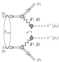
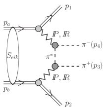
Figure 2: The double-diffractive mechanism of exclusive production of $\pi^{+}\pi^{-}$ pairs including the absorptive corrections.

The dominant mechanism of the exclusive production of $\pi^{+}\pi^{-}$ pairs at high energies is sketched in Fig. 2. In calculations of the amplitude related to double diffractive mechanism for the $pp\to pp\pi^{+}\pi^{-}$ reaction we follow the general rules of Pumplin and Henyey PH76 used recently in Ref. LS10 .

The ”full” amplitude for the exclusive process $pp\to pp\pi^{+}\pi^{-}$ (with four-momenta $p_{a}+p_{b}\rightarrow p_{1}+p_{2}+p_{3}+p_{4}$) can be written formally as

$${\cal{M}}_{pp\to pp\pi\pi}^{full}(s,y_{3},y_{4},\mbox{\boldmath$p$}_{1,t},\mbox{\boldmath$p$}_{2,t},\mbox{\boldmath$p$}_{m}) = {\cal{M}}_{pp\to pp\pi\pi}^{bare}(s,y_{3},y_{4},\mbox{\boldmath$p$}_{1,t},\mbox{\boldmath$p$}_{2,t},\mbox{\boldmath$p$}_{m})$$

$$+ {\cal{M}}_{pp\to pp\pi\pi}^{rescatt}(s,y_{3},y_{4},\mbox{\boldmath$p$}_{1,t},\mbox{\boldmath$p$}_{2,t},\mbox{\boldmath$p$}_{m})\,,$$

where the auxiliary quantity $\mbox{\boldmath$p$}_{m}=\mbox{\boldmath$p$}_{3,t}-\mbox{\boldmath$p$}_{4,t}$.

The ”bare” amplitude can be written as

$$\mathcal{M}_{pp\to pp\pi\pi}^{bare} = M_{13}(t_{1},s_{13})F_{\pi}(t_{a})\frac{1}{t_{a}-m_{\pi}^{2}}F_{\pi}(t_{a})M_{24}(t_{2},s_{24})$$ (14)

$$+ M_{14}(t_{1},s_{14})F_{\pi}(t_{b})\frac{1}{t_{b}-m_{\pi}^{2}}F_{\pi}(t_{b})M_{23}(t_{2},s_{23})\;,$$

where $M_{ik}$ denotes ”interaction” between nucleon $i=1$ (forward nucleon) or $i=2$ (backward nucleon) and one of the two pions $k=3$ ($\pi^{+}$), $k=4$ ($\pi^{-}$). The energy dependence of the amplitudes of the $\pi N$ subsystems was parameterized in the Regge form with pomeron and reggeon exchanges. The details of the matrix element are explained in Ref. LS10 . The strength parameters and values of the pomeron and reggeon trajectories are taken from the Donnachie-Landshoff analysis DL92 of the total cross section for $\pi N$ scattering. The slope parameters of the elastic $\pi N$ scattering can be written as shown in Eq. (6) and are $B_{I\!\!P}^{\pi N}$ = 5.5 GeV^-2, $B_{I\!\!R}^{\pi N}$ = 4 GeV^-2 LS10 , for pomeron and reggeon exchanges, respectively.

The Donnachie-Landshoff parametrization DL92 can be used only for the $\pi N$ subsystem energy $W_{ik}>2-3$ GeV (see Ref. LS10 ). Bellow $W_{ik}=2$ GeV the resonance states in $\pi N$ subsystems are present. In principle, their contribution could and should be included explicitly . In order to exclude resonance regions we shall ”correct” the parametrization (Eq. (14)) multiplying it by a purely phenomenological smooth cut-off correction factor LS10

$$f_{cont}^{\pi N}(W_{ik})=\frac{\exp\left(\frac{W_{ik}-W_{0}}{a}\right)}{1+\exp\left(\frac{W_{ik}-W_{0}}{a}\right)}\;.$$ (15)

The parameter $W_{0}=2$ GeV gives the position of the cut, and the parameter $a=0.2$ GeV describes how sharp the cut-off is. For large energies $f_{cont}^{\pi N}(W_{ik})\approx 1$ and close to kinematical threshold $f_{cont}^{\pi N}(W_{ik}\simeq m_{\pi}+m_{N})\approx 0$.

The extra form factors $F(t_{a})$ and $F(t_{b})$ ”correct” for off-shellness of the intermediate pions in the middle of the diagrams shown in Fig. 2. In the following they are parameterized as

$$F_{\pi}(t_{a,b})=\exp\left(\frac{t_{a,b}-m_{\pi}^{2}}{\Lambda^{2}_{off,E}}\right)\;,$$ (16)

i.e. normalized to unity on the pion-mass-shell. In general, the parameter $\Lambda_{off,E}$ is not known precisely but, in principle, could be fitted to the (normalized) experimental data. From our general experience in hadronic physics we expect $\Lambda_{off,E}^{2}\sim 1.2-2$ GeV². How to extract $\Lambda_{off,E}$ will be discussed in the result section.

The absorptive corrections to the ”bare” amplitude (Eq. (14)) can be written as:

$${\cal M}_{pp\to pp\pi\pi}^{rescat}=\mathrm{i}\int\frac{d^{2}\mbox{\boldmath$k$}_{t}}{2(2\pi)^{2}}\frac{A_{pp}(s,k_{t}^{2})}{s}{\cal M}_{pp\to pp\pi\pi}^{bare}(\mbox{\boldmath$p$}^{\,*}_{a,t}-\mbox{\boldmath$p$}_{1,t},\mbox{\boldmath$p$}^{\,*}_{b,t}-\mbox{\boldmath$p$}_{2,t})\;,$$ (17)

where $p^{\,*}_{a}=p_{a}-k_{t}$, $p^{\,*}_{b}=p_{b}+k_{t}$.

The amplitude described above (see Eq. LABEL:amp_pipi_full) is used to calculate the corresponding cross section including limitations of the four-body phase-space. The cross section for the two-pion continuum is obtained by integration over the four-body phase space:

$$\sigma=\int\frac{1}{2s}\overline{|{\cal M}|^{2}}(2\pi)^{4}\delta^{4}(p_{a}+p_{b}-p_{1}-p_{2}-p_{3}-p_{4})\frac{d^{3}p_{1}}{(2\pi)^{3}2E_{1}}\frac{d^{3}p_{2}}{(2\pi)^{3}2E_{2}}\frac{d^{3}p_{3}}{(2\pi)^{3}2E_{3}}\frac{d^{3}p_{4}}{(2\pi)^{3}2E_{4}}.$$

(18)

In order to calculate the total cross section one has to calculate the eight-dimensional integral numerically. The details how to conveniently reduce the number of kinematical integration variables are given elsewhere LS10 .

III Results

Let us start from presenting various differential cross sections. In practical integrations of the exclusive $\chi_{c0}$ meson we choose the transverse momenta of outgoing nucleons $(p_{1,t},p_{2,t})$, the meson rapidity $(y)$ and the relative azimuthal angle between outgoing nucleons $(\phi_{12})$.

In Fig. 3 we show distributions of the central exclusive $\chi_{c0}$ production cross section at $\sqrt{s}$ = 14 TeV without (dashed line) and with (solid line) absorptive corrections as described in subsection II.1. These calculations were done with GJR NLO GJR collinear gluon distribution, to generate the KMR UGDFs (see Eq. (7)), which allows to use low values of the gluon transverse momenta $Q_{t}^{2}\geq Q_{cut}^{2}=0.5$ GeV². The bigger the value of the cut-off parameter, the smaller the cross section (see Ref. PST_chic0 ). In the calculations we take the value of the hard scale to be $\mu^{2}=M^{2}/4$. The smaller $\mu^{2}$, the bigger the cross section PST_chic0 . The absorption effects lead to a damping of the cross section. In most distributions the shape is almost unchanged. Exception is the distribution in proton transverse momentum where the absorption effects lead to a damping of the cross section at small proton $p_{t}$ and an enhancement of the cross section at large proton $p_{t}$. In relative azimuthal angle distribution we observe a ”diffractive dip” structure in the region of $\phi_{12}\sim\pi/2$. Transverse momentum distribution of $\chi_{c0}$ shows a small minimum at $p_{t}\sim$ 2.5 GeV. The main reason of its appearance is the functional dependence of matrix elements on its arguments PST_chic0 .

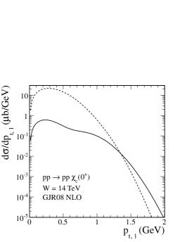
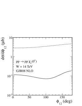
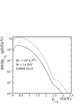
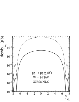
Figure 3: Differential cross sections for the $pp\to pp\chi_{c0}$ reaction at $\sqrt{s}$ = 14 TeV without (dashed line) and with (solid line) absorption effects. These calculations were done with the GJR08 NLO GJR UGDFs.

In Fig. 4 we compare distributions of the central exclusive $\chi_{c0}$ production cross section at $\sqrt{s}$ = 14 TeV calculated for two collinear gluon distributions: GRV94 NLO (upper lines) and GJR08 NLO (bottom lines). We show results here only for distributions with absorptive corrections calculated with the KMR off-diagonal UGDFs given by Eq. (7) (solid lines) and with off-diagonal UGDFs given in the phenomenological form given by Eq. (9). The peaks at large rapidities appear only when we use formula (7). In this region one of off-diagonal UGDFs changes a sign. This shows limitations in applying formula (7).

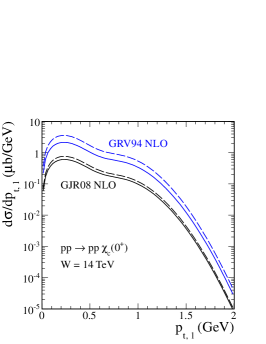
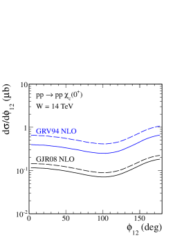
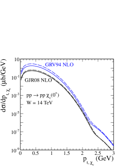
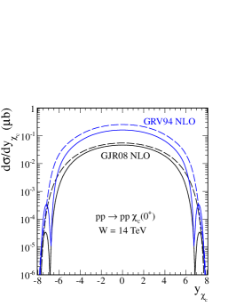
Figure 4: Differential cross sections for the $pp\to pp\chi_{c0}$ reaction at $\sqrt{s}$ = 14 TeV with absorption effects. The results with KMR off-diagonal UGDFs given by Eq. (7) (solid lines) and with off-diagonal UGDFs given by Eq. (9) (dashed lines) are shown. These calculations were done for two UGDFs: GRV94 NLO (upper lines) and GJR08 NLO (bottom lines).

Let us turn now to an estimation of the two-pion background. In Fig. 5 we show the two-pion invariant mass distribution at the center-of-mass energy of the CERN ISR $\sqrt{s}=62$ GeV (this is the highest energy at which experimental data exist). Here we have used a simple model described in subsection II.2. The experimental cuts on the rapidity of both pions and on longitudinal momentum fractions (Feynman-$x$, $x_{F}=2p_{\parallel}/\sqrt{s}$) of both outgoing protons are included when comparing our results with existing experimental data from ABCDHW90 (see Refs. WSW83 ; ABCDHW89 for early studies). Absorption effects were included in this calculation. The results depend on the value of the nonperturbative, a priori unknown parameter of the form factor responsible for off-shell effects (see Eq. (16)). We show results with the cut-off parameters $\Lambda_{off,E}^{2}=1.6,1.8,2.0$ GeV² as represented by the dotted, dashed and solid line, respectively. The experimental data show some peaks above our flat model continuum. They correspond to the well known $\pi^{+}\pi^{-}$ resonances: $\sigma$, $\rho^{0}$, $f_{2}(1275)$ which are not included explicitly in our calculation. In the present analysis we are interested mostly what happens above $M_{\pi\pi}>3$ GeV, above the resonance region where there are no experimental data points. Our model with $\Lambda_{off,E}$ parameter fitted to the data provides an educated extrapolation to the unmeasured region.

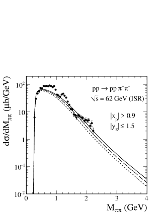
Figure 5: Differential cross section $d\sigma/dM_{\pi\pi}$ for the $pp\to pp\pi^{+}\pi^{-}$ reaction at $\sqrt{s}=62$ GeV with experimental cuts relevant for the CERN ISR experimental data from Ref. ABCDHW90 . Results with the cut-off parameters $\Lambda_{off,E}^{2}=1.6,1.8,2.0$ GeV² are shown by the dotted, dashed and solid line, respectively. The absorption effects were included in the calculations.

In Fig. 6 we show differential distributions in pion rapidity for the $pp\to pp\pi^{+}\pi^{-}$ reaction at $\sqrt{s}=0.5,1.96,14$ TeV without (upper lines) and with (bottom lines) absorption effects. The integrated cross section slowly rises with incident energy. The camel-like shape of the distributions is due to the interference of components in the amplitude: pomeron-pomeron component dominates at midrapidities of pions and pomeron-reggeon (reggeon-pomeron) peaks at backward (forward) pion rapidities, respectively (see Ref. LS10 ). The reader is asked to notice that the energy dependence of the cross section at $y_{\pi}\approx 0$ is reversed by the absorption effects which are stronger at higher energies.

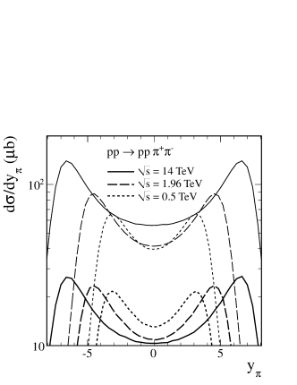
Figure 6: Differential cross section $d\sigma/dy_{\pi}$ for the $pp\to pp\pi^{+}\pi^{-}$ reaction at $\sqrt{s}=0.5,1.96,14$ TeV with $\Lambda_{off,E}^{2}=2.0$ GeV². The results without (upper lines) and with (bottom lines) absorption effects are shown.

Now we wish to compare differential distributions of pions from the $\chi_{c0}$ decay with those for the continuum pions. In the first step we calculate the two-dimensional distribution $d\sigma(y,p_{t})/dydp_{t}$, where $y$ is rapidity and $p_{t}$ is the transverse momentum of $\chi_{c}$. The decay of $\chi_{c0}\to\pi^{+}\pi^{-}$ is included then in a simple Monte Carlo program assuming isotropic decay of the scalar $\chi_{c0}$ meson in its rest frame. The kinematical variables of pions are transformed to the overall center-of-mass frame where extra cuts are imposed. Including the simple cuts we construct several differential distributions in different kinematical variables. In Fig. 7 we show distributions in pion transverse momenta. The pions from the decay are placed at slightly larger transverse momenta. This can be therefore used to get rid of the bulk of the continuum by imposing an extra cut on the pion transverse momenta.

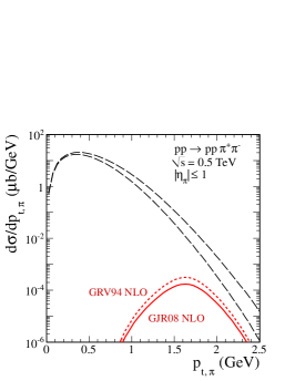
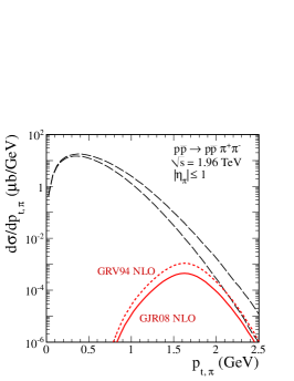
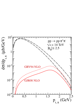
Figure 7: Differential cross section $d\sigma/dp_{t,\pi}$ at $\sqrt{s}=0.5,1.96,14$ TeV with cuts on the pion pseudorapidities. The diffractive background was obtained with the cut-off parameters $\Lambda_{off,E}^{2}$ = 1.6, 2.0 GeV² (lower and upper dashed lines, respectively). Results for the pions from the decay of the $\chi_{c0}$ meson including the $\pi^{+}\pi^{-}$ branching ratio, for GRV94 NLO (upper lines) and GJR08 NLO (bottom lines) UGDFs, are shown. The absorption effects were included in the calculations.

In Fig. 8 we show two-pion invariant mass distribution for the double-diffractive $\pi\pi$ continuum and the contribution from the decay of the $\chi_{c0}$ meson (see the peak at $M_{\pi\pi}\simeq 3.4$ GeV). In these figures the resonant $\chi_{c0}$ distribution was parameterized in the non-relativistic Breit-Wigner form:

$$\frac{d\sigma}{dM_{\pi\pi}}=\mathcal{B}(\chi_{c0}\to\pi^{+}\pi^{-})\,\sigma_{pp\to pp\chi_{c0}}\,2M_{\pi\pi}\,\frac{1}{\pi}\frac{M_{\pi\pi}\Gamma}{(M_{\pi\pi}^{2}-M^{2})^{2}+(M_{\pi\pi}\Gamma)^{2}}\,,$$ (19)

with parameters according to PDG PDG . In calculation of the $\chi_{c0}$ distribution we use GRV94 NLO and GJR08 NLO collinear gluon distributions. The cross sections for the $\chi_{c0}$ production and for the background include absorption effects. While upper row shows the cross section integrated over the full phase space at different energies, the lower row shows results including the relevant pion pseudorapidities restrictions $-1<\eta_{\pi^{+}},\eta_{\pi^{-}}<1$ (RHIC and Tevatron) and $-2.5<\eta_{\pi^{+}},\eta_{\pi^{-}}<2.5$ (LHC).

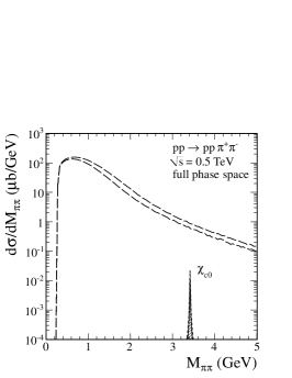
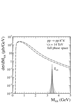
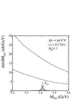
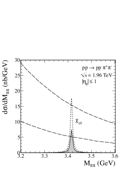
Figure 8: The $\pi^{+}\pi^{-}$ invariant mass distribution at $\sqrt{s}=0.5,1.96,14$ TeV integrated over the full phase space (upper row) and with the detector limitations in pion pseudorapidities (lower row). The dashed lines present the $\pi\pi$ continuum with the cut-off parameters $\Lambda_{off,E}^{2}$ = 1.6, 2.0 GeV² (lower and upper dashed lines, respectively). The $\chi_{c0}$ contribution is calculated with GRV94 NLO (dotted line) and GJR08 NLO (solid line) collinear gluon distributions. The absorption effects for the $\chi_{c0}$ meson and for the background were included in the calculations.

The question now is whether the situation can be improved by imposing extra cuts. In Fig. 9 we show results with additional cuts on both pion transverse momenta $|p_{t,\pi}|>1.5$ GeV. Now the signal-to-background ratio is somewhat improved especially at the Tevatron and LHC energies. Shown are only purely theoretical predictions. In reality the situation is, however, somewhat worse as both protons and, in particular, pion pairs are measured with a certain precision which leads to an extra smearing in $M_{\pi\pi}$. While the smearing is negligible for the background, it leads to a modification of the Breit-Wigner peak for the $\chi_{c0}$ meson . The results with more modern GJR UGDF are smaller by about factor of 2-3 than those for somewhat older GRV UGDF.

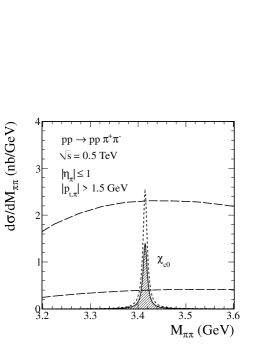
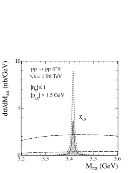
Figure 9: The $\pi^{+}\pi^{-}$ invariant mass distribution at $\sqrt{s}=0.5,1.96,14$ TeV with the relevant restrictions in the pion pseudorapidities and pion transverse momenta. The dashed lines present the $\pi\pi$ continuum with the cut-off parameters $\Lambda_{off,E}^{2}$ = 1.6, 2.0 GeV² (lower and upper dashed lines, respectively). In calculating the $\chi_{c0}$ contribution we use GRV94 NLO (dotted line) and GJR08 NLO (solid line) collinear gluon distributions. The absorption effects for the $\chi_{c0}$ meson and for the background were included. Clear $\chi_{c0}$ signal with relatively small background for the Tevatron and LHC energies can be observed when imposing extra cuts on $p_{t,\pi}$.

In Table 2 we have collected the numerical values of the cross sections (see $\sigma_{pp\to pp\chi_{c0}}$ in Eq. (19)) for exclusive $\chi_{c0}$ production for some selected UGDFs at different energies.

Table 2: Integrated cross sections in nb (with absorption corrections) for exclusive $\chi_{c0}$ production at different energies with GRV94 NLO GRV and GJR08 NLO GJR collinear gluon distributions. In this calculations we have taken the relevant limitations in the pion pseudorapidities $|\eta_{\pi}|<1$ at the RHIC and Tevatron, $|\eta_{\pi}|<2.5$ at the LHC and lower cut on both pion transverse momenta $|p_{t,\pi}|>$ 1.5 GeV.

$\sqrt{s}$	full phase space		with cuts on $\eta_{\pi}$		with cuts on $\eta_{\pi}$ and $p_{t,\pi}$
(TeV)	GRV	GJR	GRV	GJR	GRV	GJR
0.5	63.6	34.5	14.2	7.9	7.3	4.0
1.96	309.0	127.1	51.1	21.1	25.8	10.6
14	1152.3	329.7	554.1	159.1	183.7	52.2

The main experimental task is to measure the distributions in the $\chi_{c0}$ rapidity and transverse momentum. Can one recover such distributions based on the measured ones in spite of the severe cuts on pion kinematical variables? In Fig. 10 we show the two-dimensional ratio of the cross sections for the $\chi_{c0}$ meson in its rapidity and transverse momentum:

$$\mathrm{Ratio}(y,p_{t})=\frac{d\sigma^{pp\to pp\chi_{c0}(\to\pi^{+}\pi^{-})}_{\mathrm{with\;cuts}}/dydp_{t}}{d\sigma^{pp\to pp\chi_{c0}}/dydp_{t}}\,.$$ (20)

The numerator includes limitations on $\eta_{\pi}$ and $p_{t,\pi}$. These distributions provide a fairly precise evaluation of the expected acceptances when experimental cuts are imposed. The experimental data could be corrected by our two-dimensional acceptance function to recover the distributions of interest.

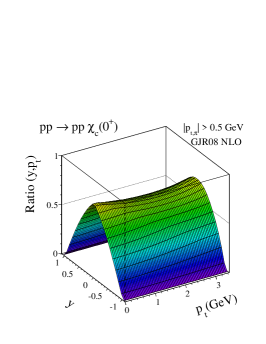
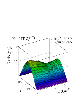
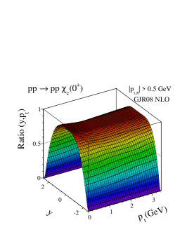
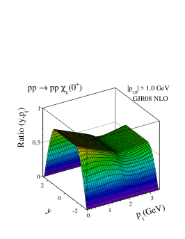
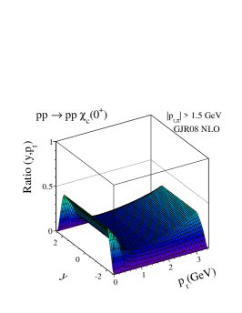
Figure 10: Ratio of the two-dimensional cross sections in $(y,p_{t})$ for the $pp\to pp\chi_{c0}$ reaction with the relevant limitations on the pion pseudorapidities and a few lower cuts on the pion transverse momenta $p_{t,\pi}$. These calculations were done with GJR08 NLO GJR UGDFs. The upper row is for the STAR detector ($|\eta_{\pi}|<1$) and the lower row for the ATLAS or CMS detectors ($|\eta_{\pi}|<2.5$).

IV Conclusions

It was realized recently that the measurement of exclusive production of $\chi_{c}$ via decay in the $J/\psi+\gamma$ channel cannot give production cross sections for different species of $\chi_{c}$. In this decay channel the contributions of $\chi_{c}$ mesons with different spins are similar and experimental resolution is not sufficient to distinguish them.

In the present paper we have analyzed a possibility to measure the exclusive production of $\chi_{c0}$ meson in the proton-(anti)proton collisions at the LHC, Tevatron and RHIC via $\chi_{c0}\to\pi^{+}\pi^{-}$ decay channel. Since the cross section for exclusive $\chi_{c0}$ production is much larger than that for $\chi_{c1}$ and $\chi_{c2}$ and the branching fraction to the $\pi\pi$ channel for $\chi_{c0}$ is larger than that for $\chi_{c2}$ ($\chi_{c1}$ does not decay into two pions) the two-pion channel should provide an useful information about the $\chi_{c0}$ exclusive production.

We have performed detailed studies of several differential distributions and demonstrated how to impose extra cuts in order to improve the signal-to-background ratio. The two-pion background was calculated in a simple model with parameters adjusted to low energy data. We have shown that relevant measurements at Tevatron and LHC are possible. At RHIC the signal-to-background ratio is much worse but measurements should be possible as well. Imposing cuts distorts the original distributions for $\chi_{c0}$ in rapidity and transverse momentum. We have demonstrated how to recover the original distributions and presented the correction functions for some typical experimental situations.

In the present paper we have concentrated on $\pi^{+}\pi^{-}$ channel only. This is mainly due to the relatively good control of the background. Measurements of other decay channels, e.g. $K^{+}K^{-}$, are possible as well and will be discussed elsewhere.

Acknowledgments

This study was partially supported by the Polish grant of MNiSW N N202 249235.

References

- (1) M.G. Albrow, T.D. Coughlin and J.R. Forshaw, Prog. Part. Nucl. Phys. 65 (2010) 149.
- (2) P. Lebiedowicz, A. Szczurek and R. Kamiński, Phys. Lett. B680 (2009) 459.
- (3) D. Alde et al. [GAMS Collaboration], Phys. Lett. 397 (1997) 350.
- (4) A. Szczurek and P. Lebiedowicz, Nucl. Phys. A826 (2009) 101.
- (5) R.S. Pasechnik, A. Szczurek and O.V. Teryaev, Phys. Rev. D78 (2008) 014007.
- (6) R.S. Pasechnik, A. Szczurek and O.V. Teryaev, Phys. Lett. B680 (2009) 62.
- (7) R.S. Pasechnik, A. Szczurek and O.V. Teryaev, Phys. Rev. D81 (2010) 034024.
- (8) L.A. Harland-Lang, V.A. Khoze, M.G. Ryskin and W.J. Stirling, Eur. Phys. J. C65 (2010) 433.
- (9) L.A. Harland-Lang, V.A. Khoze, M.G. Ryskin and W.J. Stirling, Eur. Phys. J. C71 (2011) 1545.
- (10) C. Amsler and F.E. Close, Phys. Rev. D53 (1996) 295.
- (11) T. Aaltonen et al. [CDF Collaboration], Phys. Rev. Lett. 102 (2009) 242001.
- (12) K. Nakamura et al. [Particle Data Group], J. Phys. G37 (2010) 075021.
- (13) P. Lebiedowicz and A. Szczurek, Phys. Rev. D81 (2010) 036003.
- (14) Q. He et al. [CLEO Collaboration], Phys. Rev. D78 (2008) 092004.
- (15) M. Ablikim et al. [BESIII Collaboration], Phys. Rev. D81 (2010) 052005.
- (16) M. Ablikim et al. [BESIII Collaboration], Phys. Rev. D83 (2011) 012006.
- (17) M. Ablikim et al. [BESIII Collaboration], arXiv:hep-ex/1103.2661.
-
(18)
V.A. Khoze, A.D. Martin and M.G. Ryskin, Phys. Lett. B401 (1997) 330;
V.A. Khoze, A.D. Martin and M.G. Ryskin, Eur. Phys. J. C23 (2002) 311. - (19) A.B. Kaidalov, V.A. Khoze, A.D. Martin and M.G. Ryskin, Eur. Phys. J. C33 (2004) 261.
- (20) A.B. Kaidalov, V.A. Khoze, A.D. Martin and M.G. Ryskin, Eur. Phys. J. C31 (2003) 387.
- (21) V.A. Khoze, A.D. Martin, M.G. Ryskin and W.J. Stirling, Eur. Phys. J. C35 (2004) 211.
- (22) D.V. Shirkov and I.L. Solovtsov, Phys. Rev. Lett. 79 (1997) 1209.
- (23) E.J. Eichten and C. Quigg, Phys. Rev. D52 (1995) 1726.
- (24) R. Barbieri, M. Caffo, R. Gatto and E. Remiddi, Nucl. Phys. B192 (1981) 61; W. Kwong, P.B. Mackenzie, R. Rosenfeld and J.L. Rosner, Phys. Rev. D37 (1988) 3210; M.L. Mangano and A. Patrelli, Phys. Lett. B352 (1995) 445.
- (25) A. Donnachie and P.V. Landshoff, Phys. Lett. B296 (1992) 227.
- (26) A.G. Shuvaev, K.J. Golec-Biernat, A.D. Martin and M.G. Ryskin, Phys. Rev. D60 (1999) 014015.
- (27) A.D. Martin and M.G. Ryskin, Phys. Rev. D64 (2001) 094017.
- (28) M. Glück, E. Reya and A. Vogt, Z. Phys. C67 (1995) 433.
-
(29)
M. Glück, D. Jimenez-Delgado and E. Reya, Eur. Phys. J. C53 (2008) 355;
M. Glück, D. Jimenez-Delgado, E. Reya and C. Schuck, Phys. Lett. B664 (2008) 133. - (30) V.A. Khoze, A.D. Martin and M.G. Ryskin, Eur. Phys. J. C24 (2002) 581.
- (31) J. Pumplin and F. S. Henyey, Nucl. Phys. B117 (1976) 377.
- (32) Y.I. Azimov, V.A. Khoze, E.M. Levin and M.G. Ryskin, Sov. J. Nucl. Phys. 21 (1975) 215.
- (33) A. Breakstone et al. (ABCDHW Collaboration), Z. Phys. C48 (1990) 569.
- (34) R. Waldi, K.R. Schubert and K. Winter, Z. Phys. C18 (1983) 301.
- (35) A. Breakstone et al. (ABCDHW Collaboration), Z. Phys. C42 (1989) 387.