Dynamical properties of a particle in a wave packet: scaling invariance and boundary crisis

Abstract

Some dynamical properties present in a problem concerning the acceleration of particles in a wave packet are studied. The dynamics of the model is described in terms of a two-dimensional area preserving map. We show that the phase space is mixed in the sense that there are regular and chaotic regions coexisting. We use a connection with the standard map in order to find the position of the first invariant spanning curve which borders the chaotic sea. We find that the position of the first invariant spanning curve increases as a power of the control parameter with the exponent $2/3$. The standard deviation of the kinetic energy of an ensemble of initial conditions obeys a power law as a function of time, and saturates after some crossover. Scaling formalism is used in order to characterize the chaotic region close to the transition from integrability to nonintegrability and a relationship between the power law exponents is derived. The formalism can be applied in many different systems with mixed phase space. Then, dissipation is introduced into the model and therefore the property of area preservation is broken, and consequently attractors are observed. We show that after a small change of the dissipation, the chaotic attractor as well as its basin of attraction are destroyed, thus leading the system to experience a boundary crisis. The transient after the crisis follows a power law with exponent $-2$.

1 Introduction

During the last decades many theoretical studies of area-preserving maps have intensively been done [1, 2]. One of the most studied models is the standard map proposed by B. V. Chirikov [3, 4] in 1969. The model describes the motion of the kicked rotator. The standard map can also be applied in different fields of science including accelerator physics [5], plasma physics [6] and solid state physics [7]. It has also been studied in relation to problems of quantum mechanics and quantum chaos [8, 9, 10], statistical mechanics [11] and many others.

The system we are considering in this paper is the dynamics of a particle under the action of electrostatic waves. Usually, the model is described using the formalism of discrete nonlinear maps. It is well known that the structure of the phase space in such systems depends on the combinations of both initial conditions and control parameters. Basically they are classified in three different classes: (i) integrable, (ii) ergodic and (iii) mixed. In case (i), the phase space consists of invariant tori filling the entire phase space. In case (ii), the ergodic systems have only one chaotic component, and the time evolution of a single initial condition is enough to fill the phase space [12]-[15]. Finally, the case (iii) is most common and an important property in the mixed phase space is that chaotic seas are generally surrounding Kolmogorov-Arnold-Moser (KAM) islands which are confined by a set of invariant curves. These mixed type systems are subject of intense research in classical and quantum chaos [16]-[32]. The structure of the phase space of the model we are considering is mixed and we derive analytically the location of the invariant curves. We consider a connection with the standard map close to the transition from local to global chaos and obtain an effective control parameter as well as the location of the first invariant torus bordering the chaotic sea in the phase space. In this paper we study the scaling behaviour of the model close to the transition from integrability to nonintegrability [33] in a similar way as in [34], as well as the dissipative version, and, moreover, we analyze the boundary crisis. Our main concern is the acceleration of the particle [35, 36, 37] and the saturation of the velocity [38]. An extensive work using scaling arguments was published recently in [34]. However, when the dissipative dynamics is taken into account the structure of the phase space is changed and attractors, namely, attracting fixed points and chaotic attractor, might be observed. Then, increasing the strength of the dissipation the edge of the basins of attraction of the attracting fixed points and the edge of the basin of attraction of the chaotic attractor (which corresponds to the stable and unstable manifolds of a saddle fixed point) touch each other and as a result the chaotic attractor as well as its basin of attraction is immediately destroyed. Such an event is called boundary crisis [39, 40]. After the crisis, the particle experiences a chaotic transient in the corresponding region where a chaotic attractor existed prior to the crisis. The transient is described by a power law with respect to the relative distance in the control parameter where the crisis happens.

The paper is organized as follows. In section 2 we construct the two-dimensional map that describes the dynamics of the system and discuss our numerical results. Conclusions are drawn in section 3.

2 The model and numerical results

We shall study the model of a point mass ($m$) charged ($e$) particle moving in an electric field wave packet, as introduced by G. Zaslavsky et al. [41], which in general can be written as

$$\ddot{x}=\frac{e}{m}\sum_{n=-\infty}^{\infty}E_{n}\cos(k_{n}x-\varpi_{n}t),$$ (1)

where $E_{n}$ is the amplitude of the $n$-th Fourier component of the electric field wave. They consider a wave packet with the broad spectrum, and furthermore assume $E_{n}=E_{0}$ for all $n$. Moreover, $\varpi_{n}\approx\varpi_{0}+n\Delta\varpi$ and $k_{n}\approx k_{0}+n\Delta k$. The group velocity of the wave packet is thus $v_{g}=d\varpi/dk\approx\Delta\varpi/\Delta k$. If the particle’s velocity $v=\dot{x}$ is much larger than $v_{g}$, one can use the approximation $\varpi_{n}\approx\varpi_{0}$. Using all these assumptions we get

$$\ddot{x}=\frac{e}{m}E_{0}\cos(k_{0}x-\varpi_{0}t)\sum_{n=-\infty}^{\infty}\cos(n\Delta kx),$$ (2)

and therefore using the Fourier decomposition of the periodic Dirac delta function we have

$$\ddot{x}=\frac{e}{m}LE_{0}\cos(k_{0}x-\varpi_{0}t)\sum_{n=-\infty}^{\infty}\delta(x-nL),$$ (3)

where we use $\Delta k=2\pi/L$. Between the delta kicks we have free motion of the particle and therefore the system of the two first order ordinary differential equations for $\dot{x}$ and $\dot{v}$ emerging from (3) can be formulated exactly as a discrete map. Defining $\theta=k_{0}x-\varpi_{0}t$ and $\eta=mv|v|/2$ (kinetic energy), and denoting by index $n$ their values just before the $n$-th kick, we can write this map in the following form

$$P:\left\{\begin{array}[]{ll}\eta_{n+1}=\eta_{n}+eE_{0}L\cos(\theta_{n}){}\\ \theta_{n+1}=\theta_{n}+k_{0}L~{}{\rm sign}{(\eta_{n+1})}-\varpi_{0}L\sqrt{m/2\arrowvert\eta_{n+1}\arrowvert}\end{array}\right.~{},$$ (4)

where ${\rm sign(\eta_{n+1})}=1$ if $\eta_{n+1}>0$ or $\rm sign(\eta_{n+1})=-1$ if $\eta_{n+1}<0$. However, defining $\phi=2\eta/m\varpi_{0}^{2}L^{2}$ and $\beta=\theta/2\pi-1/4$ as auxiliary variables, and introducing a dissipation parameter $\sigma$, the map $P$ can be rewritten as

$$P:\left\{\begin{array}[]{ll}\phi_{n+1}=(1-\sigma)\phi_{n}+\gamma\sin(2\pi\beta_{n}){}{}\\ \beta_{n+1}=[\beta_{n}-{1\over{2\pi|\phi_{n+1}|^{1/2}}}+\delta{\rm sign}(\phi_{n+1})]~{}~{}~{}{\rm mod(1)}\end{array}\right.~{},$$ (5)

where $\gamma=2eE_{0}/m\varpi_{0}^{2}L$, $\sigma\in[0,1]$ and $\delta=k_{0}L/2\pi$. It is important to stress that $\delta$ is just a shift of the phase and from now on we fix it as $\delta=0$ without loss of generality. Here, $\gamma$ is the control parameter which controls the transition from integrability ($\gamma=0$) to nonintegrability ($\gamma\neq 0$). As shown by Zaslavsky et al. [41] for large $\gamma>>1$ we have adiabatic picture with intermittent but largely regular behaviour. The determinant of the Jacobian matrix is ${\rm det~{}J}=1-\sigma$. So for the case of $\sigma=0$ the mapping is area preserving. Here we shall investigate some dynamical properties close to the transition from integrability to nonintegrability assuming $\gamma<<1$.

Let us first consider the conservative case where $\sigma=0$. Figure 1 (a) shows the phase space generated from Eq. (5) where the control parameter used is $\gamma=10^{-5}$. As one can see the phase space is mixed in the sense there are regular regions, invariant spanning curves (invariant tori) and KAM islands coexisting with a chaotic sea. The Lyapunov exponent is an important tool that can be used to classify orbits as chaotic or not. As discussed in [42], the Lyapunov exponents are defined as

$$\lambda_{j}=\lim_{n\rightarrow\infty}{1\over{n}}\ln|\Lambda_{j}|~{}~{},~{}~{}j=1,2~{}~{},$$ (6)

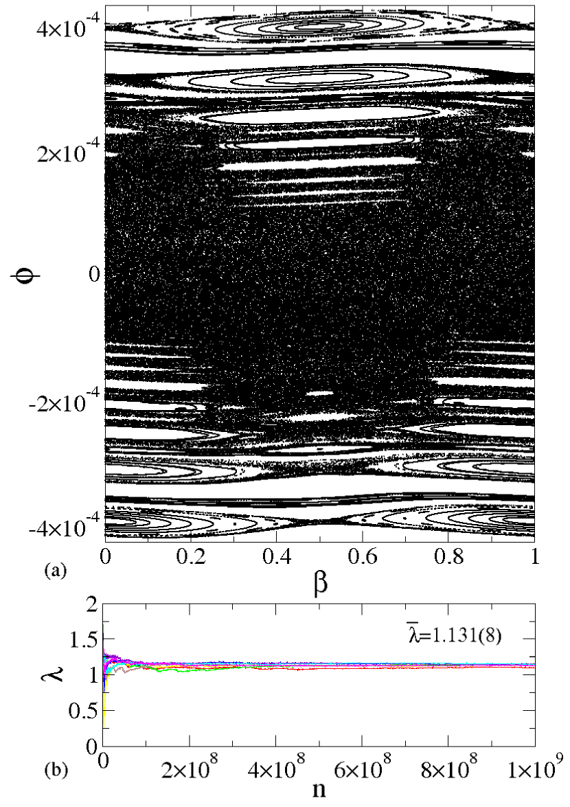
Figure 1: (Color online) (a) Phase space generated from Eq. 5 the control parameter were $\gamma=10^{-5}$; (b) Convergence of the positive Lyapunov exponent.

where $\Lambda_{j}$ are the eigenvalues of $M=\prod_{i=1}^{n}J_{i}(\beta_{i},\phi_{i})$ and $J_{i}$ is the Jacobian matrix evaluated over the orbit $(\beta_{i},\phi_{i})$. However, a direct implementation of a computational algorithm to evaluate Eq. (6) has a severe limitation to obtain $M$. Even in the limit of short $n$, the components of $M$ can assume very different orders of magnitude for chaotic orbits and periodic attractors, yielding impracticable the implementation of the algorithm. In order to avoid such problem, we note that $J$ can be written as $J=\Theta T$ where $\Theta$ is an orthogonal matrix and $T$ is a right up triangular matrix. Thus we rewrite $M$ as $M=J_{n}J_{n-1}\ldots J_{2}\Theta_{1}\Theta_{1}^{-1}J_{1}$, where $T_{1}=\Theta_{1}^{-1}J_{1}$. A product of $J_{2}\Theta_{1}$ defines a new $J_{2}^{\prime}$. In a next step, it is easy to show that $M=J_{n}J_{n-1}\ldots J_{3}\Theta_{2}\Theta_{2}^{-1}J_{2}^{\prime}T_{1}$. The same procedure can be used to obtain $T_{2}=\Theta_{2}^{-1}J_{2}^{\prime}$ and so on. Using this procedure, the problem is reduced to evaluate the diagonal elements of $T_{i}:T_{11}^{i},T_{22}^{i}$. Finally, the Lyapunov exponents are given by

$$\lambda_{j}=\lim_{n\rightarrow\infty}{1\over{n}}\sum_{i=1}^{n}\ln|T_{jj}^{i}|~{}~{},~{}~{}j=1,2~{}~{}.$$ (7)

If at least one of the $\lambda_{j}$ is positive then the system is classified as chaotic. Figure 1 (b) shows the behaviour of the positive Lyapunov exponent. We have used $10$ different initial conditions iterated in the large chaotic region up to $10^{9}$ times. The average of the positive Lyapunov exponent for our ensemble is $\bar{\lambda}=1.131(8)$, where $0.008$ corresponds to the standard deviation of the 10 samples.

The structure of the phase space of the discrete dynamical system we are dealing with and defined by the map $P$ [Eq. (5)] is illustrated in Fig. 1 (a). We can make a connection between the standard map and the map $P$ in order to find the position of the first invariant spanning curve bordering the chaotic region and also to characterize the transition from integrability to nonintegrability as it has been done in [2, 43]. The standard map was first proposed by J. B. Taylor [44] in order to study the existence of the invariants of motion in magnetic traps. Later, B. V. Chirikov [3, 4] proposed another way to obtain the map and since then it became clear that situations described by the Chirikov map occur in many physical systems. The Chirikov map is

$$C:\left\{\begin{array}[]{ll}I_{n+1}=I_{n}+K\sin\left(\Phi_{n}\right){}\\ \Phi_{n+1}=\Phi_{n}+I_{n+1}{}\end{array}\right.~{},$$ (8)

where $K$ is the control parameter (kick parameter). $K$ controls the transition from integrability, ($K=0$), to nonintegrability, ($K\neq 0$), and also controls the transition from local chaos $K<K_{c}$, where there still exists a set of invariant spanning curves separating different regions in the phase space, to global chaos, $K>K_{c}$, where all the global invariant curves are destroyed. The critical $K$ is $K_{c}=0.971635\ldots$. The connection of this result with the present model (5) is as follows. Suppose that close to the first invariant spanning curve, $\phi_{n}$ can be written as

$$\phi_{n}\cong\phi^{*}+\Delta\phi_{n}~{}$$ (9)

where $\phi^{*}$ is a typical value along the invariant spanning curve and $\Delta\phi_{n}$ is a small perturbation of $\phi$. After defining $X_{n}=2\pi\beta_{n}$, the second equation in the map (5) can be written as

$$X_{n+1}=X_{n}-{1\over{|\phi_{n+1}|^{1/2}}}~{}.$$ (10)

Using Eq. (9), we can rewrite Eq. (10) as

$$X_{n+1}=X_{n}-{1\over{|\phi^{*}|^{1/2}}}\left[1+{{\Delta\phi_{n+1}}\over{|\phi^{*}|^{1/2}}}\right]^{-1/2}~{}.$$ (11)

Expanding Eq. (11) in Taylor series and taking into account only terms of first order, we can rewrite Eq. (11) as

$$X_{n+1}=X_{n}+{1\over{|\phi^{*}|^{1/2}}}\left[1-{\Delta\phi_{n+1}\over 2|\phi^{*}|}\right]~{}.$$ (12)

Using Eq. (9), the first equation of the map (5) can also be written as

$$\phi^{*}+\Delta\phi_{n+1}=\phi^{*}+\Delta\phi_{n}+\gamma\sin(2\pi\beta_{n})~{}.$$ (13)

Multiplying both sides of Eq. (13) by ${1\over 2|\phi^{*}|}$ and adding $-{1\over|\phi^{*}|^{1/2}}$, we define

$$I_{n}=-{1\over|\phi^{*}|^{1/2}}+{{\Delta\phi_{n}\over 2|\phi^{*}|^{3/2}}}~{},$$ (14)

and re-write the map (5) as

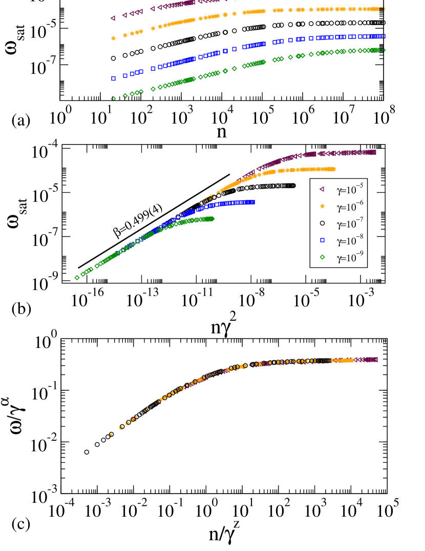
Figure 2: (Color online) (a) Behaviour of the standard deviation as function of $n$ for different values of the control parameter $\gamma$. (b) Their initial collapse after the transformation $n\gamma^{2}$. (c) Their collapse onto a single and universal plot. The different curves are coded by the symbols in the legend in the same order (top-down).

Figure 3: (Color online) (a) Plot of $\omega_{sat}$ as function of the control parameter $\gamma$. (b) Behaviour of the crossover number $n_{x}$ against $\gamma$.

$$S:\left\{\begin{array}[]{ll}I_{n+1}=I_{n}+{\gamma\over 2|\phi^{*}|^{3/2}}\sin(X_{n}){}\\ X_{n+1}=X_{n}+I_{n+1}\end{array}\right.~{},$$ (15)

Comparing the standard map [see Eq. (8)] and the map $S$, we see that there is an effective control parameter $K_{eff}$ which is given by

$$K_{eff}\cong{\gamma\over 2|\phi^{*}|^{3/2}}~{}.$$ (16)

Since the transition from local to global chaos occurs at $K_{eff}>0.971635\ldots$, the location of the first invariant spanning curve is given by

$$|\phi^{*}|\cong{\left(\gamma\over 2\times 0.971635\ldots\right)^{2/3}}~{}.$$ (17)

According to Eq. (17), the position of the first invariant spanning curve changes with exponent $2/3$ as the control parameter $\gamma$ varies. We conclude that for a given $\gamma$ a large chaotic sea is bordered by $\mid\phi\mid\leq\mid\phi^{*}\mid$. For example, for $\gamma=10^{-5}$, as in Fig. 1(a), we see indeed that $\phi^{*}\cong 2.9\times 10^{-4}$ in perfect agreement with Eq. (17). Similarly as in the standard map in such regime $I^{2}$ grows diffusively, i.e. $\overline{I^{2}}\propto n$ [45].

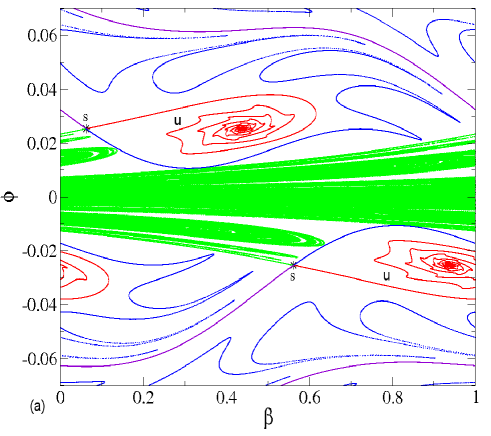
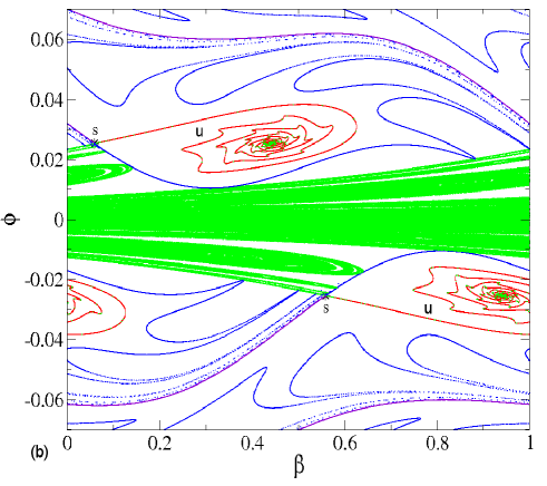
Figure 4: (Color online) Characterization of a boundary crisis. The control parameters used were $\gamma=10^{-2}$ and: (a) $\sigma=0.15$ (immediately before the crisis); (b) $\sigma=0.143$ (immediately after the crisis).

We now assume small values for the parameter $\gamma$ and study the average standard deviation of $\phi$ (kinetic energy), which is defined as

$$\omega(n,\gamma)={{1}\over{C}}\sum_{i=1}^{C}\sqrt{\overline{\phi_{i}^{2}}(n,\gamma)-{\overline{\phi_{i}}}^{2}(n,\gamma)}~{},$$ (18)

where

$$\overline{\phi}(n,\gamma)={{1}\over{n+1}}\sum_{i=0}^{n}\phi_{i}~{}.$$ (19)

We have iterated Eq. (18) up to $n=10^{8}$ for an ensemble of $C=1000$ different initial conditions. The variable $\phi_{0}$ was fixed as $\phi_{0}=10^{-2}\gamma$ and $\beta_{0}$ was uniformly distributed on $[0,1]$. Figure 2 shows the behaviour of $\omega(n,\gamma)$ as function of $n$ for five different values of the control parameter $\gamma$, as labelled in the figure. It is easy to see in Fig. 2(a) two different kinds of behaviour. For short $n$, $\omega(n,\gamma)$ grows according to a power law and suddenly it bends towards a regime of saturation for long enough values of $n$. The crossover from growth to the saturation is marked by a crossover iteration number $n_{x}$, which is very well defined by the intersection of the acceleration and saturation straight lines. It must be emphasized that different values of the parameter $\gamma$ generate different behaviors for short $n$. However, applying the transformation $n\rightarrow n\gamma^{2}$ all the curves start growing together for short $n$, as shown in Fig. 2(b). Based on the behaviour shown in Fig. 2, we can suppose the following scaling hypotheses:

1. When $n\ll{n_{x}}$, $\omega(n,\gamma)$ grows according to

   $$\omega(n\gamma^{2},\gamma)\propto({n\gamma^{2}})^{\beta}~{},$$ (20)

   where the exponent $\beta$ is the acceleration exponent;

2. For a long number of iteration, $n\gg{n_{x}}$, $\omega(n,\gamma)$ approaches a regime of saturation which is described by

   $$\omega_{sat}(n\gamma^{2},\gamma)\propto\gamma^{\alpha}~{},$$ (21)

   where the exponent $\alpha$ is the saturation exponent;

3. The crossover iteration number that marks the change from growth to the saturation is written as

   $$n_{x}\propto\gamma^{z}~{},$$ (22)

   where $z$ is the crossover exponent.

After considering these three initial suppositions, we describe $\omega(n,\gamma)$ in terms of a generalized homogeneous function of the type

$$\omega(n\gamma^{2},\gamma)=\tau\omega(\tau^{a}{n\gamma^{2}},\tau^{b}{\gamma})~{},$$ (23)

where $\tau$ is the scaling factor, $a$ and $b$ are scaling exponents that in principle must be related to $\alpha$, $\beta$ and $z$. Since $\tau$ is a scaling factor we can choose $\tau^{a}{n\gamma^{2}}=1$, or $\tau=(n\gamma^{2})^{-1/a}$. Thus, Eq. (23) is rewritten as

$$\omega(n\gamma^{2},\gamma)=({n\gamma^{2}})^{-1/a}\omega_{1}[(n\gamma^{2})^{-b/a}\gamma]~{},$$ (24)

where the function $\omega_{1}[(n\gamma^{2})^{-b/a}\gamma]=\omega[1,(n\gamma^{2})^{-b/a}\gamma]$ is assumed to be constant for $n\ll{n_{x}}$. Comparing Eqs. (20) and (24), gives us $\beta=-1/a$. Choosing now $\tau^{b}\gamma=1$, we have $\tau=\gamma^{-1/b}$ and Eq. (23) is given by

$$\omega(n\gamma^{2},\gamma)=\gamma^{-1/b}\omega_{2}(\gamma^{-a/b}n\gamma^{2})~{},$$ (25)

where $\omega_{2}(\gamma^{-a/b}n\gamma^{2})=\omega(\gamma^{-a/b}n\gamma^{2},1)$. It is also assumed as constant for $n\gg{n_{x}}$. Comparison of Eqs. (21) and (25) gives us $\alpha=-1/b$. Given the two different expressions of the saturation value $(n_{x}\gamma^{2})^{\beta}\propto\gamma^{\alpha}$, we obtain

$$n_{x}\propto\gamma^{{\alpha\over\beta}-2}~{}.$$ (26)

Thus comparing Eq. (26) and Eq. (22), the crossover exponent is $z={{\alpha/\beta}-2}$. Note that the scaling exponents are determined if the critical exponents $\beta$ and $\alpha$ were numerically obtained. The exponent $\beta$ is obtained from a power law fitting for $\omega(n\gamma^{2},\gamma)$ curves for the parameter $\gamma\in[10^{-9},10^{-5}]$ for short iteration number, $n<<n_{x}$. Thus, the average of these values gives us $\beta=0.499(4)\cong{1/2}$. Figure 3 shows the behaviour of (a) $\omega_{sat}vs.\gamma$ and (b) $n_{x}vs.\gamma$. Applying power law fitting in the figure, we obtain $\alpha=0.6736(8)\cong 2/3$ and $z=-0.657(3)$. We can also obtain the exponent $z$ evaluating $z={{\alpha/\beta}-2}$ and the previous values of both $\alpha$ and $\beta$. We found that $z=-0.651(9)$. This result indeed agrees with our numerical data. This set of critical exponents makes this transition to belongs to the same class of universality as the phase transition observed in the problem of a classical particle confined inside an infinitely deep box of potential that has an oscillating square well [46] or time varying barrier in the middle [47].

Finally, in order to confirm our initial hypotheses and, since the values of the critical exponents $\alpha$, $\beta$ and $z$ are now already known, we can use the scaling laws. Fig. 2(c) shows five different curves of $\omega$ generated from different values of the control parameter $\gamma$ overlapped onto a single universal plot.

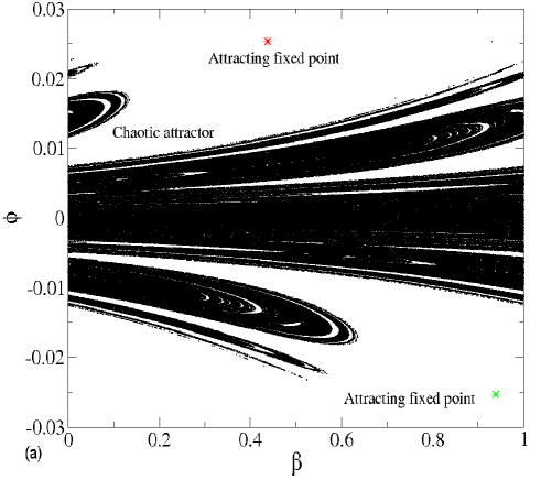
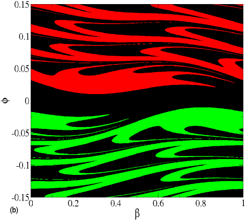
Figure 5: (Color online) (a) Attracting fixed points for $m=-1$ represented by a upperward red star, downward green star and a chaotic attractor shown in black. (b) Their corresponding basin of attraction. The control parameters used in (a) and (b) were $\gamma=10^{-2}$ and $\sigma=0.15$. The region in black is the basin of attraction of the chaotic attractor and the region in red color is the basin for the upper attracting fixed point and the region in green corresponds to the basin of attraction of the lower attracting fixed point.

Let us now present our results for the dissipative dynamics i.e. $\sigma\neq 0$. It is well known that when dissipation is considered, the mixed structure of the phase space is changed and elliptical fixed points can in principle turn into attracting fixed points (sinks) and chaotic seas might be replaced by chaotic attractors. Figure 4 shows the corresponding stable and unstable manifolds for two different saddle fixed points which are obtained by solving $\phi_{n+1}=\phi_{n}$ and $\beta_{n+1}=\beta_{n}+m$. The two solutions of these equations of map 5 are

1. $$\phi=\left[{{-1}\over{2m\pi}}\right]^{2}~{},~{}\beta^{(1)}={1\over 2\pi}{\rm\arcsin}{\left({\phi\sigma\over\gamma}\right)}~{}~{},$$ (27)

   and $\beta^{(2)}=1/2-\beta^{(1)}$, for each integer $m=\pm 1,\pm 2,\pm 3,\ldots$, and

2. $$\phi=-\left[{{-1}\over{2m\pi}}\right]^{2}~{},~{}\beta^{(1)}={{1}\over{2}}-{1\over 2\pi}{\rm\arcsin}{\left({\phi\sigma\over\gamma}\right)}~{}~{},$$ (28)

   and $\beta^{(2)}=3/2-\beta^{(1)}=1+(1/2\pi)\arcsin(\phi\sigma/\gamma)$, for each integer $m=\pm 1,\pm 2,\pm 3,\ldots$. and arcsin is evaluated on the fundamental domain $[-\pi/2,\pi/2]$ where it is uniquely defined.

For positive $\phi$ and $m=\pm 1$ in Eq. 27 we find that $\beta^{(1)}$ corresponds to the hyperbolic (saddle) fixed point, whilst $\beta^{(2)}$ corresponds to the attracting fixed point, as is illustrated in Fig. 4 (a). For the negative $\phi$ the same conclusion applies, respectively. For the whole sequence of larger $\mid m\mid\geq 2$ we have a sequence of fixed points but they can not be seen. The saddle fixed points given by Eq. (27-28) are marked by a star and are shown in the upper part of Fig. 4(a) while the Eq. (28) gives the saddle fixed point shown in Fig. 4(a) in the lower part, also marked by a star. The two branches of the unstable manifolds of each saddle are are obtained via iteration of the map $P$ with appropriate initial conditions. The upper [Eq. (27)] and lower [Eq. (28)] unstable branches are marked by $u$ and shown in red in Fig. 4. They converge to the attracting fixed points, while the downward [Eq.(27)] and upperward [Eq. (28)] branch generate the chaotic attractor and are shown in green. On the other hand, the stable manifolds consist basically in trajectories heading towards the saddle points and the construction of the stable manifolds is slightly different from those of the unstable manifolds where we have to known the inverse of the mapping $P$, which we denote by $P^{-1}$. The basic procedure is that $P^{-1}(\phi_{n+1},\beta_{n+1})=(\phi_{n},\beta_{n})$, thus the map $P^{-1}$ is given by

$$P^{-1}:\left\{\begin{array}[]{ll}\phi_{n}={\phi_{n+1}-\gamma\sin(2\pi\beta_{n})\over(1-\sigma){}}\\ \beta_{n}=\beta_{n+1}+{1\over{2\pi\mid\phi_{n+1}\mid^{1/2}}}\end{array}\right.~{}.$$ (29)

Once we have found $P^{-1}$, the stable manifolds, which corresponds to the borders between the basins of attraction for the attracting fixed points and the chaotic attractor are shown in blue and violet in Fig. 4. By reducing the value of the dissipation parameter $\sigma$ the unstable manifold of each saddle point touches simultaneously the stable manifold and as a consequence the chaotic attractor as well as its basin of attraction are immediately destroyed. Such an event is called as a boundary crisis [48, 49, 50, 51] and happens simultaneously for the manifolds arising from both Eqs. (27) and (28) as shown in Fig. 4(b) and is characterized for the first time in this model. The control parameters used in Fig. 4 were $\gamma=10^{-2}$ and: (a) $\sigma=0.15$ (immediately before the crisis); (b) $\sigma=0.143$ (immediately after the crisis).

Before the crisis and for the combination of control parameters used in Fig. 4(a) ($\gamma=10^{-2}$ and $\sigma=0.15$), there are three different attractors, namely: (i) two attracting fixed points related to $m=\pm 1$ (the central regions where the red spirals are converging to) and (ii) a chaotic attractor [see Fig. 5 (a)]. One might expect that there must be three different basins of attraction. This is indeed true as one can see in Fig. 5(b). The procedure used to obtain the basins of attraction for the chaotic and attracting fixed points consist basically in iterating a grid of initial conditions in the plane $\beta\times\phi$ and look at their asymptotic behavior. We have used a range for the initial $\beta$ as $\beta\in[0,1]$ and $\phi\in[-0.15,0.15]$. Both ranges of $\beta$ and $\phi$ were divided in $1000$ parts each, leading to a total of $10^{6}$ different initial conditions and for the values of the control parameters that we have considered, each combination of $(\beta,\phi)$ was iterated up to $10^{5}$ times. After the crisis, the time evolution of an initial condition in the corresponding region of the chaotic attractor before the crisis leads the orbit to make an incursion towards the region of the, now, chaotic transient until being captured by one of the two sinks. The structure of the two basins of attraction belonging to the two attracting fixed points is very complex and it is shown in Fig. 6, so that it is difficult to decide which initial condition will go to which of the two attractors, as there are some obviously some regions in the phase spcae where both basins of attraction are dense.

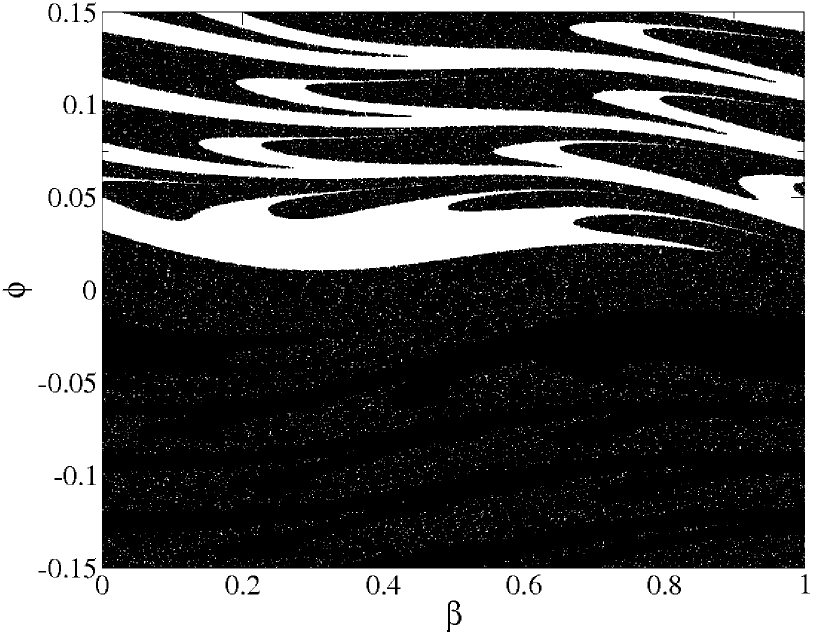
Figure 6: (Color online) Basins of attraction of the two sinks observed in the phase after the boundary crisis. The interwoven structure is evident. The control parameters used were $\gamma=10^{-2}$ and $\sigma=0.143$.

We may therefore argue that an initial condition chosen in the region of the phase space that produced a chaotic dynamics before the crisis, now gives rise to a chaotic transient. We denote as transient the corresponding number of iterations that the orbit typically spends until it finds the appropriate route to one of the attracting fixed points. The transient is described by a power law of the type

$$n_{t}\propto\mu^{\zeta}~{},$$ (30)

where $\mu=\sigma-\sigma_{c}$ with $\sigma_{c}<\sigma$. For a fixed $\gamma=0.01$, our numerical simulations lead to the critical value of $\sigma_{c}=0.143056\ldots$. Figure 7

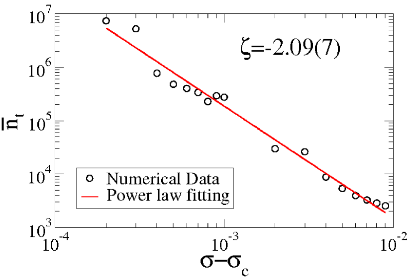
Figure 7: (Color online) Plot of $n_{t}~{}{\rm vs.}\mu$ for a fixed $\gamma=0.01$. A power law fitting gives $\zeta=-2.09(7)$.

shows the behaviour of the average transient plotted as a function of $\mu$ considering a fixed $\gamma=0.01$. A power law fitting gives the exponent $\zeta=-2.09(7)$. The procedure used to simulate the transient consists in evolving in time an ensemble of $B=5\times 10^{3}$ different initial conditions randomly chosen along the region of the chaotic attractor as observed just before the crisis, and calculated the time $n_{t}^{i}$, where $i$ is a member of the ensemble, that the particle spends until reaches one of the two attracting fixed points. The average transient is calculated as

$$\bar{n_{t}}={{1}\over{B}}\sum_{i=1}^{B}n_{t}^{i}~{},$$ (31)

where $i$ specifies an orbit of the ensemble. The exponent $\zeta=-2.09(7)$ has, within an uncertainty error, the same value as the exponent obtained for the boundary crisis observed in a dissipative Fermi-Ulam model [49]. The Fermi-Ulam model consists of a classical particle that is confined to bounce between two rigid walls. One of them is fixed and the other one is periodically time-varying. Despite the remarkable difference of the two models (the main difference being the power of the term in the denominator of the two mappings, which is $1$ in the Fermi-Ulam model and $1/2$ in our model), the chaotic transient after the boundary crisis marking the converging to the attracting fixed points follows the same rule in both models and is given by the same exponent $\cong-2$.

3 Conclusions

We have studied the problem of a charged particle in the electric field of a wave packet. We have confirmed through analytical arguments that close to the invariant spanning curves the dynamics of our model can be described by the standard map. Such approach allows us to find the position of the first invariant spanning curve (chaos border) as a function of the control parameter $\gamma$. Once we have found that the position of the first invariant torus changes as a power of the control parameter $\gamma$ with the exponent $2/3$, we have studied the behaviour of the chaotic sea close to the transition from integrability to nonintegrability (small values of the control parameter $\gamma$) using scaling arguments. We have shown that there exists an analytical relationship between the critical exponents, namely, acceleration exponent, saturation exponent and crossover exponent. Our scaling hypotheses have been confirmed by the perfect collapse of all curves onto a single universal plot. Finally, for the dissipative dynamics we have found the expressions for the saddle fixed points and constructed the corresponding unstable and stable manifolds. We have shown that increasing the dissipation, the unstable manifold touches the stable manifold and the chaotic attractor as well as its basin of attraction are completely destroyed. We have shown that such a destruction is caused by a boundary crisis. Finally the transient marking the approach to the sink is characterized by a power law with exponent $\cong-2$.

References

- [1] G. M. Zaslavsky, Hamiltonian Chaos and Fractional Dynamics (Oxford, 2006).
- [2] A. J. Lichtenberg, M. A. Lieberman Regular and Chaotic Dynamics Appl. Math. Sci. Vol 38 (Springer Verlag, New York, 1992).
- [3] B. V. Chirikov, Research concerning the theory of nonlinear resonance and stochasticity, Preprint N 267, Institute of Nuclear Physics, Novosibirsk (1969).
- [4] B. V. Chirikov, A universal instability of many-dimensional oscillator systems, Physics Reports 52 (1979), p. 263.
- [5] F. M. Izraelev, Nearly linear mappings and their applications, Physica D 1 (1980),p. 243.
- [6] T. H. Stix, Current penetration and plasma disruption, Phys. Rev. Lett. 36 (1976), p. 10.
- [7] H. L. Cycon, R. Froese, W. Kirsch, B. Simon Schrödinger Operators (Berlin, Springer, 1987).
- [8] H.-J. Stöckmann, Quantum Chaos: An Introduction (Cambridge University, Cambridge, England, 1999)
- [9] F. Haake, Quantum Signatures of Chaos (New York, Springer-Verlag, 2001).
- [10] G. Casati, I. Guarneri, J. Ford, F. Vivaldi, Search for randomness in the kicked quantum rotator, Phys. Rev. A 34 (1986), p. 1413.
- [11] S. Aubry, The twist map, the extended Frenkel-Kontorova model and the devil’s staircase, Physica D 7 (1983), p. 240.
- [12] L. A. Bunimovich, On the Ergodic Properties of Nowhere Dispersing Billiards, Commun. Math. Phys. 65 (1979), p. 295.
- [13] E. D. Leonel, A. L. P. Livorati, Describing Fermi acceleration with a scaling approach: bouncer model revisited, Physica A 387 (2008), p. 1155.
- [14] A. L. P. Livorati, D. G. Ladeira, E. D. Leonel, Scaling investigation of Fermi acceleration on a dissipative bouncer model, Physical Review E 78 (2008), p. 056205.
- [15] D. F. M. Oliveira, J. Vollmer, E. D. Leonel, Fermi acceleration and suppression of Fermi acceleration in a time-dependent Lorentz gas, Physica D 240 (2011), p. 389.
- [16] M. V. Berry, Regularity and chaos in classical mechanics, illustrated by three deformations of a circular billiard. Eur. J. Phys. 2 (1981) p. 91.
- [17] M. Robnik, Classical dynamics of a family of billiards with analytic boundaries, J. Phys. A: Math. Gen. 16 (1983), p. 3971.
- [18] M. V. Berry, M. Robnik, Semiclassical level spacings when regular and chaotic orbits coexist, J. Phys. A 17 (1984), p. 2413.
- [19] M. Robnik, M. V. Berry Classical billiards in magnetic fields, J. Phys. A: Math. Gen. (1985) 18, p. 1361.
- [20] T. Prosen, M. Robnik, Energy level statistics in the transition region between integrability and chaos, J. Phys. A 26 (1993), p. 2371.
- [21] T. Prosen, M. Robnik, Survey of the eigenfunctions of a billiard system between integrability and chaos, J. Phys. A 26 (1993), p. 5365.
- [22] T. Prosen, M. Robnik, Numerical demonstration of the Berry-Robnik level spacing distribution, J.Phys.A 27 (1994), p. L459.
- [23] T. Prosen, M. Robnik, Semiclassical energy level statistics in the transition region between integrability and chaos: Transition from Brody-like to Berry-Robnik behaviour, J.Phys.A 27 (1994), p. 8059.
- [24] M. Robnik, Topics in quantum chaos of generic systems, Nonlinear Phenomena in Complex Systems 1 (1998), p. 1.
- [25] T. Prosen, M. Robnik, Intermediate statistics in the regime of mixed classical dynamics, J. Phys. A: Math. Gen. 32 (1999), p.1863.
- [26] S. O. Kamphorst, S. P. de Carvalho, Bounded gain of energy on the breathing circle billiard, Nonlinearity 12 (1999), p. 1363.
- [27] R. Markarian, S. O. Kamphorst, S. P. de Carvalho, Chaotic properties of the elliptical stadium, Commun. Math. Phys. 174 (1996), p. 661.
- [28] G. Veble, M. Robnik, J. Liu, Study of regular and irregular states in generic systems, J. Phys. A 32 (1999), p. 6423.
- [29] G. Veble, U. Kuhl, M. Robnik, H.-J. Stöckmann, J. Liu, M. Barth, Experimental Study of Generic Billiards with Microwave Resonators, Prog. Theor. Phys. Suppl. 139 (2000), p. 283.
- [30] V. Lopac, I. Mrkonjić, D. Radić, Chaotic dynamics and orbit stability in the parabolic oval billiard, Phys. Rev. E 66 (2001), p. 036202.
- [31] E. D. Leonel, P.V. E. McClintock, A hybrid Fermi-Ulam-bouncer model, J. Phys. A 38 (2005), p. 823.
- [32] V. Lopac, I. Mrkonjić, N. Pavin, D. Radić, Chaotic dynamics of the elliptical stadium billiard in the full parameter space, Physica D 217 (2006), p. 88.
- [33] E. D. Leonel, P. V. E. McClintock, J. k. L. Silva, The Fermi-Ulam Accelerator Model Under Scaling Analysis, Phys. Rev. Lett. 93 (2004), p. 014101.
- [34] J. A. de Oliveira, R. A. Bizão, E. D. Leonel, Finding critical exponents for two-dimensional Hamiltonian maps, Phys. Rev. E, 81 (2010), p. 046212.
- [35] F. Lenz, F. K. Diakonos, P. Schmelcher, Tunable Fermi Acceleration in the Driven Elliptical Billiard, Phys. Rev. Lett. 100 (2008), p. 014103.
- [36] E. D. Leonel, D.F.M. Oliveira, A. Loskutov, Fermi acceleration and scaling properties of a time dependent oval billiard, Chaos 19 (2009), p. 033142.
- [37] F. Lenz, C. Petri, F. K. Diakonos, P. Schmelcher, Phase-space composition of driven elliptical billiards and its impact on Fermi acceleration, Phys. Rev. E 82 (2010), p. 016206.
- [38] D. F. M. Oliveira, E. D. Leonel, Suppressing Fermi acceleration in a two-dimensional non-integrable time-dependent oval-shaped billiard with inelastic collisions, Physica A 389 (2010), p. 1009.
- [39] C. Grebogi, E. Ott, J. A. Yorke, Chaotic attractors in crisis, Phys. Rev. Lett. 48 (1982), p. 1507.
- [40] C. Grebogi, E. Ott, J. A. Yorke, Crises, sudden changes in chaotic attractors, and transient chaos, Physica D 7 (1983), p. 181.
- [41] G. M. Zaslavsky, R. Z. Sagdeev, D. A. Usikov, A. A. Chernikov, Weak Chaos and Quasi-Regular Patterns (Cambridge Nonlinear Science Series) Cambridge University Press 1991).
- [42] J.-P. Eckmann, D. Ruelle, Ergodic Theory of Chaos and Strange Attractors, Rev. Mod. Phys. 57 (1985), p. 617.
- [43] E. D. Leonel, J. K. L. Silva, S. O. Kamphorst, On the dynamical properties of a Fermi accelerator model, Physica A 331 (2004), p. 435.
- [44] J. B. Taylor, Colham Lab. Prog. Report CLM-PR-12 (1969).
- [45] D.F.M. Oliveira, M. Robnik, E.D. Leonel, Statistical properties of a dissipative kicked system: critical exponents and scaling invariance, submitted (2011).
- [46] E. D. Leonel, P. V. E. McClintock. Scaling properties for a classical particle in a time-dependent potential well, Chaos 15, (2005) p. 33701.
- [47] E. D. Leonel, P. V. E. McClintock, Chaotic properties of a time-modulated barrier, Phys. Rev. E 70, (2004), p. 016214.
- [48] E. D. Leonel, P. V. E. McClintock, A crisis in the dissipative Fermi accelerator mode, J. Phys. A 38 (2005), p. L425.
- [49] E. D. Leonel, R. Egydio de Carvalho, A family of crisis in a dissipative Fermi accelerator model, Phys. Lett. A 364 (2007), p. 475.
- [50] D. F. M. Oliveira, E. D. Leonel, Boundary crisis and suppression of Fermi acceleration in a dissipative two-dimensional non-integrable time-dependent billiard, Phys. Lett. A 374 (2010), p. 3016.
- [51] D. F. M. Oliveira, E. D. Leonel, M. Robnik, to be submitted (2011).