Extended X-ray emission in the vicinity of the microquasar LS 5039: pulsar wind nebula?

Abstract

LS 5039 is a high-mass binary with a period of 4 days, containing a compact object and an O star, one of the few high-mass binaries detected in $\gamma$-rays. Our Chandra ACIS observation of LS 5039 provided a high-significance ($\approx 10\sigma$) detection of extended emission clearly visible for up to 1′ from the point source. The spectrum of this emission can be described by an absorbed power-law model with photon index $\Gamma=1.9\pm 0.3$, somewhat softer than the point source spectrum $\Gamma=1.44\pm 0.07$, with the same absorption, $N_{H}=(6.4\pm 0.6)\times 10^{21}$ cm^-2. The observed 0.5–8 keV flux of the extended emission is $\simeq 8.8\times 10^{-14}$ erg s^-1cm^-2, or 5% of the point source flux; the latter is a factor of $\sim 2$ lower than the lowest flux detected so far. Fainter extended emission with comparable flux and a softer ($\Gamma\approx 3$) spectrum is detected at even greater radii (up to 2′). Two possible interpretations of the extended emission are a dust scattering halo and a synchrotron nebula powered by energetic particles escaping the binary. We discuss both of these scenarios and favor the nebula interpretation, although some dust contribution is possible. We have also found transient sources located within a narrow stripe south of LS 5039. We discuss the likelihood of these sources to be related to LS 5039.

1 Introduction

In a high-mass X-ray binary (HMXB), a compact object, which can be a black hole (BH) or a neutron star (NS), accretes some portion of the wind from a high-mass ($M>5M_{\odot}$) non-degenerate companion star. Some HMXBs are called ‘micro-quasars’ ($\mu$QSOs) when resolved, collimated radio features are observed, which are interpreted as relativistic jets.

There has been renewed interest in $\mu$QSOs since the detection of parsec-scale X-ray jets (Corbel, 2007) and variable $\gamma$-ray emission (Abdo et al., 2009b). The nature of the high-energy emission for two micro-quasars, LS 5039 and LS I +61 303, has been much debated, e.g., the emission could truly be generated in a $\mu$QSO jet (Khangulyan et al., 2008), or possibly it could be generated by the interaction of a young pulsar wind with the wind of the companion (Leahy, 2004; Dhawan et al., 2006; Dubus, 2006).

LS 5039 was first identified as an HMXB by Motch et al. (1997) based on the positional coincidence of an X-ray source with an O7V star ($V=11.5$), projected near the Galactic bulge ($l=16\fdg 8816$, $b=-1\fdg 2892$). Using optical and infra-red spectroscopy, Clark et al. (2001) found the companion star to be type O6.5V(f), variable in the IR but not in the optical. McSwain et al. (2001) measured line radial velocities and found binary period $P_{\rm orb}=4.1$ d and substantial eccentricity $e=0.4$. Using detailed time-resolved spectroscopy and atmospheric modeling of the companion, Casares et al. (2005) refined the binary parameters ($P_{\rm orb}=3.906$ d, $e=0.35$) and concluded that the system must harbor a high-mass compact object, probably a BH, for an inferred distance of $2.5\pm 0.1$ kpc. The conclusion was, however, later disputed by Dubus (2006) who argued that the NS option still cannot be dismissed. Using high-precision, long time base-line photometry from the MOST satellite and ground-based spectroscopy, Sarty et al. (2011) further refined the orbital characteristics, preferring a slightly lower eccentricity $e=0.24\pm 0.08$ and component masses 26$M_{\odot}$ for the O-star and 1.7$M_{\odot}$ for the compact object. Thus, the nature of the compact object in LS 5039 remains unknown.

An unresolved, non-thermal, variable radio source was fist detected by Marti et al. (1998). Using the high angular resolution of VLBA, the source was resolved, and ‘jets’ observed by Paredes et al. (2000); the source was therefore classified as a $\mu$QSO. Ribó et al. (2002) measured the system proper motion ($\approx$12 mas yr^-1, using radio and optical astrometry) and, based on its high tangential velocity, called the system ‘runaway’, i.e., with enough velocity to leave the Galactic disk. The proper motion vector can be traced back to the supernova remnant (SNR) G16.8$-$1.1. Subsequent radio observations by Ribó et al. (2008) showed that the resolved emission of LS 5039 varies in intensity, and that the position angle of the elongated features changes.

LS 5039 has been extensively observed in X-rays, mainly to study its variability and spectrum. The X-ray emission is modulated at the orbital period. The light-curve produced from X-ray data taken in 1999-2007 was found to be remarkably stable (Kishishita et al., 2009), although some aperiodic variability has been reported earlier with RXTE (Reig et al., 2003; Ribó et al., 1999).

Both LS 5039 and LS I +61 303 have been detected at higher energies. LS 5039 has been detected with HESS (Aharonian et al., 2006), INTEGRAL (Hoffmann et al., 2009) and Fermi (Abdo et al., 2009a), with a spectrum similar to $\gamma$-ray pulsars. The high-energy light curves show modulations at the orbital period, peaking at superior conjunction (see Bosch-Ramon & Khangulyan 2009 for a review).

In this paper we report the results of a 38 ks imaging observation of LS 5039 with Chandra. In Section 2, we describe our data and reduction procedures, as well as several archival data sets. In Section 3 we analyze the spectra of both the point source and the extended emission, calculate radial profiles, and examine the extended morphology. We also describe the properties of a number of transient sources that appear in the field. In Section 4 we discuss our findings and their implications. We conclude with a brief summary in Section 5. We also include Appendix A, in which we calculate the X-ray contribution due to dust scattering in the direction of LS 5039.

2 Observations and data analysis

Table 1 lists the X-ray observations considered in this work, including five archival observations (from XMM-Newton and Chandra) and our latest Chandra observation.

Table 1: Log of observations

Date	ObsID	Telescope/	Off-axis	Exposure
		instrument	angle (′)	time (ks)
2004-07-09	4600	Chandra/ACIS	12	11.0
2004-07-11	5341	Chandra/ACIS	12	18.0
2005-04-13	6259	Chandra/ACIS	0	5.0
2005-09-22	0202950201	XMM/EPIC	0	15.8
2005-09-24	0202950301	XMM/EPIC	0	10.4
2009-10-30	10696	Chandra/ACIS	3	37.8

Note. — Exposure times are live (i.e., corrected for GTI filtering and dead-time).

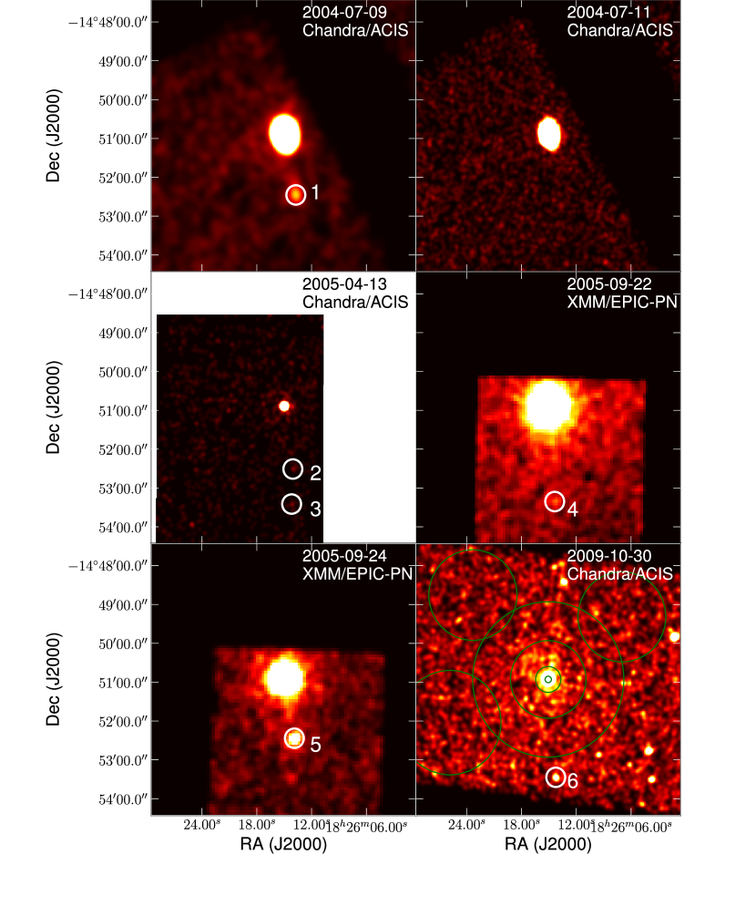
Figure 1: Images of the field of LS 5039. All images are 7′$\times$7′, in the 0.59–6.8 keV energy band for Chandra, 1–7 keV for XMM-Newton. In the bottom-right panel we mark the source and background extraction regions used in our spectral analysis (green circles; see §3.2). White numbered circles show the faint field point sources discussed in §3.3.

2.1 New Chandra observation

LS 5039 was observed with the Advanced CCD Imaging Spectrometer (ACIS) on board Chandra on 2009 October 30 (ObsID 10696). Our observation spanned orbital phases $\phi=0.064$–0.184 (using the ephemeris of Casares et al. 2005, where $\phi=0$ corresponds to periastron). The target was observed for 38.55 ks in timed exposure mode using “very faint” telemetry format. To minimize pile-up effects, we used a custom 750 pixel wide sub-array and turned off all the ACIS chips except I3. The frame time in this configuration is 2.24104 s (2.2 s exposure time and 0.04104 s image transfer time). The Y-offset was $-2\farcm 8$, placing the source 3$\farcm$03 off axis. This resulted in a broader PSF, further helping to mitigate pile-up. There were no significant background flares during the observation. The useful scientific exposure time (live-time) was 37.84 ks.

The data were reduced and analyzed with the Chandra Interactive Analysis Observations (CIAO) package (ver. 4.2), using CALDB 4.2.0. To produce images of the pulsar and its vicinity at subpixel resolution, we removed the pipeline pixel randomization and applied the subpixel resolution tool to split-pixel events in the image (Mori et al., 2001).

The image produced from this data is shown as the bottom-right panel in Figure 1.

2.2 Archival observations

We downloaded archival observations of LS 5039, three by Chandra and two by XMM-Newton, see Table 1. In the case of the Chandra data, we used the standard Level 2 calibrated science event files. We used the energy range 0.59–6.8 keV, which is the optimal range for viewing the extended emission (see below), and show the resultant images in Figure 1. Although taken with the same instrument, the data sets span a range of exposure times and off-axis distances.

In the case of the XMM-Newton data, we made use of only the EPIC-PN data, from the standard pipeline in the XMM-SAS calibration package. These data were filtered in the energy range 1–7 keV, and the resultant images are also shown in Figure 1.

We performed no further processing on any of these archival data, and use them only for comparison purposes while looking for transient sources (§3.3).

In addition to the six observations discussed in this paper, there were two observations by Chandra and two by XMM-Newton. The Chandra data were taken in continuous-clocking mode, and so are not useful for analysis either of extended emission or faint field sources because of the much higher background. For the XMM observations, the spacecraft orientation was such that the locations of faint field sources shown in Figure 1 were not imaged, and again the PSF is too broad and the background too high to see extended emission. We consider neither observation further, except to note the point source flux measured by Chandra, below.

3 Results

From the images in Figure 1, it appears that LS 5039 is a bright unresolved point source with extended emission around it; the extended emission is seen most clearly in the latest Chandra observation (bottom right panel). We split our results into three sections: the spectrum of the bright point source, which is essentially unaffected by faint extended emission, the properties of the extended emission, which includes some contribution by the bright source’s PSF, and a description of the transient sources in the field.

3.1 Point source

From the Chandra ACIS data of 2009 October 30, we extracted the spectrum of the point-like source corresponding to LS 5039, centered at coordinates ${\rm R.A.}=276\fdg 56278$, ${\rm decl.}=-14\fdg 84871$ (J2000), using the CIAO task psextract. We picked background regions far from the source, and as free of point sources as possible, yet large enough (total area 51,100 arcsec²) that the background spectrum be well-determined. The extraction regions are shown on Figure 1.

We fitted an absorbed power-law (PL) model to the spectrum, extracted from the $r=5\arcsec$ aperture, using the Sherpa package. We grouped the counts in 25-count bins and fitted in the energy range 0.5–8 keV (4602 counts in total, of which 3.8 counts belong to the background; source count rate $0.122\pm 0.002$ counts s^-1). The observed energy flux is $F_{\rm 0.5-8\,keV}=(1.92\pm 0.03)\times 10^{-12}$ erg cm^-2 s^-1. The fitting parameters are given in Table 2, and the fluxed count-rate spectrum is shown in Figure 2.

The inferred extinction-corrected flux for the 1–10 keV range is 2.6$\times 10^{-12}$ erg cm^-2 s^-1. Although the phase interval of our observation corresponds to the minimum of the previously observed orbital variability, this is a factor of two lower than any flux that has been noted in the past (e.g., the long-term study by Kishishita et al. 2009; Takahashi et al. 2009). For two Chandra observations a few months before, 2009 July 31 (observation ID 10053) and August 6 (observation ID 10932; PI Nanda Rea), with orbital phases $\phi=$0.81-0.95 and 0.35-0.43, we found fluxes 8.7$\times 10^{-12}$ erg cm^-2 s^-1 and 7.7$\times 10^{-12}$ erg cm^-2 s^-1, respectively, close to the values previously measured at these phases.

With a count rate of 0.27 counts per frame, the pile-up fraction would be 10% if the target were on-axis (estimated using Chandra PIMMS). As the source was $\approx 3^{\prime}$ off-axis in our observation, the actual pile-up fraction is about 4%, as we estimated with the aid of MARX simulations (see below).

Table 2: Power-law spectral fits

Region	Radius range (″)	$N_{H}$ (cm-2)	$\Gamma$	$A$	$\chi^{2}/{\rm dof}$	$F_{\rm 0.5-8\,keV}^{\rm unabs}$
Point source	0-5	$6.4(6)\times 10^{21}$	1.44(7)	35.1(3)	139.3/176	25.4(2)
Extended	20-60	6.4$\times 10^{21}$	1.9(7)	2.9(7)	47/40	1.4(3)
Extended	60-120	6.4$\times 10^{21}$	3.1(5)	8(2)	70/103	2.4(6)

Note. — Fits were performed in the 0.5–8 keV energy range. Numbers in parentheses are $1\sigma$ uncertainties on the last digit. Confidence contours are shown in Figure 3.

Our best-fit photon index, $\Gamma=1.44\pm 0.07$, is only marginally consistent with those previously measured at the same orbital phase, $\Gamma=$1.55-1.6 (Kishishita et al., 2009).

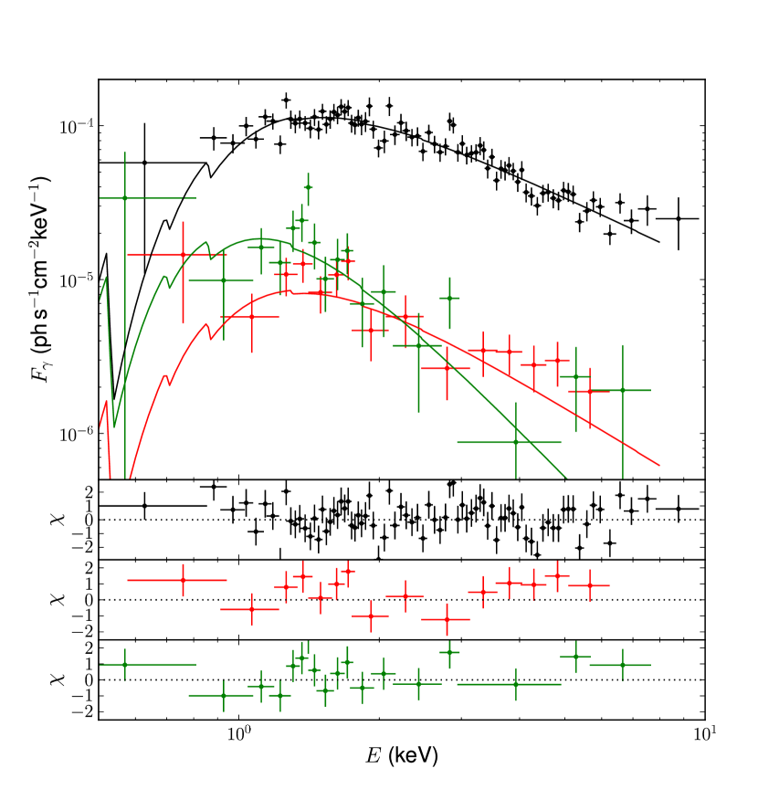
Figure 2: Fluxed spectrum of LS 5039 (black) and the extended emission extracted from 20″–60″ (red) and 60″–120″ (green) annuli around LS 5039. Best-fit absorbed power-law models are over-plotted as solid lines, and residuals, $\chi=({\rm data-model)/uncertainty}$ are shown in the lower three panels. The best-fit model and fitting parameters were estimated using standard forward-fitting (i.e., by fitting the count-rate spectrum).

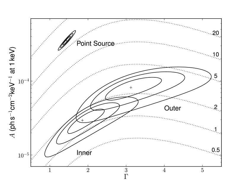
Figure 3: Confidence contours at one-, two- and three-sigma, for the PL fit to the spectra. The fits to the annular spectra have $N_{H}$ fixed to the value obtained for the point source. Lines of constant unabsorbed flux in the 0.5–8 keV band are shown with dotted lines, and labeled in units of $10^{-13}$ erg s^-1cm^-2.

3.2 Extended emission

We used Chandra Ray Tracer (ChaRT) and MARX software to simulate the PSF for the given spectrum and location on the detector. In order to reduce the Poissonian noise, we made a simulated event file for 200 ks exposure, filtered the same way as for real data, and then scaled by the exposure times. We used ChaRT with the input spectrum derived from our spectral fit to the central point source and MARX Version 4.4 with parameters ACIS_Exposure_Time=2.2 (to account for the non-standard sub-array mode) and DitherBlur=0.27 (a measure of the aspect reconstruction accuracy and pixelization by the detector, typically near 0$\farcs$3 for ACIS). All other parameters were left at their default values.

The simulated PSF is shown in Figure 4. We calculated the signal-to-noise ratio (S/N) of the extended emission near the point source, and found the optimum energy range 0.59–6.8 keV. In the radii range 20″–60″, we find 745 counts, of which expect 378 from the background and 81 from the PSF wings, giving $286\pm 29$ source counts, a detection significance of $9.9\sigma$. In the radii range 60″–120″, there are 1766 counts, of which 1278 should be background and 32 from the PSF wings, giving $456\pm 51$ source counts, a detection significance of about $8.9\sigma$.

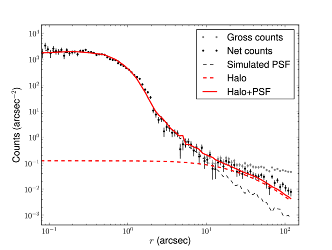
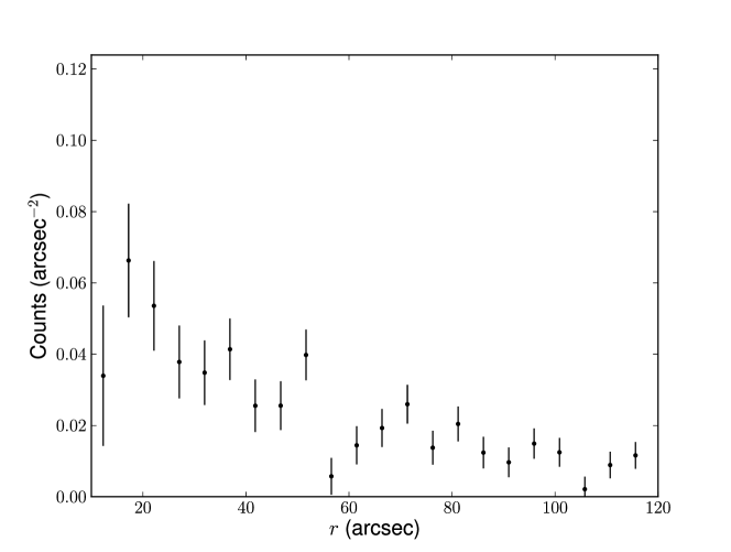
Figure 4: Top: Radial intensity plot around the point source, for the total (gross), background subtracted (net), simulated PSF count intensities and dust scattering halo model in the energy range 0.59–6.8 keV. Bottom: The difference between the net and PSF curves, i.e., the excess emission around the point source.

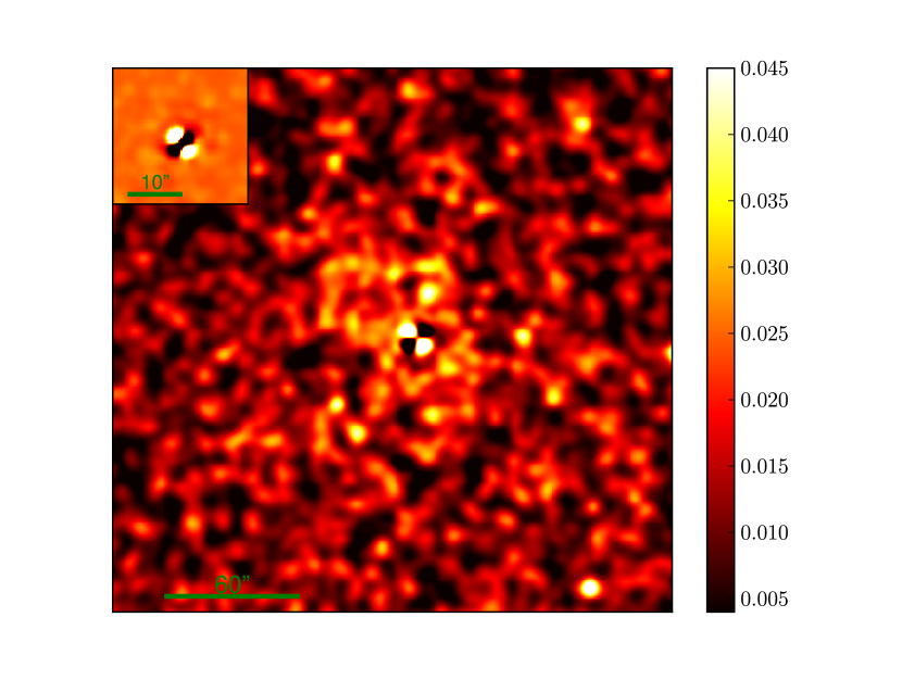
Figure 5: 256″$\times$256″ image of the vicinity of LS 5039 after subtraction of the simulated PSF. The color-bar scale is counts per 0$\farcs$49$\times$0$\farcs$49 pixel. The image has been smoothed by a Gaussian kernel with $r=3\arcsec$. The inset shows the central 27″$\times$27″ section, where binning was 0$\farcs$25, and smoothing width $r=0\farcs 5$. It better demonstrates the residual structure around the point source, likely caused by imperfections in the PSF model.

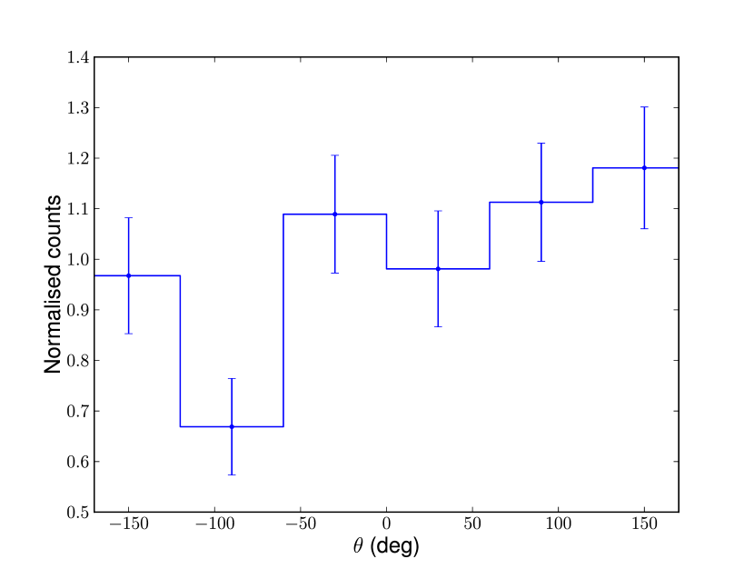
Figure 6: Histogram of total counts in the $r=20\arcsec$–60″annulus and optimal energy range (0.59–6.8 keV), as a function of azimuthal angle about the point source, with zero angle west and increasing towards the north.

To analyze the spectrum of the extended emission, we extracted counts from the two annular regions, $r=20\arcsec$–60″and $r=1\arcmin$–2′, using the CIAO task specextract. The background regions were the same as for the point source above (see Figure 1). The spectra were once more grouped to at least 25 counts per bin, and fitted with an absorbed PL model in the energy range 0.5–8 keV. The column density was kept fixed at the best-fit value obtained from the fit to the point source spectrum ($N_{H}=6.4\times 10^{21}$ cm^-2). For the inner annulus, there is considerable contamination from the PSF wings, which may have a different spectrum from the point source because of the energy dependence of the the PSF. To account for this, we fit the counts extracted from the simulated PSF events in the same annulus, and then include this as an additional frozen component ($\Gamma=0.59$, $N=3.83\times 10^{-7}$pn s^-1cm^-2keV^-1 is 1 keV) when fitting the extended emission. The results of the fits are shown in Table 2, while the corresponding fluxed spectra and confidence contours are shown in Figures 2 and 3, respectively. The observed energy flux was $F_{\rm 0.5-8\,keV}=(8.8\pm 1.9)\times 10^{-14}$ erg cm^-2s^-1 (inner) and $(7.5\pm 1.9)\times 10^{-14}$ erg cm^-2s^-1 (outer). Using the ‘optimal’ energy range as defined above gives very similar fit parameters. We find that the inner annulus spectrum is only slightly softer than the point source, while the outer annulus is significantly softer.

To better see the morphology of the extended emission, we subtracted the model PSF from the original image. The relative positions of the simulated and observed sources were adjusted to minimize the residuals. The result is shown in Figure 5. Some extended structure is apparent, such as wisps to the north and east. With the relatively low S/N it is hard to say more, but, interestingly, similar structure is visible in the short on-axis Chandra observation of 2005 April 13 (Figure 1). To quantify any anisotropy, we considered the distribution of the extended emission over azimuthal angles about the point source. Figure 6 shows a net histogram of background- and PSF-subtracted counts for the inner annulus. The distribution appears to be non-uniform, with $\chi^{2}=15.9$ for 5 degrees of freedom for a constant value (null hypothesis probability of 0.7%).

The difference between the simulated and point source images shows residuals up to $r=3\arcsec$, although the two agree well in the radial plot (Figure 4). This suggests some imperfections in the PSF model on small scales.

3.3 Transient field sources

A number of small brightness enhancements are apparent in the images in Figure 1. We have labeled the significant ones with white markers. They are all consistent with being point-like, although with the small numbers of counts, this is not very restrictive.

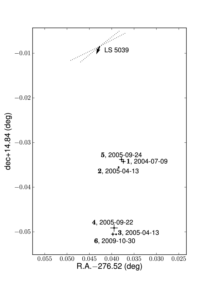
Figure 7: Detected sources in the field of LS 5039. We show LS 5039’s proper motion vector (1000 times yearly value measured by Ribó et al. 2002, black arrow) and the position angles of radio elongation at two different epochs (dashed lines; Ribó et al. 2008). The object numbers (bold) refer to the white labels in Figure 1.

Table 3: Fluxes of transient field source fluxes

Date	Sources	Flux
		North	South
2004-07-09	1	$3.6\pm 0.8$	$<$4.4
2004-07-11		$<$0.8	$<1.4$
2005-04-13	2,3	$2.4\pm 1.1$	$2.3\pm 1.7$
2005-09-22	4	$<$0.7	$1.3\pm 0.3$
2005-09-24	5	$3.1\pm 0.5$	$<$2.0
2009-10-30	6	$<$0.47	$1.6\pm 0.4$

The numbered sources in Figure 1 are projected onto the same sky coordinates in Figure 7. They appear to lie within a narrow stripe almost due south from LS 5039 in two clumps or clusters. All the sources have rather hard spectra (mean energies 2–4 keV). Notably, the source that was bright on 2004 July 9 (Source 1) had completely disappeared two days later (even though the latter observation had a longer exposure time, and would have detected it); similarly Source 5 appeared on a similar time-scale. We cannot exclude that sources 1 and 5 are the same object, see below. The fluxes of these sources are given in Table 3.

We show zoomed-in views of the locations of the field sources detected during observations of LS 5039. In Figure 8 the positions are plotted, after bore-sight correction, along with sources from the 2MASS catalog (Skrutskie et al., 2006). The nearest 2MASS sources, which have positions consistent with (some of) the field sources, are listed in Table 4 their infra-red magnitudes. Where possible, we also include optical magnitudes.

Sources 2 and 3 are only marginal detections. If they are not real sources, or if they are unrelated to the rest of the sources detected, then it is likely that sources 1 and 5 are a single flaring source possibly associated with 2MASS source C. Likewise, sources 4 and 6 could be a single persistent source, perhaps associated with 2MASS source A.

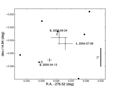
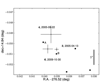
Figure 8: Close-up of the locations of field sources shown in Figure 7, northern group (left) and southern group (right). Also shown are sources from the 2MASS catalog (squares). The nearest stars are labeled by letters, and their photometric data and positions are given in Table 4. The coordinates shown here are after the application of a bore-sight correction. Scale bars are 5″ in length.

Table 4: Photometry and positions of 2MASS sources near faint X-ray sources

Label	2MASS ID	$J$	$H$	$K_{\rm S}$	Other	R.A. (°)	decl (°)
					photometry
A	18261441-1453235	14.40	12.62	11.91		276.560075	$-$14.889871
B	18261416-1453275	13.68	12.64	12.22		276.559035	$-$14.890979
C	18261389-1452239	14.40	$>$13.50	$>$13.28	$B=16.64,V=16.20$	276.557879	$-$14.873326
D	18261419-1452324	12.50	11.03	10.46	$R=19.4$	276.559134	$-$14.875684

Note. —  Labels refer to the those shown in Figure 8. 2MASS photometric uncertainties are 0.04-0.06 mag.

4 Discussion and conclusions

Our analysis has revealed a highly significant extended emission discernible up to $\simeq 2^{\prime}$ from LS 5039 (limited by the FOV boundaries). This emission could be either due to the dust scattering of X-rays emitted by the unresolved source or it could be emission from relativistic particles escaping from the vicinity of LS 5039. Below we discuss both options. In addition, we observed at least two faint unresolved sources. These could be field stars, background highly-absorbed CVs or quiescent XRBs (or even AGNs seen through the Galactic plane), but they might in principle be manifestations of a collimated outflow from LS 5039.

The flux of the point source LS 5039 was a factor of $\sim$2 lower than expected for its orbital phase, despite previously appearing to have a stable orbital light-curve (Kishishita et al., 2009). Previous studies did suggest larger variability (Reig et al., 2003; Ribó et al., 1999), but the use of different instrumentation (particularly RXTE) made the variability hard to verify. A decrease in flux could perhaps be explained by a change in accretion state (if the compact source is a BH) but even for pulsar emission, it can be explained by changes in the wind properties of the companion O-star which also manifest themselves via the variability of H_α emission (Reig et al., 2003).

4.1 Dust scattering halo

Scattering of X-rays emitted by the unresolved source off the dust lying along the line of sight produces extended emission known as a dust scattering halo (e.g., Predehl & Schmitt 1995). The halo brightness scales linearly with the intervening dust column, which is usually assumed to be proportional to the hydrogen column density, $N_{H}$, measured from X-ray spectra, i.e., scattering optical depth at 1 keV is $\tau_{{\rm s,1keV}}\simeq S(N_{H}/10^{22}~{}{\rm cm}^{-2})$, where the proportionality constant $S$ can only be determined empirically and depends on properties of the intervening dust which may differ for different objects. For instance, Predehl & Schmitt (1995) found a mean $S\simeq 0.5$ from their sample of X-ray halos, which corresponds $\tau_{{\rm s,1keV}}\simeq 0.24$ for LS 5039 where $N_{H}=6.4\times 10^{21}$ cm^-2 (Table 2). An even better correlation for $\tau_{{\rm s}}$ was obtained with the optical extinction towards the object, $\tau_{{\rm s,1keV}}=0.056A_{V}$ (see Appendix A), which gives $\tau_{{\rm s,1keV}}=0.22$ (for $A_{V}=3.9$; Ribó et al. 2002), in good agreement with the previous estimate. The relatively low value of $\tau_{{\rm s,1keV}}$ allows us to neglect the contributions of multiple scatterings for $E\gtrsim 1$ keV.

We have calculated the halo profile in the single-scattering approximation by folding the spectral intensity of a halo (see e.g., Mathis & Lee 1991, also Appendix A) with the detector response in the 0.5–8 keV energy range. We find that, for instance, for the parameters $\Theta=360\arcsec$ and $S=1$, and the dust distribution function $f(x)$ defined in Appendix A, the dust halo model overall describes the observed radial profile (see Fig. 4). Although some deviations are noticeable, they might be attributed to the imperfect choice of the above parameters (we did not perform rigorous fitting) or to the inaccuracy of the Draine (2003) model or the Rayleigh-Gans (RG) approximation to the scattering cross section at low energies ($\lesssim 2$ keV).

The dust distribution function $f(x)$ used to calculate the halo model (see Equation (A8) and Figure 4) assumes a lack of absorption/scattering in the immediate vicinity of the source. Such dust distribution is consistent with the lack of evidence of significant intrinsic absorption in the LS 5039 binary. The upper limit on the intrinsic column density is as low as $2.6\times 10^{21}$ cm^-2 (Bosch-Ramon et al., 2007; Takahashi et al., 2009), while the total absorbing column density measured from X-ray spectra changes by $\lesssim 10\%$ (Takahashi et al., 2009) with binary phase. Low intrinsic absorption would be expected if most of X-rays are emitted far from the donor star, where its wind is sufficiently rarefied (e.g. Szostek & Dubus 2011).

We should also point out that, in addition to the dust distribution profile, the dust scattering model we use has two free parameters ($S$ and $\Theta$) which can attain values within rather broad ranges, depending on the actual properties of the dust grains. Therefore, the mere fact that the model qualitatively fits the observed brightness distribution does not guarantee that the extended emission is a dust halo. In fact, the observed azimuthal asymmetry and the hard spectrum of the inner extended emission would be difficult to explain by a dust halo. Significant spectral softening is expected from halo models. Specifically, for the dust model used, the spatially integrated (between $r=20^{\prime\prime}$ and $60^{\prime\prime}$) spectrum is expected to have $\Gamma_{\rm halo}\simeq\Gamma_{\rm point}+2\simeq 3.5$, because the scattering cross-section $\sigma_{s}(E)\propto E^{-2}$ (see Appendix A). Instead, we find a significantly harder spectrum, $\Gamma\approx 1.9$. On the other hand, the outer extended emission is indeed much softer and more symmetric, hence could have some contribution from a halo.

4.2 Extended nebula of LS 5039

The nature of the compact object (BH or NS) in LS 5039 remains subject of a debate. LS 5039  (and LS I +61 303) are quite different in their temporal and spectral properties from other $\mu$QSOs and HMXBs, which show transitions between different states and large variations in luminosity. These two systems are also, to date, the only $\mu$QSOs whose VHE emission has been firmly detected. The X-ray light curve of LS 5039, which shows remarkable long-term stability (Kishishita et al., 2009; Takahashi et al., 2009; Hoffmann et al., 2009), and peculiar, variable radio morphology (Ribó et al., 2008) argue against the accretion scenario.

If, despite the lack of the usual manifestations of accretion, the compact object in LS 5039 is a BH accreting in an unusual regime (Casares et al., 2005), it may still be possible that it produces relativistic particles, e.g., via the Blandford-Znajek process (Blandford & Znajek, 1977) or in an MHD jet. In this case, an extended nebula could still be formed. For the case of a black hole, the majority of high-energy emission is expected to be produced in a jet-type axial outflow (e.g., Paredes et al. 2006). The possible observational manifestations of such outflows and a discussion of their energetics is discussed by Russell & Fender (2010) and their extended emission by Heinz et al. (2008). The relativistic electrons responsible for the $\gamma$-ray emission in the inner jet will cool with distance. Flow speeds are typically close to $c$ (Yadav, 2006), and so X-ray emission can be expected out to appreciable distances from the black hole, e.g., the plasma clumps seen by Corbel et al. (2002) up to $\sim 30$″ from $\mu$QSO XTE J1550-564. Furthermore, the spin axis of the black hole may precess, and so the orientation of the outflow change with time, as with SS 334 (Blundell et al., 2007) and thus fill an extended volume with energetic emission, rather than the more typical collimated outflows. Such large-angle precession may be hard to explain, however, possibly requiring a third massive component to the system.

A possible alternative interpretation of the high-energy emission from LS 5039  is a pulsar wind nebula (PWN) powered by a young, energetic pulsar. In this scenario, modeling of the intra-binary shock suggests that the O-star wind dominates dynamically over the pulsar wind, which makes the shocked wind flow away from the head of the intra-binary bow-shock and along the bow-shock surface which is curved away from the O-star (see e.g., Figures 1 and 2 in Szostek & Dubus 2011). If the opening angle of the bow-shock is small, it would resemble a cometary tail rotating around the O-star together with the pulsar and pointing in the direction of the O-star wind (cf.  variable radio morphology of LS I +61 303 resolved with VLBI; Dhawan et al. 2006; see also the discussion in Pavlov et al. 2011a). Emission from the innermost regions of the bow-shock may be responsible for the unresolved, bright X-ray source whose surface brightness varies with the orbital phase owing to Doppler boosting (Dubus et al., 2010). Since the tail is rotating, it winds itself into a tight spiral, which at larger distances from the pulsar and with limited angular resolution would appear as disk-like emission concentrated toward the orbital plane. Moreover, it seems reasonable to assume that, in this disk, the pulsar wind becomes well mixed with the dynamically dominant companion wind and that both are advected away at the O-star wind terminal speed, $v_{\infty}$, at distances $r\gg a$ (where $a$ is the orbital separation). Adopting $v_{\infty}=2400$ km s^-1 (McSwain et al., 2004), we can estimate the time it takes for the wind to reach the angular distance $\alpha$ as t${}_{\rm dyn}\simeq 300(\alpha/1\arcmin)(v_{\infty}/2400~{}{\rm km~{}s}^{-1})^{-1}$ yr.

The likely emission mechanism in this case would be synchrotron radiation (see below), implying the cooling time $t_{\rm syn}\sim 300(E/5~{}{\rm keV})^{-1/2}(B/10~{}\mu{\rm G})^{-3/2}$ yrs. Requiring $t_{\rm syn}\gtrsim t_{\rm dyn}$ places an upper limit on the average magnetic field in the extended emission region,
$B\lesssim 10(E/5~{}{\rm keV})^{-1/3}(v_{\infty}/2400~{}{\rm km~{}s}^{-1})^{2/3}(\alpha/1^{\prime})^{-2/3}$ $\mu$G, where $E$ is the observed energy of synchrotron photons emitted by relativistic electron with Lorentz factor
$\gamma\sim 3\times 10^{8}(E/5~{}{\rm keV})^{1/2}(B/10\,\mu{\rm G})^{-1/2}$. Since the upper limit on $B$ is not much higher than the value of the magnetic field in the ISM, it is likely that the actual magnetic field is on the order of 10 $\mu$G, and hence the electron Lorentz factor should be of the same order as those in ordinary PWNe around isolated pulsars. On the other hand, the inferred $\gamma$ is close to the maximum possible Lorentz factor estimated by Dubus (2006) by requiring the electron gyro-radius to be less than the size of the acceleration region, assumed to be on the order of the standoff distance for the intra-binary shock. Moreover, Dubus (2006) concluded that electrons will not attain $\gamma\gtrsim 10^{8}$ because of the strong synchrotron radiative losses in the innermost regions. Additional acceleration outside the intra-binary shock (e.g., via magnetic reconnection in the spiral-like tail) may provide a way to circumvent this limitation. Alternatively, $\gamma$ could be somewhat lower if the magnetic field is higher than estimated above, which is possible if the bulk flow speed if somewhat higher than the terminal O-star wind speed. Indeed, up to a certain distance, the fast pulsar wind could provide some re-acceleration to the O-star wind until both components become well mixed. However, the detailed modeling of this complex interaction is beyond the scope of this paper. The observed softening of the extended emission with the distance from the point source could be attributed to synchrotron cooling which can be substantial at $\alpha\gtrsim 1^{\prime}$ if $B\sim 10$ $\mu$G or somewhat larger.

Inverse Compton (IC) and adiabatic expansion cooling compete with synchrotron cooling and can even dominate, depending on the distance from the particle acceleration region (the intra-binary shock). Although at the distances of interest here, the O-star radiation energy density, $\epsilon_{\rm rad}=3.8\times 10^{-10}(\alpha/1^{\prime})^{-2}$ erg cm^-3, would exceed the magnetic field energy density, $\epsilon_{\rm B}=4.0\times 10^{-12}(B/10~{}\mu{\rm G})^{2}$ erg cm^-3, the IC cooling of $\gamma\gtrsim 6\times 10^{4}$ electrons occurs in the Klein-Nishina regime and is hence inefficient in comparison with the competing processes (see Blumenthal & Gould 1970). Indeed, the relevant IC cooling time, $\tau_{\rm IC}\sim 20(E/5~{}{\rm keV})^{1/2}(B/10\,\mu{\rm G})^{-1/2}(\alpha/1^{\prime})^{2}$ Myr, on the O-star light will be much larger than the corresponding synchrotron cooling time of electrons emitting $E=5$ keV photons in $B=10$ $\mu$G. On the other hand, the same electrons will also cool via IC upscattering of CMB photons, and this process will dominate over the IC scattering on O-star light at the distances of interest. IC scattering off the CMB proceeds in Thompson regime with characteristic cooling time $\tau_{\rm IC,CMB}\simeq 7(E/5~{}{\rm keV})^{-1/2}(B/10\,\mu{\rm G})^{1/2}$ kyr, which is still larger than the corresponding $\tau_{\rm syn}$ (see above). Finally, there is also cooling due to adiabatic expansion, which, in 2D geometry, has a characteristic cooling timescale comparable to dynamic timescale (see, e.g. Eqn. (28) in Dubus 2006).

Zdziarski et al. (2010) suggested that the X-ray emission from the compact (unresolved) PWN in LS I +61 303 could be produced via IC scattering of stellar photons by the pulsar wind electrons with $\gamma\sim 20$. The synchrotron emission by the same electrons is expected to be in the radio, while the GeV emission could be interpreted as IC up-scattering of stellar light by more energetic photons with $\gamma$ up to $2\times 10^{4}$. If the electron SED in LS 5039  extends down to such low $\gamma$, these processes may contribute significantly at sufficiently small distances from the binary. As the low-energy electrons should remain unaffected either by IC or synchrotron cooling on any plausible dynamical timescales, one would expect to see radio synchrotron emission on much larger angular scales than it has been reported. Deep radio observations, sensitive to extended structures on arcsecond–arcminute scales, can provide a useful diagnostics in this case.

From modeling of absorption and occultation, Szostek & Dubus (2011) estimated the plausible range of $\dot{E}=(0.1$–$38)\times 10^{36}$ erg s^-1 for the alleged pulsar in LS 5039. The observed unabsorbed luminosity $L_{\rm 0.5-8\,keV}=1\times 10^{32}d_{2.5}^{2}$ erg s^-1 implies the radiative efficiency range $3\times 10^{-6}$–$10^{-3}$, which well matches the range for resolved PWNe around subsonically-moving isolated Vela-like pulsars ($10^{-5}$–$10^{-3}$; Figure 7 in Kargaltsev et al. 2007; Kargaltsev & Pavlov 2008). If LS 5039 is indeed associated with SNR G16.8$-$1.1, it has a kinematic age of 40–150 kyr, i.e., a factor of a few older than the Vela-like pulsars listed in Table 2 of Kargaltsev et al. (2007). This would favor lower values of efficiency from the range given above, and, correspondingly, lower O-star mass loss rates from the range discussed in Szostek & Dubus (2011).

If the extended emission is due to the pulsar wind, there can be non-variable TeV emission associated with the extended wind-filled region, even larger than that resolved in X-rays, resembling relic PWNe around isolated pulsars (see e.g., Kargaltsev & Pavlov 2010). Indeed, Aharonian et al. (2006) reported orbital modulation of the LS 5039 TeV flux peaking near inferior conjunction phase but also reported a second component with a different spectrum seen near the light curve minimum. While the harder emission at the peak of the light curve is likely to come from the innermost region of the binary, the soft spectrum of the second component is akin to those of TeV PWNe (see Kargaltsev & Pavlov 2010 and references therein) and could be attributed to the extended PWN. Therefore, further high-sensitivity, high-resolution observations in TeV are certainly warranted.

4.3 Transient sources in the field

We have found several (at least two, see §3.3) transient X-ray sources, all of which are distributed within a very narrow strip south of LS 5039. Taken together, the positions of these sources at different epochs are inconsistent with a constant velocity or uniformly decelerated motion of a single source (see Figures 1 and 7). Therefore, they cannot represent the propagation of a single clump of plasma ejected by LS 5039. The sources could be unrelated flaring objects (e.g., heavily absorbed background CVs in the central region of the Galaxy) or, alternatively, all could be flare-ups in an outflow largely invisible in X-rays, in which case they don’t have to be causally connected. Although relativistically outflowing plasma clumps have been seen before in $\mu$QSOs, their variability at such large distances from the central source has never been seen as dramatic as would appear to be the case here (e.g., Blundell et al. 2007; Corbel et al. 2002). The direction of this outflow would be different from that of the two radio jets seen on milli-arcsecond scales, but the latter were seen to change orientation by 12°$\pm 3\arcdeg$ (Ribó et al., 2008).

We have searched for other variable sources within the XMM-Newton EPIC-PN FOVs (the smallest FOVs among the observations; see Figure 1) and did not find any other variable sources. Further monitoring of LS 5039 with Chandra or XMM-Newton is needed to draw any definitive conclusions on the nature of the transient sources we discovered. Confirming ejecta clumps would favor accretion/ejection scenario over the pulsar wind one.

4.4 Comparison with LS I +61 303 and B1259$-$63

Among known HMXBs, the one that resembles LS 5039 the most is LS I +61 303. In both systems, the donor stars are massive early type stars (O and Be stars with masses 23$M_{\odot}$ and 12$M_{\odot}$, in LS 5039 and LS I +61 303, respectively). Both exhibit very similar X-ray properties (including fluxes, spectral slopes, $N_{H}$; e.g., Rea et al. 2010) and are located at similar distances. Recently, both systems were detected in GeV and TeV, where they also share many common properties such as similar VHE spectra and light curves (Hill et al. 2010, and references therein). Among the differences are a factor of 7 larger orbital period ($P_{\rm orb}=26.5$ days) and a factor of 2 larger eccentricity ($e=0.72$) of the LS I +61 303 orbit. Also, LS I +61 303 appears to be more variable in X-rays, sometimes showing short flares (Torres et al., 2010). This could be due to non-uniformity of the companion wind which is believed to be concentrated in a rather thin disk in the equatorial plane (Sierpowska-Bartosik & Torres, 2009). The compact object interacts with this dense wind only during a relatively short phase interval while it crosses the disk (Sierpowska-Bartosik & Torres, 2009). The wind of the O-star in LS 5039 is believed to be much more isotropic. Analyzing a 49 ks Chandra ACIS observation of LS I +61 303, Paredes et al. (2007) found faint ($58\pm 18$ counts) asymmetric excess emission extending $\approx 12\arcsec$ from the point source. This emission was not confirmed in the subsequent longer (96 ks) Chandra ACIS observation, but that observation used Continuous Clocking mode with much higher background and only one spatial dimension, greatly complicating the analysis (Rea et al., 2010). Finding a much fainter extended emission around LS I +61 303  while having the point source X-ray properties very similar to those of the LS 5039 point source, supports the conclusion that most of the extended emission in LS 5039  is not a dust scattering halo, if the gas-to-dust ratios and dust grain properties are similar for these two systems. If the extended emission around the two sources were both dust halos, then, with a similar dust grain size distribution, the dust-to-gas ratio would need to be a factor of 10 larger towards LS 5039 in order to explain the brighter halo. The dust-to-gas ratio is known to have large scatter along different sight-lines, however (see Appendix A).

If the extended emission around LS 5039 is due to particles supplied by the pulsar wind, one could speculate that this emission should be fainter in LS I +61 303 because there the pulsar spends most of the time outside the dense companion wind, and hence the pulsar wind is not as efficiently confined and decelerated as in LS 5039. This means that in LS I +61 303 most of the pulsar wind is leaving the binary with large bulk velocity, which should result in much larger but fainter X-ray nebula, undetectable in existing data.

Another object of possibly similar nature is B1259$-$63, a HMXB with a much wider orbit ($P_{\rm orb}=3.4$ yr), high eccentricity ($e=0.87$) and a known pulsar ($P=48$ ms, $\dot{E}=8.3\times 10^{35}$ erg s^-1), where Pavlov et al. (2011a) found evidence of extended emission. In that case, the emission is confined to $r<15\arcsec$. This shows that a pulsar system is indeed capable of creating extra-binary extended X-ray emission, and therefore that such a scenario may be valid for the case of LS 5039, although in this case on a much larger spatial scale.

5 Summary

We have discovered asymmetric emission around LS 5039, extending up to 2′ from the point source. Although it is possible that some of this emission is due to a dust scattering halo, most of it is likely produced by energetic particles emanating from LS 5039. Although large-scale energetic jets have been observed emanating from $\mu$QSOs, there is a lack of an obvious mechanism to fill a large extended volume with X-ray-emitting particles; the pulsar scenario for the compact object appears to be preferable. If the wind nebula interpretation of the extended emission is true, one would expect to find an even larger radio and/or GeV/TeV nebula, in sensitive enough observations. We find transient sources in the field in a narrow stripe south of LS 5039 whose nature is unclear.

Appendix A Dust halo model

Dust halos, often seen around bright point-like X-ray objects, are formed by scattering of source X-ray photons on dust grains. Here we will only discuss the case of dust optically thin with respect to the photon scattering, $\tau_{\rm scat}\lesssim 1$, and consider only azimuthally symmetric halos (which implies that the dust distribution across the line of sight (LOS) is uniform within the interval of angles $\theta$ at which we see the halo). In this case the spectral halo intensity (ph cm^-2 s^-1 keV^-1 arcmin^-2) is given by the equation

$$I_{\rm halo}(\theta,E)=F(E)N_{H}\int_{0}^{1}dx\,\frac{f(x)}{x^{2}}\,\frac{d\sigma_{s}(E,\theta_{s})}{d\Omega_{s}}\,,$$ (A1)

where $F(E)$ is the point source spectral flux (photons cm^-2 s^-1 keV^-1), $x=(D-d)/D$ is the dimensionless distance from the X-ray source to the scatterer ($D$ and $d$ are the distances from the observer to the source and the scatterer, respectively), $\theta_{s}\simeq\theta/x$ (for small angles) is the scattering angle, $f(x)$ is the dimensionless dust density distribution along the LOS ($\int_{0}^{1}f(x)\,dx=1$), and $d\sigma_{s}(E,\theta_{s})/d\Omega_{s}$ is the differential scattering cross section per one hydrogen atom, averaged over the dust grain distribution over sizes and other grain properties (see, e.g., Mathis & Lee 1991). Here we assume that the source spectrum $F(E)$ does not vary: strong variability in the source can change the appearance of the halo in a complicated way, as time-lag depends upon radial distance from the source.

To understand the halo properties from simple analytical expressions, we will use the Rayleigh-Gans (RG) approximation, in which the total scattering cross section $\propto E^{-2}$; this approximation works better for higher energies, $E\gtrsim 0.5$–2 keV, depending on the dust model. For some dust models, the averaged differential cross section in the RG can be approximated as (Draine 2003)

$$\frac{d\sigma_{s}(E,\theta_{s})}{d\Omega_{s}}\approx\frac{\sigma_{s}(E)}{\pi\theta_{s,50}^{2}}\,\frac{1}{(1+\theta_{s}^{2}/\theta_{s,50}^{2})^{2}}\,,$$ (A2)

where

$$\theta_{s,50}\approx\frac{\Theta}{E}\quad{\rm and}\quad\sigma_{s}(E)\approx\frac{S}{E^{2}}\,10^{-22}\,{\rm cm}^{2}$$ (A3)

are the median scattering angle and the total cross section, respectively; $E$ is the energy in keV. The constant $\Theta$ in first eq. (A3) depends on the dust model; Draine (2003) derived $\Theta=360^{\prime\prime}$ from the dust model of Weingartner & Draine (2001), while Bocchino et al. (2010) found $\Theta=7.4^{\prime}$ for the model of Smith & Dwek (1998).

It follows from the second eq. (A3) that the scattering optical depth is

$$\tau_{\rm scat}(E)\approx SN_{H,22}E^{-2}.$$ (A4)

The factor $S$ in the second eq. (A3) is a constant of the order of 1; e.g., $S\approx 1.3$ from Figure 6 of Draine (2003), while Predehl & Schmitt (1995) found a mean value $S\approx 0.49$ for a number of halos observed with ROSAT (but the scatter was very large), while Mathis & Lee (1991) discuss models with $S=0.903$, 1.09, and 0.47 (see their Table 1). Costantini (2004; PhD thesis) estimated $\tau_{\rm sca}(1\,{\rm keV})$ for a number of halo sources observed with Chandra; the values of $S$ derived from her results show a very strong scatter, $S$ from 0.018 to 2.26. The scatter itself may be natural, as the dust properties may be different for different sources.

It should be noted that the correlation of $\tau_{\rm sca}(1\,{\rm keV})$ with visual extinction $A_{V}$:

$$\tau_{\rm scat}(1\,\,{\rm keV})=(0.056\pm 0.01)A_{V}$$ (A5)

(Predehl & Schmitt, 1995) is better than that with $N_{H}$, but $A_{V}$ is rarely known for the objects of interest.

Substituting (A2) and (A3) in (A1), we obtain the spectral intensity profile

$$I_{\rm halo}(\theta,E)=F(E)N_{H,22}\frac{S}{\pi\Theta^{2}}\int_{0}^{1}\frac{f(x)}{x^{2}}\,\left[1+\left(\frac{\theta E}{x\Theta}\right)^{2}\right]^{-2}dx\,.$$ (A6)

For comparison with the point source + halo profile observed in the energy range $E_{1}<E<E_{2}$, the sum of the spectral intensities should be convolved with the detector response, with allowance for the image spread caused by the telescope and the detector. We have checked that the energy redistribution in the detector only slightly affects the broadband radial profile for a smooth incident spectrum. Therefore, assuming the observable halo size to be much larger than the PSF width, we obtain

$$I_{\rm obs}(\theta)=\int_{E_{1}}^{E_{2}}dEA_{\rm eff}(E)\,F(E)\,\left\{\psi(\theta,E)+N_{H,22}\frac{S}{\pi\Theta^{2}}\int_{0}^{1}dx\frac{f(x)}{x^{2}}\left[1+\left(\frac{\theta E}{x\Theta}\right)^{2}\right]^{-2}\right\},$$ (A7)

where $A_{\rm eff}(E)$ is the detector’s effective area, and $\psi(\theta,E)$ is the normalized PSF, which can be taken from a simulation (e.g., with MARX for Chandra images). The first term in Equation (A7) corresponds to the point source, while the second term describes the halo.

The above equation can be integrated for a given set of halo parameters, and compared directly with the data. In particular, for the dust halo model shown in Figure 4 we picked $\Theta=360\arcsec$, $S=1$, and the dust distribution function

$$f(x)=\begin{cases}0&\textrm{$x<x_{1}$,}\\ (x_{2}-x_{1})^{-1}&\textrm{$x_{1}\leq x\leq x_{2}$,}\\ 0&\textrm{$x>x_{2}$},\end{cases}$$ (A8)

for $x_{1}=0.1$, $x_{2}=0.6$. According to (A6), this distribution corresponds to the following profile of spectral intensity

$$I_{\rm halo}(\theta,E)=\frac{F(E)N_{H,22}S}{2\pi\theta^{2}E^{2}(y_{2}-y_{1})}\left[\arctan\frac{y_{2}-y_{1}}{1+y_{1}y_{2}}-\frac{(y_{2}-y_{1})(1-y_{1}y_{2})}{(1+y_{1}^{2})(1+y_{2}^{2})}\right]\,,$$ (A9)

where $y_{i}=x_{i}\Theta/(\theta E)$. For small, intermediate, and large $\theta$, Equation (A9) turns into

$$I_{\rm halo}(\theta,E)\simeq\frac{F(E)N_{H,22}S}{\pi\Theta^{2}}\begin{cases}(x_{1}x_{2})^{-1}&\theta\ll x_{1}\Theta/E,\\ (\pi/4x_{2})(\Theta/\theta E)&x_{1}\Theta/E\ll\theta\ll x_{2}\Theta/E,\\ (1/3)(\Theta/\theta E)^{4}(x_{1}^{2}+x_{1}x_{2}+x_{2}^{2})&\theta\gg x_{2}\Theta/E,\end{cases}$$ (A10)

where the approximation for the intermediate $\theta$ implies $x_{2}\gg x_{1}$. It follows from Equation (A10) that, for the model (A8) (which may correspond to the case when the scattering occurs mainly in a Galactic arm), the halo profile consists of three parts: a flat top (whose size is proportional to $x_{1}$), a slowly decreasing part ($\propto\theta^{-1}$), and a steeply decreasing part ($\propto\theta^{-4}$), so that the characteristic size of a halo is about $x_{2}\Theta/E$.

References

- Abdo et al. (2009a) Abdo, A. A., et al. 2009a, ApJ, 706, L56
- Abdo et al. (2009b) —. 2009b, Science, 326, 1512
- Aharonian et al. (2006) Aharonian, F., et al. 2006, A&A, 460, 743
- Blandford & Znajek (1977) Blandford, R. D., & Znajek, R. L. 1977, MNRAS, 179, 433
- Blumenthal & Gould (1970) Blumenthal, G. R., & Gould, R. J. 1970, Reviews of Modern Physics, 42, 237
- Blundell et al. (2007) Blundell, K. M., Bowler, M. G., & Schmidtobreick, L. 2007, A&A, 474, 903
- Bocchino et al. (2010) Bocchino, F., Bandiera, R., & Gelfand, J. 2010, A&A, 520, A71+
- Bosch-Ramon & Khangulyan (2009) Bosch-Ramon, V., & Khangulyan, D. 2009, International Journal of Modern Physics D, 18, 347
- Bosch-Ramon et al. (2007) Bosch-Ramon, V., Motch, C., Ribó, M., Lopes de Oliveira, R., Janot-Pacheco, E., Negueruela, I., Paredes, J. M., & Martocchia, A. 2007, A&A, 473, 545
- Casares et al. (2005) Casares, J., Ribó, M., Ribas, I., Paredes, J. M., Martí, J., & Herrero, A. 2005, MNRAS, 364, 899
- Clark et al. (2001) Clark, J. S., et al. 2001, A&A, 376, 476
- Corbel (2007) Corbel, S. 2007, in Revista Mexicana de Astronomia y Astrofisica Conference Series, Vol. 27, Revista Mexicana de Astronomia y Astrofisica, vol. 27, 122–128
- Corbel et al. (2002) Corbel, S., Fender, R. P., Tzioumis, A. K., Tomsick, J. A., Orosz, J. A., Miller, J. M., Wijnands, R., & Kaaret, P. 2002, Science, 298, 196
- Corbet et al. (2011) Corbet, R. H. D., Cheung, C. C., Kerr, M., Dubois, R., & Donato. 2011, The Astronomer’s Telegram, 3221
- Dhawan et al. (2006) Dhawan, V., Mioduszewski, A., & Rupen, M. 2006, in VI Microquasar Workshop: Microquasars and Beyond
- Draine (2003) Draine, B. T. 2003, ApJ, 598, 1026
- Dubus (2006) Dubus, G. 2006, A&A, 456, 801
- Dubus et al. (2010) Dubus, G., Cerutti, B., & Henri, G. 2010, A&A, 516, A18+
- Heinz et al. (2008) Heinz, S., Grimm, H. J., Sunyaev, R. A., & Fender, R. P. 2008, ApJ, 686, 1145
- Hill et al. (2010) Hill, A. B., Dubois, R., Torres, D. F., & on behalf of the Fermi-LAT collaboration. 2010, ArXiv e-prints
- Hoffmann et al. (2009) Hoffmann, A. D., Klochkov, D., Santangelo, A., Horns, D., Segreto, A., Staubert, R., & Pühlhofer, G. 2009, A&A, 494, L37
- Kargaltsev & Pavlov (2008) Kargaltsev, O., & Pavlov, G. G. 2008, in American Institute of Physics Conference Series, Vol. 983, 40 Years of Pulsars: Millisecond Pulsars, Magnetars and More, ed. C. Bassa, Z. Wang, A. Cumming, & V. M. Kaspi, 171–185
- Kargaltsev & Pavlov (2010) Kargaltsev, O., & Pavlov, G. G. 2010, in American Institute of Physics Conference Series, Vol. 1248, American Institute of Physics Conference Series, ed. A. Comastri, L. Angelini, & M. Cappi, 25–28
- Kargaltsev et al. (2007) Kargaltsev, O., Pavlov, G. G., & Garmire, G. P. 2007, ApJ, 660, 1413
- Khangulyan et al. (2008) Khangulyan, D., Aharonian, F., & Bosch-Ramon, V. 2008, MNRAS, 383, 467
- Kishishita et al. (2009) Kishishita, T., Tanaka, T., Uchiyama, Y., & Takahashi, T. 2009, ApJ, 697, L1
- Leahy (2004) Leahy, D. A. 2004, A&A, 413, 1019
- Marti et al. (1998) Marti, J., Paredes, J. M., & Ribo, M. 1998, A&A, 338, L71
- Mathis & Lee (1991) Mathis, J. S., & Lee, C. 1991, ApJ, 376, 490
- McSwain et al. (2004) McSwain, M. V., Gies, D. R., Huang, W., Wiita, P. J., Wingert, D. W., & Kaper, L. 2004, ApJ, 600, 927
- McSwain et al. (2001) McSwain, M. V., Gies, D. R., Riddle, R. L., Wang, Z., & Wingert, D. W. 2001, ApJ, 558, L43
- Mori et al. (2001) Mori, K., Tsunemi, H., Miyata, E., Baluta, C. J., Burrows, D. N., Garmire, G. P., & Chartas, G. 2001, in Astronomical Society of the Pacific Conference Series, Vol. 251, New Century of X-ray Astronomy, ed. H. Inoue & H. Kunieda, 576–+
- Motch et al. (1997) Motch, C., Haberl, F., Dennerl, K., Pakull, M., & Janot-Pacheco, E. 1997, A&A, 323, 853
- Paredes et al. (2006) Paredes, J. M., Bosch-Ramon, V., & Romero, G. E. 2006, A&A, 451, 259
- Paredes et al. (2000) Paredes, J. M., Martí, J., Ribó, M., & Massi, M. 2000, Science, 288, 2340
- Paredes et al. (2007) Paredes, J. M., Ribó, M., Bosch-Ramon, V., West, J. R., Butt, Y. M., Torres, D. F., & Martí, J. 2007, ApJ, 664, L39
- Pavlov et al. (2011a) Pavlov, G. G., Chang, C., & Kargaltsev, O. 2011a, ApJ, 730, 2
- Pavlov et al. (2011b) Pavlov, G. G., Misanovic, Z., Kargaltsev, O., & Garmire, G. P. 2011b, The Astronomer’s Telegram, 3228
- Predehl & Schmitt (1995) Predehl, P., & Schmitt, J. H. M. M. 1995, A&A, 293, 889
- Rea et al. (2010) Rea, N., Torres, D. F., van der Klis, M., Jonker, P. G., Méndez, M., & Sierpowska-Bartosik, A. 2010, MNRAS, 405, 2206
- Reig et al. (2003) Reig, P., Ribó, M., Paredes, J. M., & Martí, J. 2003, A&A, 405, 285
- Ribó et al. (2008) Ribó, M., Paredes, J. M., Moldón, J., Martí, J., & Massi, M. 2008, A&A, 481, 17
- Ribó et al. (2002) Ribó, M., Paredes, J. M., Romero, G. E., Benaglia, P., Martí, J., Fors, O., & García-Sánchez, J. 2002, A&A, 384, 954
- Ribó et al. (1999) Ribó, M., Reig, P., Martí, J., & Paredes, J. M. 1999, A&A, 347, 518
- Russell & Fender (2010) Russell, D. M., & Fender, R. P. 2010, ArXiv e-prints
- Sarty et al. (2011) Sarty, G. E., et al. 2011, MNRAS, 411, 1293
- Sierpowska-Bartosik & Torres (2009) Sierpowska-Bartosik, A., & Torres, D. F. 2009, ApJ, 693, 1462
- Skrutskie et al. (2006) Skrutskie, M. F., et al. 2006, AJ, 131, 1163
- Smith & Dwek (1998) Smith, R. K., & Dwek, E. 1998, ApJ, 503, 831
- Szostek & Dubus (2011) Szostek, A., & Dubus, G. 2011, MNRAS, 411, 193
- Takahashi et al. (2009) Takahashi, T., et al. 2009, ApJ, 697, 592
- Torres et al. (2010) Torres, D. F., et al. 2010, ApJ, 719, L104
- Weingartner & Draine (2001) Weingartner, J. C., & Draine, B. T. 2001, ApJ, 548, 296
- Yadav (2006) Yadav, J. S. 2006, in PoS, Vol. MQW 6, VI Microquasar Workshop: Microquasars and Beyond, 101
- Zdziarski et al. (2010) Zdziarski, A. A., Neronov, A., & Chernyakova, M. 2010, MNRAS, 403, 1873