Shape-dependence of near-field heat transfer between a spheroidal nanoparticle and a flat surface

Abstract

We study the radiative heat transfer between a spheroidal metallic nanoparticle and a planar metallic sample for near- and far-field distances. In particular, we investigate the shape dependence of the heat transfer in the near-field regime. In comparison with spherical particles, the heat transfer typically varies by factors between $1/2$ and $2$ when the particle is deformed such that its volume is kept constant. These estimates help to quantify the deviation of the actual heat transfer recorded by a near-field scanning thermal microscope from the value provided by a dipole model which assumes a perfectly spherical sensor.

1 Introduction

The optical properties of metallic nanoparticles depend significantly on their shapes, as has been demonstrated, e.g., for elliptical gold particles attached to the apex of fiber-based probes for near-field optical microscopy SqalliEtAl02 . Similarly, the thermal near-field radiation exchanged between a nanometer-sized particle at temperature $T_{{\rm P}}$ and a closely spaced surface at different temperature $T_{{\rm S}}$ is influenced by the particle’s shape, although its linear extension may be significantly smaller than the dominant thermal wavelength. This shape-dependence occurs even when the particle’s volume, and thus the total amount of radiating matter, is kept constant. In this paper we quantify this effect for the case of spheroidal metallic nanoparticles.

Thermally induced near fields have attracted much experimental and theoretical attention in last years JoulainEtAl05 ; VolokitinPersson07 . Several experiments and models have been designed in order to measure and describe the radiative heat transfer in the near-field regime, i.e., for distances smaller than the thermal wavelength. In this regime tunneling of thermal photons leads to a magnitude of heat transfer which can exceed that achieved by black-body far-field radiation by several orders of magnitude. Possible applications of this phenomenon include, in particular, thermophotovoltaic devices DiMatteoEtAl01 ; NarayanaswamyChen03 ; MLarocheEtAl06 ; FrancoeurEtAl08 ; BasuEtAl09 .

The near-field radiative heat transfer between two dielectric bodies has been calculated within the framework of Rytov’s fluctuational electrodynamics RytovEtAl89 for various geometries, including two semi-infinite planar bodies and layered structures (see, e.g., PolderVanHove71 ; LevinEtAl80 ; LoomisMaris94 ; JPendry99 ; Pan00 ; VolokitinPersson04 ; Bimonte06 ; Biehs07 ), two spheres (e.g., NaChen08 ; ChapuisEtAl08b ; PerezMadrid08 ), a sphere above a semi-infinite body (e.g. JPendry99 ; Dorofeyev98 ; MuletEtAl01 ; DedkovKyasov07 ; ChapuisEtAl08 ; VoPer01 ), and certain other two-dimensional geometries DorofeyevEtAl99 . Early experiments to detect the radiative heat transfer between two effectively semi-infinite bodies with flat surfaces have been performed by Hargreaves Hargreaves69 , and by Domoto et al. DomotoEtAl70 Also a pioneering, but unconclusive experiment XuEtAl94 by Xu et al. needs to be mentioned. An accurate measurement using glass plates separated by a micron-sized gap has been reported only recently by Hu et al. HuEtAl08 Moreover, there now exist experimental setups measuring the near-field radiative heat transfer between a sphere and a flat sample NarayaEtAl08 ; ShenEtAl09 ; RousseauEtAl09 , involving spheres with radii of some 10 µm.

Relying on the same basic principle, a near-field scanning thermal microscope (NSThM) has been developed by Kittel et al. MuellerHirsch99 ; KittelEtAl05 ; KittelEtAl08 for recording the radiative heat transfer at probe-sample distances even down to some nanometers. The sensor of this device consists of the tip of a scanning tunneling microscope, functionalized to act as a thermocouple, so that here the sensor-sample geometry differs significiantly from those geometries for which the radiative heat transfer has been calculated exactly. The foremost part of such a tip typically has a radius of less than 50 nm.

If one regards this active part of the NSThM sensor as a sphere, one may employ the familiar dipole model (see, e.g., JPendry99 ; Dorofeyev98 ; MuletEtAl01 ; DedkovKyasov07 ; ChapuisEtAl08 ) for describing the results obtained with such an instrument quantitatively. However, the actual shape of the sensor is somewhat prolonged, resembling more an ellipsoid than a sphere, and varies from specimen to specimen, due to the difficult production process. Such variations of the geometry will have consequences for the signal measured with the NSThM. This is what motivates our present investigation of the shape-dependence of the near-field radiative heat transfer: In this work, we study the change of the near-field radiative heat transfer in response to shape variations of ellipsoidal nanoparticles above a flat sample. Besides helping one to estimate errors implied by the use of the dipole model, there may also be other, more general nanotechnological applications.

The paper is organized as follows: In Sec. 2 we briefly review the dipole model for calculating the near-field heat transfer between a dielectric sphere and a planar sample. This step mainly serves to collect the required material in a form which can be easily generalized. In Sec. 3 we extend this dipole model to the geometry of an ellipsoidal particle above a flat sample. The near-field heat transfer for this geometry is then calculated explicitly in Sec. 4. In Sec. 5 we discuss the shape dependence of the heat transfer as the axes of the ellipsoid are varied, and compare our results to the heat transfer between a flat sample and a sphere.

2 Dipole model

The near-field heat transfer between a spherical particle with temperature $T_{\rm{\rm P}}$ and a sample with a planar surface and temperature $T_{\rm{\rm S}}$ can be estimated by means of a simplified dipole model developed previously by several authors (e.g., JoulainEtAl05 ; VolokitinPersson07 ; JPendry99 ; Dorofeyev98 ; MuletEtAl01 ; DedkovKyasov07 ; ChapuisEtAl08 ). To this end, one first considers the thermally fluctuating electric and magnetic fields $\mathbf{E}_{\rm f}$ and $\mathbf{H}_{\rm f}$ outside the sample, being generated by thermally fluctuating charges in its interior. These fluctuating fields consist of a propagating and of an evanescent part. The heat flux radiated by the sample is given by the mean Poynting vector $\langle\mathbf{E}_{\rm f}\times\mathbf{H}_{\rm f}\rangle$ and yields the well known Kirchhoff-Planck radiation law, to which only the propagating modes contribute, whereas the evanescent modes do not figure here, since they are bound to the surface of the sample.

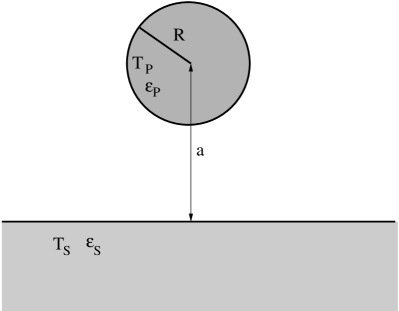
Figure 1: Sketch of a spherical nanoparticle with radius $R$, temperature $T_{{\rm P}}$, and permittivity $\varepsilon_{{\rm P}}$ placed at a distance $a$ above a planar sample with temperature $T_{{\rm S}}$ and permittivity $\varepsilon_{{\rm S}}$.

Now, if an additional spherical particle with radius $R$ is placed at a distance $a$ above the sample, as depicted in Fig. 1, the fluctuating fields $\mathbf{E}_{\rm f}$ and $\mathbf{H}_{\rm f}$ induce an electric dipole moment $\mathbf{p}$ and a Foucault current $\mathbf{j}_{\rm ed}$ within the particle. As emphasized by Chapuis et al. ChapuisEtAl08 , this eddy current $\mathbf{j}_{\rm ed}$ is particularly important for metallic particles. It causes losses inside the particle which can be described by means of an effective magnetic dipole moment $\mathbf{m}_{\rm eff}$, in analogy to the electric dipole moment $\mathbf{p}$. We assume $a\gg R$, so that higher multipoles may be neglected; in principle, this restriction to sufficiently large distances $a$ could be removed by including higher multipoles. Within the dipole approximation, the energy absorbed by the particle can then be written as

$$\langle P_{{\rm S}\rightarrow{\rm P}}\rangle=\langle\dot{\mathbf{p}}\cdot\mathbf{E}_{\rm f}\rangle+\langle\dot{\mathbf{m}}_{\rm eff}\cdot\mathbf{H}_{\rm f}\rangle\;;$$ (1)

the angular brackets denote an ensemble average. For a homogenous and isotropic particle the relations between the induced dipole moments and the fields are given by

$$\mathbf{p}=\varepsilon_{0}\,\mathbf{\alpha}_{\rm p}^{\rm E}\mathbf{E}_{\rm f}$$ (2)

and

$$\mathbf{m}_{\rm eff}=\mu_{0}\,\mathbf{\alpha}_{\rm p}^{\rm H}\mathbf{H}_{\rm f}\;,$$ (3)

where $\mathbf{\alpha}_{\rm p}^{\rm E}$ and $\mathbf{\alpha}_{\rm p}^{\rm H}$ symbolize the electric and magnetic polarizabilities of the particle; $\varepsilon_{0}$ and $\mu_{0}$ are the permittivity and the permeability of the vacuum, respectively. In general, the polarizabilities have a directional dependence and therefore are described by a tensor. For the highly symmetric case of a sphere, this tensor reduces to a scalar multiple of the unit tensor, so that the polarizabilities are represented by scalar values in this case. It is essential to keep in mind that only non-magnetic materials are taken into account here, so that the absorption $\langle\dot{\mathbf{m}}_{\rm eff}\cdot\mathbf{H}_{\rm f}\rangle$ is solely ascribed to the loss due to eddy currents.

With the help of Eqs. (2) and (3) one obtains the expression

$$\begin{split}\langle P_{{\rm S}\rightarrow{\rm P}}\rangle(T_{\rm S})&=\int_{0}^{\infty}\!{\rm d}\omega\,\omega\left[{\rm Im}(\alpha_{{\rm P}}^{\rm E})\varepsilon_{0}\langle\left|\mathbf{E}_{\rm f}\right|^{2}\rangle_{\omega}\right.\\ &\qquad\left.+{\rm Im}(\alpha_{{\rm P}}^{\rm H})\mu_{0}\langle\left|\mathbf{H}_{\rm f}\right|^{2}\rangle_{\omega}\right]\end{split}$$ (4)

for the energy transferred from the sample to the particle ChapuisEtAl08 ; Dorofeyev08 . Here $\langle\left|\mathbf{E}_{\rm f}\right|^{2}\rangle_{\omega}$ denotes the frequency-dependent correlation function of the electric field, i.e., the expectation value of the product of the Fourier transform $\mathbf{E}_{\rm f}(\omega)$ of the fluctuating electric field and its complex conjugate; the correlation function $\langle\left|\mathbf{H}_{\rm f}\right|^{2}\rangle_{\omega}$ of the magnetic field is defined analogously.

Reversely, fluctuating charges inside the sphere of temperature $T_{\rm P}$ give rise to energy transfer from the sphere to the flat surface. The power absorbed within the sample, denoted $\langle P_{{\rm P}\rightarrow{\rm S}}\rangle(T_{\rm p})$, can be calculated in the same manner as $\langle P_{{\rm S}\rightarrow{\rm P}}\rangle(T_{\rm S})$ above. The resulting expression differs from the expression (4) only through the temperature, so that $\langle P_{{\rm P}\rightarrow{\rm S}}\rangle(T_{\rm p})=\langle P_{{\rm S}\rightarrow{\rm P}}\rangle(T_{\rm P})$. As the energy flux $\langle P_{{\rm P}\rightarrow{\rm S}}\rangle$ is directed oppositely to $\langle P_{{\rm S}\rightarrow{\rm P}}\rangle$, the resulting overall heat transfer between the particle and the sample has the form ChapuisEtAl08 ; Dorofeyev08

$$\langle P_{{\rm S}\leftrightarrow{\rm P}}\rangle=\langle P_{{\rm S}\rightarrow{\rm P}}\rangle(T_{\rm S})-\langle P_{{\rm S}\rightarrow{\rm P}}\rangle(T_{\rm P})\;.$$ (5)

The correlation functions $\langle\left|\mathbf{E}_{\rm f}\right|^{2}\rangle_{\omega}$ and $\langle\left|\mathbf{H}_{\rm f}\right|^{2}\rangle_{\omega}$ in Eq. (4) are known from fluctuational electrodynamics RytovEtAl89 . If one assumes that the sample occupies the infinite half space $z\leq 0$, as in Ref. JoulainEtAl05 , one gets

$$\begin{split}&\langle E_{{\rm f},i}\,E_{{\rm f},i}^{*}\rangle_{\omega}=\Theta(\omega,T_{\rm S})\frac{2\omega}{\pi\varepsilon_{0}c^{2}}\biggl{\{}\\ &\qquad\int\limits_{\kappa<k_{0}}\!\!\!\frac{{\rm d}^{2}\kappa}{(2\pi)^{2}}\frac{1}{4k_{z0}}\biggl{[}\bigl{(}\mathbf{e}_{\perp}\otimes\mathbf{e}_{\perp}\bigr{)}_{ii}\bigl{(}1-|r_{\perp}|^{2}\bigr{)}\\ &\qquad\qquad\qquad\quad\,\,\,\,+\bigl{(}\mathbf{e}_{\parallel}^{\rm pr}\otimes\mathbf{e}_{\parallel}^{\rm pr}\bigr{)}_{ii}\bigl{(}1-|r_{\parallel}|^{2}\bigr{)}\biggr{]}\\ &\quad+\int\limits_{\kappa>k_{0}}\!\!\!\frac{{\rm d}^{2}\kappa}{(2\pi)^{2}}\frac{{\rm e}^{-2\gamma\,a}}{2\gamma}\biggl{[}{\rm Im}(r_{\perp})\,\bigl{(}\mathbf{e}_{\perp}\otimes\mathbf{e}_{\perp}\bigr{)}_{ii}\\ &\qquad\qquad\qquad\qquad+{\rm Im}(r_{\parallel})\bigl{(}\mathbf{e}_{\parallel}^{\rm ev}\otimes\mathbf{e}_{\parallel}^{\rm ev}\bigr{)}_{ii}\biggr{]}\biggr{\}}\end{split}$$ (6)

for the electric correlation function, where

$$\Theta(\omega,T)=\frac{\hbar\omega}{{\rm e}^{\hbar\omega\beta}-1}$$ (7)

is the Bose function with the inverse temperature $\beta=1/(k_{\rm B}T)$. Moreover, the unit vectors

$$\begin{split}\mathbf{e}_{\perp}&:=\frac{1}{\kappa}\left(-k_{y},k_{x},0\right)^{\rm t}\\ \mathbf{e}_{\parallel}^{\rm pr}&:=\frac{1}{k_{0}\kappa}\left(k_{x}k_{z0},k_{y}k_{z0},\kappa^{2}\right)^{\rm t}\\ \mathbf{e}_{\parallel}^{\rm ev}&:=\frac{1}{k_{0}\kappa}\left(k_{x}\gamma,k_{y}\gamma,\kappa^{2}\right)^{\rm t}\end{split}$$ (8)

have been introduced, writing $\kappa^{2}=k_{x}^{2}+k_{y}^{2}$ together with $k_{z0}=\sqrt{k_{0}^{2}-\kappa^{2}}$ and $\gamma=\sqrt{\kappa^{2}-k_{0}^{2}}$. As usual, $k_{0}=\omega/c$, where $c$ is the velocity of light in vacuum. In addition, we write

$$\begin{split}r_{\perp}&=\frac{k_{z0}-k_{z}}{k_{z0}+k_{z}}\\ r_{\parallel}&=\frac{\varepsilon_{\rm S}k_{z0}-k_{z}}{\varepsilon_{\rm S}k_{z0}+k_{z}}\end{split}$$ (9)

for the Fresnel reflection coefficients, with $k_{z}=\sqrt{\varepsilon k_{0}^{2}-\kappa^{2}}$. The first integral in Eq. (6), with $\kappa<k_{0}$, describes the propagating part of the fluctuating field, whereas the second integral with $\kappa>k_{0}$ describes the evanescent part. The expression for $\langle H_{{\rm f},i}H_{{\rm f},i}^{*}\rangle_{\omega}$ is obtained from Eq. (6) by interchanging $r_{\perp}\leftrightarrow r_{\parallel}$ and $\frac{1}{\varepsilon_{0}}\leftrightarrow\frac{1}{\mu_{0}}$, due to a corresponding symmetry of the electric and magnetic Green’s functions.

Knowing the correlation functions above a half space, the mean power absorbed by the particle above a planar surface can be calculated from Eq. (4), provided the polarizabilities $\alpha_{\rm P}^{\rm E}$ and $\alpha_{\rm P}^{\rm H}$ are given. In the case of a spherical particle of radius $R$ these quantities can be derived from Mie scattering theory BohrHuff . Denoting the particle’s relative permittivity as $\varepsilon_{\rm P}$, and introducing the dimensionless variables $x=k_{0}R$ and $y=\sqrt{\varepsilon_{\rm P}}k_{0}R$, one finds ChapuisEtAl08b ; BohrHuff

$$\begin{split}\alpha_{\rm P}^{\rm E}&=2\pi R^{3}\frac{\left(2\varepsilon_{\rm P}+1\right)\left(\sin(y)-y\cos(y)\right)-y^{2}\sin(y)}{\left(\varepsilon_{\rm P}-1\right)\left(\sin(y)-y\cos(y)\right)+y^{2}\sin(y)}\\ \alpha_{\rm P}^{\rm H}&=\frac{\pi R^{3}}{3}\left[\frac{\left(x^{2}-6\right)}{y^{2}}\!\!\left(y^{2}+3y\cot(y)-3\right)-\frac{2x^{2}}{5}\right]\end{split}$$ (10)

for $x\ll 1$, implying that the particle’s radius should be small compared to the dominant thermal wavelength, $R\ll\lambda_{\rm th}$. If we demand even $|y|\ll 1$, meaning that the radius be smaller than the skin depth at thermal frequencies, the above expressions reduce to

$$\alpha_{\rm P}^{\rm E} =4\pi\,R^{3}\frac{\varepsilon_{\rm P}-1}{\varepsilon_{\rm P}+2}\;,$$ (11)

$$\alpha_{\rm P}^{\rm H} =\frac{2\pi}{15}R^{3}\left(k_{0}R\right)^{2}\left(\varepsilon_{\rm P}-1\right)\;.$$ (12)

Evidently, the expression for $\alpha_{\rm P}^{\rm E}$ equals the well known Clausius-Mossotti formula.

Before proceeding, we specify the relevant orders of magnitude. For bulk metals the relative permittivity is well described by the Drude model AshcroftMermin76

$$\varepsilon=1-\frac{\omega_{p}^{2}}{\omega\left(\omega+{\rm i}\omega_{\tau}\right)}\;.$$ (13)

For gold at room temperature the plasma frequency is $\omega_{p}=1.4\times 10^{16}\;\text{s}^{-1}$, while the relaxation rate figures as $\omega_{\tau}=3.3\times 10^{13}\;\text{s}^{-1}$. Taking the thermal frequency $\omega_{\rm th}\approx 10^{14}\;\text{s}^{-1}$ one then finds $(\sqrt{|\epsilon|}k_{0})^{-1}\approx 21$ nm, setting a rough upper limit to the radius of a gold sphere for which the expressions (11) and (12) may still hold with reasonable accuracy. When treating such minuscule particles we have to modify the Drude permittivity (13) in order to account for surface scattering, since the bulk mean free path of the electrons, which is about $42$ nm for gold, reaches the same order of magnitude as the spheres’ diameters. For spherical particles of radius $R$ the required correction is achieved by the replacement TomGri

$$\omega_{\tau}\to\widetilde{\omega}_{\tau}=\frac{3}{4}\frac{v_{F}}{R}\;,$$ (14)

where $v_{F}$ is the Fermi velocity. Taking $v_{F}=1.4\times 10^{6}$ m/s for gold, and setting $R=20$ nm, we obtain $\widetilde{\omega}_{\tau}=5.3\times 10^{13}\;\text{s}^{-1}$, less than two times the bulk value. On the other hand, size quantization effects become essential only for radii below 2 nm, and may therefore be neglected here.

3 Dipole model for ellipsoidally shaped particles

The near-field radiative heat transfer between a flat sample with temperature $T_{\rm S}$ and an ellipsoidally shaped particle with temperature $T_{\rm P}$, as sketched in Fig. 2, can be expressed through equations similar to Eqs. (4) and (5), but instead of employing the expressions $\mathbf{\alpha}_{{\rm P}}^{{\rm E}/{\rm H}}$ for the polarizabilities of a sphere, the proper polarizability tensors for an ellipsoidal particle have to be taken into account.

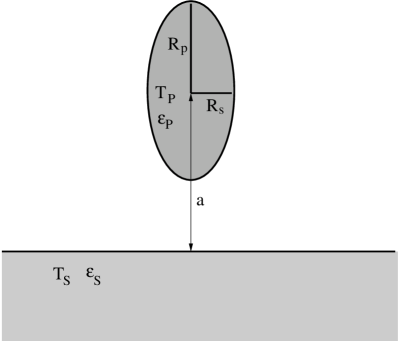
Figure 2: Sketch of a spheroidally shaped particle with semi-axes $R_{{\rm s}}$ and $R_{{\rm p}}$. The semi-axis with length $R_{{\rm p}}$ lies along the spheroid’s axis of rotation.

Denoting the three semi-axes as $R_{x}$, $R_{y}$, $R_{z}$, we require $a\gg\max\{R_{x},R_{y},R_{z}\}\equiv R_{\max}$ to substantiate the dipole approximation, while keeping $R_{\max}$ smaller than the skin depth, thus allowing for approximately homogeneous fields inside the ellipsoids. It is textbook knowledge that the induced dipole moment $\mathbf{p}$ of an ellipsoidal particle is connected with the incident field $\mathbf{E}_{\rm f}$ through the relation LandLif

$$p_{i}=\varepsilon_{0}\,V_{\rm E}\frac{\varepsilon_{\rm P}-1}{1+(\varepsilon_{\rm P}-1)n_{i}}E_{{\rm f},i}$$ (15)

with $V_{\rm E}=\frac{4\pi}{3}R_{x}R_{y}R_{z}$ specifying the volume of the particle, and $\varepsilon_{\rm P}$ its permittivity. It is assumed here that the components of $\mathbf{p}$ and $\mathbf{E}_{\rm f}$ are given in the principal-axis system of the ellipsoid. The polarizability tensor then is diagonal, with diagonal elements given by

$$\alpha_{{\rm E},i}^{\rm E}=V_{\rm E}\frac{\varepsilon_{\rm P}-1}{1+(\varepsilon_{\rm P}-1)n_{i}}\;.$$ (16)

The quantities $n_{i}$ are the so-called depolarization coefficients. They are written as LandLif

$$n_{i}=\frac{R_{x}R_{y}R_{z}}{2}\int_{0}^{\infty}\!\!{\rm d}s\,\frac{1}{(s+R_{i}^{2})R(s)}$$ (17)

with $R(s)=\sqrt{(s+R_{x}^{2})(s+R_{y}^{2})(s+R_{z}^{2})}$. These coefficients depend only on the shape of the ellipsoid, not on its volume. They obey the relations

$$\sum_{i=1}^{3}n_{i}=1\quad\text{and}\quad n_{i}\geq 0\;.$$ (18)

For the special case of a sphere with $R_{x}=R_{y}=R_{z}\equiv R$, Eq. (17) yields $n_{1}=n_{2}=n_{3}=1/3$, so that Eq. (16) correctly reduces to the Clausius-Mossotti formula (11). In the case of spheroid, i.e., of a rotational ellipsoid with two equal semi-axes, $R_{x}=R_{y}\equiv R_{\rm s}$ and $R_{z}\equiv R_{\rm p}$, the coefficients $n_{i}$ take the form LandLif

$$\begin{split}n_{1}(e)&=n_{2}(e)=\frac{1}{2}\bigl{(}1-n_{3}(e)\bigr{)},\\ n_{3}(e)&=\begin{cases}\frac{1-e^{2}}{2e^{3}}\biggl{(}\ln\biggl{(}\frac{1+e}{1-e}\biggr{)}-2e\biggr{)}\;,&R_{\rm s}<R_{\rm p}\\ \frac{1+e^{2}}{e^{3}}\bigl{(}e-\arctan(e)\bigr{)}\;,&R_{\rm s}>R_{\rm p}\;,\end{cases}\end{split}$$ (19)

with

$$e^{2}=\begin{cases}1-\frac{R_{\rm s}^{2}}{R_{\rm p}^{2}}\;,&R_{\rm s}<R_{\rm p}\\ \frac{R_{\rm s}^{2}}{R_{\rm p}^{2}}-1\;,&R_{\rm s}>R_{\rm p}\;.\end{cases}$$ (20)

For calculating the effective magnetic polarizability of an ellipsoid, we follow a strategy outlined by Tomchuk and Grigorchuk TomGri , and use the identity

$$\omega\,{\rm Im}(\alpha_{{\rm E},i}^{\rm H})\mu_{0}\langle\left|H_{\rm f,i}\right|^{2}\rangle_{\omega}={\rm Re}\!\!\int_{V_{\rm E}}\!\!\!\!{\rm d}^{3}r\,\langle\mathbf{j}_{\rm ed}\cdot\mathbf{E_{{\rm f},{\rm ed}}}^{*}\rangle_{\omega}\;,$$ (21)

thus shifting the emphasis from the effective magnetic moment $\mathbf{m}_{\rm eff}$ to a fluctuating eddy field $\mathbf{E_{{\rm f},{\rm ed}}}$. This requires that the material is non-magnetic, so that $\mathbf{m}_{\rm eff}$ is entirely due to eddy currents $\mathbf{j}_{\rm ed}$. The eddy field obeys the equations

$$\nabla\times\mathbf{E}_{{\rm f},{\rm ed}}(\omega) ={\rm i}\omega\mu_{0}\mathbf{H}_{\rm f}(\omega)\;,$$ (22)

$$\nabla\cdot\mathbf{E}_{{\rm f},{\rm ed}}(\omega) =0\;;$$ (23)

in principle, the second equation constitutes a boundary condition for $\mathbf{E}_{{\rm f},{\rm ed}}$. Because we assume $R_{\max}$ to be smaller than the skin depth, $\mathbf{H}_{\rm f}$ can be considered as constant within the volume of the particle, so that the eddy field $\mathbf{E}_{{\rm f},{\rm ed}}$ depends linearly on the spatial coordinates. The resulting relation between $\mathbf{E}_{{\rm f},{\rm ed}}$ and $\mathbf{H}_{\rm f}$ reads TomGri

$$E_{{\rm f},{\rm ed},x}(\omega)={\rm i}\omega\mu_{0}R_{x}^{2}\biggl{(}\frac{zH_{{\rm f},y}(\omega)}{R_{z}^{2}+R_{x}^{2}}-\frac{yH_{{\rm f},z}(\omega)}{R_{x}^{2}+R_{y}^{2}}\biggr{)}\;.$$ (24)

The other components of the electric eddy field are obtained by cyclic permutation of the indices. We emphasize that the underlying assumption of constant fields $\mathbf{H}_{\rm f}$ within the particle is not well fulfilled in cases where the particle’s characteristic linear dimensions are on the order of the skin depth, which is about 21 nm for gold at room temperature. In such cases, the formalism outlined here may still yield the correct orders of magnitude, but not exact numbers.

Next, one has the identity TomGri

$$\mathbf{j}_{\rm ed}(\omega)=\omega\varepsilon_{0}\varepsilon_{\rm P}^{\prime\prime}\mathbf{E}_{{\rm f},{\rm ed}}(\omega)\;,$$ (25)

which relates the induced eddy currents to $\mathbf{E}_{{\rm f},{\rm ed}}$, with $\varepsilon_{\rm P}^{\prime\prime}$ denoting the imaginary part of the particle’s permittivity. Thus, for a spheroid the absorbed energy (21) is found to be

$$\begin{split}&{\rm Re}\int_{V_{\rm E}}\!{\rm d}^{3}r\,\langle\mathbf{j}_{\rm ed}\cdot\mathbf{E_{{\rm f},{\rm ed}}}^{*}\rangle_{\omega}=\frac{\omega^{3}}{c^{2}}\mu_{0}\varepsilon_{{\rm P}}^{\prime\prime}\frac{V_{\rm E}}{10}\times\\ &\biggl{[}\langle|H_{{\rm f},z}|^{2}\rangle_{\omega}R_{\rm s}^{2}+\langle|H_{{\rm f},x}|^{2}+|H_{{\rm f},y}|^{2}\rangle_{\omega}\frac{2R_{\rm s}^{2}R_{\rm p}^{2}}{R_{\rm s}^{2}+R_{\rm p}^{2}}\biggr{]}\;.\end{split}$$ (26)

The effective polarizability is finally read off by comparing this expression with the second term in Eq. (4). Again the polarizability tensor has non-zero entries only on its diagonal, with imaginary parts given by

$$\begin{split}{\rm Im}(\alpha_{{\rm E},x}^{\rm H})&={\rm Im}(\alpha_{{\rm E},y}^{\rm H})=\frac{(k_{0}R_{\rm s})^{2}R_{\rm p}^{2}}{R_{\rm s}^{2}+R_{\rm p}^{2}}\frac{V_{\rm E}\varepsilon_{\rm P}^{\prime\prime}}{5}\;,\\ {\rm Im}(\alpha_{{\rm E},z}^{\rm H})&=\frac{(k_{0}R_{\rm s})^{2}}{10}V_{\rm E}\varepsilon_{\rm P}^{\prime\prime}\;.\end{split}$$ (27)

For a sphere with $R_{\rm s}=R_{\rm p}=R$, both expressions give the correct imaginary part of the Mie formula (12).

Figure 3: Imaginary parts ${\rm Im}(\alpha_{{\rm E},x}^{\rm E})$ and ${\rm Im}(\alpha_{{\rm E},z}^{\rm E})$ of the electric polarizabilities (16) at $\omega_{\rm th}=10^{14}\;\text{s}^{-1}$ for a spheroidal gold particle, and their sum, vs. the ratio $R_{\rm s}/R_{\rm p}$. The spheroid’s volume $V_{\rm E}$ is kept constant at that of a sphere with radius $R=20$ nm; surface scattering is taken into account. Data are normalized by the imaginary part of the electric polarizability ${\rm Im}(\alpha_{\rm P}^{\rm E})$ of the sphere.

Figure 4: Imaginary parts ${\rm Im}(\alpha_{{\rm E},x}^{\rm H})$ and ${\rm Im}(\alpha_{{\rm E},z}^{\rm H})$ of the magnetic polarizabilities (27) at $\omega_{\rm th}=10^{14}\;\text{s}^{-1}$ for a spheroidal gold particle, and their sum, vs. the ratio $R_{\rm s}/R_{\rm p}$. The spheroid’s volume $V_{\rm E}$ is kept constant at that of a sphere with radius $R=20$ nm; surface scattering is taken into account. Data are normalized by the imaginary part of the magnetic polarizability ${\rm Im}(\alpha_{\rm P}^{\rm H})$ of the sphere.

In Figs. 3 and 4 we plot the imaginary parts of the electric and of the magnetic polarizability (16) and (27) at the thermal frequency $\omega_{\rm th}=10^{14}\;\text{s}^{-1}$ against the ratio $R_{\rm s}/R_{\rm p}$, keeping the volume $V_{\rm E}$ constant at that of a sphere with radius $R=20$ nm. The Drude expression (13) has been taken for the permittivity, with the plasma frequency $\omega_{p}=1.4\times 10^{16}\;\text{s}^{-1}$ for gold at room temperature, while surface scattering has been taken into account through the replacement (14), inserting the geometric mean $(R_{\rm s}^{2}R_{\rm p})^{1/3}$ for $R$. This replacement is not fully correct for nonspherical particles TomGri : In principle, one then has different scattering times for different directions, leading to anisotropy of the permittivity. In order to estimate the resulting error, we compare in Fig. 5 the electric absorptivities provided by the Drude permittivity with the simple surface correction (14), and without any correction at all. While the effect of the correction is clearly visible, the general trends are not altered. Hence, a more refined correction taking anisotropy into account should not give drastically different results, at least not in the interval $1/5\leq R_{\rm s}/R_{\rm p}\leq 5$ considered.

Figure 5: Electric absorptivities for spheroidal gold particles with a fixed volume corresponding to that of a sphere with radius $R=20$ nm, both with (corrected) and without (bulk data) surface scattering taken into account.

The curve progressions observed here can be understood intuitively. For the electric polarizability depicted in Fig. 3 the absorptivity ${\rm Im}(\alpha_{{\rm E},z}^{{\rm E}})$ decreases monotonically with increasing ratio $R_{\rm s}/R_{\rm p}$, whereas the absorptivity ${\rm Im}(\alpha_{{\rm E},x}^{{\rm E}})$ increases. For $R_{\rm s}/R_{\rm p}\ll 1$ the spheroidal particle becomes needle-like along the $z$-direction; hence, the polarizability in $z$-direction is much greater than that in $x$- or $y$-direction. On the other hand, when $R_{\rm s}/R_{\rm p}\gg 1$ the spheroid is pancake-like and lies parallel to the $x$-$y$-plane; therefore the polarizability in the directions perpendicular to the $z$-direction dominates.

In the case of the magnetic polarizability shown in Fig. 4 one observes that both ${\rm Im}(\alpha_{{\rm E},x}^{\rm H})$ and ${\rm Im}(\alpha_{{\rm E},z}^{\rm H})$ go to zero in the formal limit $R_{\rm s}/R_{\rm p}\rightarrow 0$. This is clear because these two quantities represent absorptivities caused by eddy currents perpendicular to the $x$- and to the $z$-direction, respectively. Accordingly, for thin needle-like spheroids with $R_{\rm s}/R_{\rm p}\ll 1$ both absorptivities disappear, because no eddy current can arise then. In the opposite case, for $R_{\rm s}/R_{\rm p}\gg 1$, eddy currents can be easily induced perpendicular to the $z$-direction in the pancake-like particle, whereas perpendicular to the $x$-direction no eddy currents occur, as before. Hence, for $R_{\rm s}/R_{\rm p}\rightarrow\infty$ one expects ${\rm Im}(\alpha_{{\rm E},z}^{\rm H})\rightarrow\infty$ and ${\rm Im}(\alpha_{{\rm E},x}^{\rm H})\rightarrow 0$. Since ${\rm Im}(\alpha_{{\rm E},x}^{\rm H})$ is positive for all values of $R_{\rm s}/R_{\rm p}$ and goes to zero in both limiting cases there has to be a maximum, which occurs near $R_{\rm s}/R_{\rm p}=1$, as witnessed by Fig. 4.

4 Radiative heat transfer between an ellipsoidal nanoparticle and a planar surface

In accordance with Sec. 2, the radiative heat transfer from a planar sample to an ellipsoidal nanoparticle is expressed, in analogy to Eq. (4), as

$$\begin{split}\langle P_{{\rm S}\rightarrow{\rm E}}\rangle(T_{\rm S})=\int_{0}^{\infty}\!\!\!{\rm d}\omega\,&\omega\left[{\rm Im}(\alpha_{{\rm E},i}^{\rm E})\varepsilon_{0}\langle\left|E_{{\rm f},i}\right|^{2}\rangle_{\omega}\right.\\ &\left.+{\rm Im}(\alpha_{{\rm E},i}^{\rm H})\mu_{0}\langle\left|H_{{\rm f},i}\right|^{2}\rangle_{\omega}\right]\;,\end{split}$$ (28)

where summation over repeated indices is implied. It is assumed here that the particle is oriented as in Fig. 2, so that the surface normal is parallel to a principal axis of the ellipsoid. As discussed before, this form (28) is quite general, requiring only the specification of the polarizabilities of the nanoparticle, and of the correlation functions of the fluctuating fields above the sample’s surface. The expression $\langle P_{{\rm E}\rightarrow{\rm S}}\rangle$ for the energy flux from the nanoparticle back to the sample can again be obtained from Eq. (28) by substituting the temperature $T_{\rm P}$ for $T_{\rm S}$.

When the specific expressions for a spheroid above a planar sample are inserted into Eq. (28), the propagating modes with $\kappa<k_{0}$ yield the contribution

$$\begin{split}\langle P_{{\rm pr},{\rm S}\rightarrow{\rm E}}&\rangle=\frac{2}{\pi}\int_{0}^{\infty}\!\!\!{\rm d}\omega\,\Theta(\omega,T_{\rm S})k_{0}^{2}\!\!\!\int\limits_{\kappa<k_{0}}\!\!\!\frac{{\rm d}^{2}\kappa}{(2\pi)^{2}}\frac{1}{4k_{z0}}\biggl{\{}\\ &{\rm Im}(\alpha_{{\rm E},x}^{\rm E})\bigl{[}(1-|r_{\perp}|^{2})+\frac{k_{z0}^{2}}{k_{0}^{2}}(1-|r_{\parallel}|^{2})\bigr{]}\\ +&{\rm Im}(\alpha_{{\rm E},z}^{\rm E})\frac{\kappa^{2}}{k_{0}^{2}}(1-|r_{\parallel}|^{2})\\ +&{\rm Im}(\alpha_{{\rm E},z}^{\rm H})\bigl{[}(1-|r_{\parallel}|^{2})+\frac{k_{z0}^{2}}{k_{0}^{2}}(1-|r_{\perp}|^{2})\bigr{]}\\ +&{\rm Im}(\alpha_{{\rm E},x}^{\rm H})\frac{\kappa^{2}}{k_{0}^{2}}(1-|r_{\perp}|^{2})\biggr{\}}\;.\end{split}$$ (29)

This reduces correctly to the known result for a sphere by setting $R_{\rm s}=R_{\rm p}=R$:

$$\begin{split}&\langle P_{{\rm pr},{\rm S}\rightarrow{\rm P}}\rangle=\frac{2}{\pi}\int_{0}^{\infty}\!\!\!{\rm d}\omega\,\Theta(\omega,T_{\rm S})k_{0}^{2}\int\limits_{\kappa<k_{0}}\!\!\!\frac{{\rm d}^{2}\kappa}{(2\pi)^{2}}\frac{1}{4k_{z0}}\\ &\times\biggl{\{}{\rm Im}(\alpha_{{\rm P}}^{{\rm E}}+\alpha_{{\rm P}}^{{\rm H}})\bigl{[}(1-|r_{\parallel}|^{2})+(1-|r_{\perp}|^{2})\bigr{]}\biggr{\}}\;.\end{split}$$ (30)

Observe that sum of the polarizabilities figures here, because $\varepsilon_{0}\langle|\mathbf{E}_{\rm f}|^{2}\rangle_{\omega}=\mu_{0}\langle|\mathbf{H}_{\rm f}|^{2}\rangle_{\omega}$ for the propagating modes. Accordingly, the relative size of ${\rm Im}(\alpha_{{\rm P}}^{{\rm E}})$ and ${\rm Im}(\alpha_{{\rm P}}^{{\rm H}})$ determines whether the radiative heat transfer is dominated by the electric or by the magnetic part. From Eqs. (29) and (30) one can calculate the heat radiated by an ellipsoidal or a spherical nanoparticle in the absence of the sample Martynenko2005 by simply setting $|r_{\perp}|=|r_{\parallel}|=0$ and inserting the temperature $T_{\rm P}$ instead of $T_{\rm S}$.

The heat transfer mediated by the evanescent modes with $\kappa>k_{0}$ from the sample to the spheroidal particle takes the form

$$\begin{split}\langle P_{{\rm ev},{\rm S}\rightarrow{\rm E}}\rangle&=\frac{2}{\pi}\int_{0}^{\infty}\!\!\!{\rm d}\omega\,\Theta(\omega,T_{\rm S})\,k_{0}^{2}\!\!\int\limits_{\kappa>k_{0}}\!\!\!\frac{{\rm d}^{2}\kappa}{(2\pi)^{2}}\frac{{\rm e}^{-2\gamma a}}{2\gamma}\\ &\biggl{\{}{\rm Im}(\alpha_{{\rm E},x}^{\rm E})\bigl{[}{\rm Im}(r_{\perp})+\frac{\gamma^{2}}{k_{0}^{2}}{\rm Im}(r_{\parallel})\bigr{]}\\ &+{\rm Im}(\alpha_{{\rm E},z}^{\rm E})\frac{\kappa^{2}}{k_{0}^{2}}{\rm Im}(r_{\parallel})\\ &+{\rm Im}(\alpha_{{\rm E},x}^{\rm H})\bigl{[}{\rm Im}(r_{\parallel})+\frac{\gamma^{2}}{k_{0}^{2}}{\rm Im}(r_{\perp})\bigr{]}\\ &+{\rm Im}(\alpha_{{\rm E},z}^{\rm H})\frac{\kappa^{2}}{k_{0}^{2}}{\rm Im}(r_{\perp})\biggr{\}}\;.\end{split}$$ (31)

Again this result leads directly to the corresponding expression for a sphere ChapuisEtAl08 :

$$\begin{split}\langle P_{{\rm ev},{\rm S}\rightarrow{\rm P}}\rangle&=\int_{0}^{\infty}\!\!\!{\rm d}\omega\,\Theta(\omega,T_{\rm S})\,k_{0}^{2}\!\!\!\int\limits_{\kappa>k_{0}}\!\!\!\frac{{\rm d}^{2}\kappa}{(2\pi)^{2}}\frac{{\rm e}^{-2\gamma a}}{2\gamma}\biggl{\{}\\ &{\rm Im}(\alpha_{{\rm P}}^{{\rm E}})\bigl{[}{\rm Im}(r_{\perp})+\frac{2\kappa^{2}-k_{0}^{2}}{k_{0}^{2}}{\rm Im}(r_{\parallel})\bigr{]}\\ +&{\rm Im}(\alpha_{{\rm P}}^{{\rm H}})\bigl{[}{\rm Im}(r_{\parallel})+\frac{2\kappa^{2}-k_{0}^{2}}{k_{0}^{2}}{\rm Im}(r_{\perp})\bigr{]}\biggr{\}}\;.\end{split}$$ (32)

Note that in general one has $\varepsilon_{0}\langle|\mathbf{E}_{\rm f}|^{2}\rangle_{\omega}\neq\mu_{0}\langle|\mathbf{H}_{\rm f}|^{2}\rangle_{\omega}$ for the evanescent modes. In contrast to the transfer by propagating modes, this implies that the magnetic contribution to the heat transfer, which is proportional to ${\rm Im}(\alpha_{{\rm P}}^{{\rm H}})$, can dominate the electric one ChapuisEtAl08 even if ${\rm Im}(\alpha_{{\rm P}}^{{\rm E}})>{\rm Im}(\alpha_{{\rm P}}^{{\rm H}})$.

In the quasi-static regime, i.e., for distances $a$ even smaller than the substrate skin depth, one has $\kappa\gg\sqrt{|\epsilon|}k_{0}$, so that Eq. (31) leads to the approximation

$$\begin{split}\langle P_{{\rm ev},{\rm S}\rightarrow{\rm E}}\rangle&\approx\frac{2}{\pi}\int_{0}^{\infty}\!\!\!{\rm d}\omega\,\Theta(\omega,T_{\rm S})\,k_{0}^{2}\!\!\int_{0}^{\infty}\!\frac{{\rm d}\kappa}{2\pi}\frac{\kappa^{2}{\rm e}^{-2\kappa a}}{k_{0}^{2}}\\ &\times\biggl{\{}{\rm Im}(\alpha_{{\rm E},x}^{\rm E}+\alpha_{{\rm E},z}^{\rm E}){\rm Im}(r_{\parallel})\\ &\quad+{\rm Im}(\alpha_{{\rm E},x}^{\rm H}+\alpha_{{\rm E},z}^{\rm H}){\rm Im}(r_{\perp})\biggr{\}}\;.\end{split}$$ (33)

Furthermore, using the approximate expressions

$${\rm Im}(r_{\parallel}) \approx\frac{2\varepsilon_{\rm S}^{\prime\prime}}{|\varepsilon_{\rm S}+1|^{2}}\;,$$ (34)

$${\rm Im}(r_{\perp}) \approx\frac{\varepsilon_{\rm S}^{\prime\prime}k_{0}^{2}}{4\kappa^{2}}$$ (35)

for the imaginary parts of the reflection coefficients, the integration over the wave number $\kappa$ can be carried out, giving

$$\begin{split}\langle P_{{\rm ev},{\rm S}\rightarrow{\rm E}}\rangle&\approx\frac{2}{\pi^{2}}\int_{0}^{\infty}\!\!\!{\rm d}\omega\,\Theta(\omega,T_{\rm S})\\ &\times\biggl{\{}{\rm Im}(\alpha_{{\rm E},x}^{\rm E}+\alpha_{{\rm E},z}^{\rm E})\frac{\varepsilon_{\rm S}^{\prime\prime}}{|\varepsilon_{\rm S}+1|^{2}}\frac{1}{(2a)^{3}}\\ &\quad+{\rm Im}(\alpha_{{\rm E},x}^{\rm H}+\alpha_{{\rm E},z}^{\rm H})\frac{k_{0}^{2}\varepsilon_{\rm S}^{\prime\prime}}{32a}\biggr{\}}\;.\end{split}$$ (36)

As expected, in the quasi-static regime one has $\langle P^{\rm E}_{{\rm ev},{\rm S}\rightarrow{\rm E}}\rangle\propto a^{-3}$ for the electric and $\langle P^{\rm H}_{{\rm ev},{\rm S}\rightarrow{\rm E}}\rangle\propto a^{-1}$ for the magnetic contribution; these power laws are the same as those for a sphere. Since the sums ${\rm Im}(\alpha_{{\rm E},x}^{\rm E}+\alpha_{{\rm E},z}^{\rm E})$ and ${\rm Im}(\alpha_{{\rm E},x}^{\rm H}+\alpha_{{\rm E},z}^{\rm H})$ appear in the frequency integral, one may expect that in this regime $\langle P_{{\rm ev},{\rm S}\rightarrow{\rm E}}\rangle$ behaves like the imaginary part of the sum of the polarizabilities at the thermal frequency when $R_{\rm s}$ and $R_{\rm p}$ are varied.

It needs to be stressed, however, that this approximate result (36) has to be taken with some caution, since the required short particle-sample distances may conflict with those required by the dipole approximation.

5 Discussion

Now we study the shape dependence of the radiative heat transfer between a spheroidal nanoparticle and a planar sample numerically, on the basis of the full expressions (29) and (31). To this end, we assume the temperatures $T_{\rm P}=100\,{\rm K}$ for the particle and $T_{\rm S}=300\,{\rm K}$ for the sample. The permittivity of the sample is described by the bulk Drude model (13) with parameters for gold; that of the particle by the Drude expresson with the plasma frequency of gold, and with the relaxation rate adapted to surface scattering, as before. Since we are interested in the variation of the heat transfer caused by alterations of the shape of the nanoparticle, we vary the ratio $R_{\rm s}/R_{\rm p}$ in such a way that the volume $V_{\rm E}$ of the respective spheroidal nanoparticle equals the volume $V_{\rm P}$ of a sphere with radius $R=20$ nm. We estimate that the range $1/5\leq R_{\rm s}/R_{\rm p}\leq 5$ is about the largest that is still compatible with the dipole approximation, and restrict ourselves to this interval.

Figure 6: Electric contribution $P_{\rm E}^{\rm E}$ to the radiative heat transfer between a spheroidal gold particle with temperature $T_{\rm P}=100\,{\rm K}$ and a planar gold surface with temperature $T_{\rm S}=300\,{\rm K}$, normalized to the corresponding value $P_{\rm P}^{\rm E}$ for a sphere. When the ratio $R_{\rm s}/R_{\rm p}$ is varied, the particle’s volume is kept constant at that of a sphere with radius $R=20$ nm. Line styles distinguish data for particle-sample distances ranging from $50\,{\rm nm}$ to $2000\,{\rm nm}$.

In Fig. 6 we depict the electric contribution to the total heat transfer $P_{\rm E}^{\rm E}$ vs. $R_{\rm s}/R_{\rm p}$ for several distances $a$ between $50$ nm and $2000$ nm, normalized to the corresponding energy transfer $P_{\rm P}^{\rm E}$ between the isochoric sphere and the sample. Evidently, for small distances the curves of $P_{\rm E}^{\rm E}/P_{\rm P}^{\rm E}$ actually resemble those of ${\rm Im}(\alpha_{{\rm E},x}^{\rm E}+\alpha_{{\rm E},z}^{\rm E})$ in Fig. 3, as may have been conjectured from the quasi-static approximation (36), notwithstanding its somewhat shaky justification. On the other hand, for relatively large distances the progression of $P_{\rm E}^{\rm E}/P_{\rm P}^{\rm E}$ is similar to that of ${\rm Im}(\alpha_{{\rm E},z}^{\rm E})$ alone. This behavior stems from the fact that in the latter regime, i.e., at distances such that the propagating modes dominate the heat transfer, one has $\langle|E_{z,{\rm pr}}|^{2}\rangle\gg\langle|E_{x,{\rm pr}}|^{2}+|E_{y,{\rm pr}}|^{2}\rangle$, as documented in Fig. 7. In contrast, in the near-field regime where the evanescent modes dominate the transfer one finds $\langle|E_{z,{\rm ev}}|^{2}\rangle=\langle|E_{x,{\rm ev}}|^{2}+|E_{y,{\rm ev}}|^{2}\rangle$, so that ${\rm Im}(\alpha_{{\rm E},x}^{\rm E})$ and ${\rm Im}(\alpha_{{\rm E},z}^{\rm E})$ contribute in equal measure there.

Figure 7: Ratios $\langle|E_{x}|^{2}+|E_{y}|^{2}\rangle/\langle|E_{z}|^{2}\rangle$ (full line) and $\langle|H_{x}|^{2}+|H_{y}|^{2}\rangle/\langle|H_{z}|^{2}\rangle$ (dashed line) above a semi-infinite planar gold sample at $T_{\rm S}=300\,{\rm K}$, as function of the distance $a$.

Analogously, we plot in Fig. 8 the normalized magnetic contribution $P_{\rm E}^{\rm H}/P_{\rm P}^{\rm H}$ to the total heat transfer, for distances $a$ extending from $50$ nm up to $5000$ nm. Similar to the electric case, in the near-field regime the graphs of $P_{\rm E}^{\rm H}/P_{\rm P}^{\rm H}$ resemble that of ${\rm Im}(\alpha_{{\rm E},x}^{\rm H}+\alpha_{{\rm E},z}^{\rm H})$ previously shown in Fig. 4, since $\langle|H_{z,{\rm ev}}|^{2}\rangle=\langle|H_{x,{\rm ev}}|^{2}+|H_{y,{\rm ev}}|^{2}\rangle$ for small distances (see Fig. 7). On the other hand, for relatively large distances $a$ the plots of $P_{\rm E}^{\rm H}/P_{\rm P}^{\rm H}$ are quite similar to that of ${\rm Im}(\alpha_{{\rm E},x}^{\rm H})$ alone, since then $\langle|H_{z,{\rm pr}}|^{2}\rangle\ll\langle|H_{x,{\rm pr}}|^{2}+|H_{y,{\rm pr}}|^{2}\rangle$.

Figure 8: Magnetic contribution $P_{\rm E}^{\rm H}$ to the radiative heat transfer between a spheroidal gold particle with temperature $T_{\rm P}=100\,{\rm K}$ and a planar gold surface with temperature $T_{\rm S}=300\,{\rm K}$, normalized to the corresponding value $P_{\rm P}^{\rm H}$ for a sphere. When the ratio $R_{\rm s}/R_{\rm p}$ is varied, the particle’s volume is kept constant at that of a sphere with radius $R=20$ nm. Line styles distinguish data for particle-sample distances ranging from $50\,{\rm nm}$ to $5000\,{\rm nm}$.

The ratio of the magnetic to the electric contribution $P_{\rm E}^{\rm H}/P_{\rm E}^{\rm E}$ is drawn in Fig. 9, again for distances from $50$ nm to $5000$ nm. For all distances considered the magnetic contribution to the heat transfer is much greater than the electric one, unless $R_{\rm s}$ is much smaller than $R_{\rm p}$. This fact has been discussed in detail by Chapuis et al. ChapuisEtAl08 for a spherical metallic nanoparticle above a planar metallic sample. Here we find that the curves of the ratio $P_{\rm E}^{\rm H}/P_{\rm E}^{\rm E}$ exhibit a maximum near $R_{\rm s}/R_{\rm p}=1$, so that the dominance of the magnetic part is somewhat less pronounced for nanoparticles with shapes differing from a sphere. For markedly needle-like, prolate particles with a very small ratio $R_{\rm s}/R_{\rm p}$, the graphs suggest that the electric contribution could even dominate the magnetic one, because the induction of Foucault currents would be suppressed by the needle-like shape. We remark that for non-metallic nanoparticles and non-metallic samples the contribution due to induced eddy currents can be neglected anyway, so that for such materials it is always the electric contribution which dominates the heat transfer.

Figure 9: Logarithm of the ratio $P_{\rm E}^{\rm H}/P_{\rm E}^{\rm E}$ of the magnetic to the electric contribution to the heat transfer vs. $R_{\rm s}/R_{\rm p}$, for the situation considered in Figs. 6 and 8.

We conclude from Figs. 6 and 8 that the near-field heat transfer between a metallic nanoparticle and a sample depends to a sizeable extent on the nanoparticle’s shape even when the total radiating volume is kept constant. In the example considered, the electric contribution to the heat transfer is enhanced for strongly prolate spheroids by a factor of about 10 as compared to a perfect sphere, and by a factor of about 4 for strongly oblate ones. On the other hand, the magnetic contribution is substantially reduced in the needle-like case, but exceeds the sphere value by a factor of about 2 for pancake-like particles, always assuming the orientation specified in Fig. 2.

6 Conclusions

We have investigated the radiative heat transfer between a metallic spheroidal nanoparticle and a planar metallic probe for small and large distances, on the basis of the analytical expressions (29) and (31) for the heat transfer mediated by propagating and evanescent modes, respectively. By numerical analysis for the example of a spheroidal gold particle above a gold surface we have investigated in detail the precise shape dependence of the radiative heat transfer in both the near-field and the far-field regime. Furthermore, we have derived the approximate expression (36) for the nonretarded evanescent regime, which provides a qualitative understanding of the numerical results.

Figure 10: Heat transfer between a gold spheroid with temperature $T_{\rm P}=100\,{\rm K}$ and a planar gold surface with temperature $T_{\rm S}=300\,{\rm K}$ separated by $100$ nm. The volume of the spheroid is kept constant at that of a sphere with radius $R=20$ nm when $R_{\rm s}/R_{\rm p}$ is varied. The horizontal line marks the value of the heat current between the isochoric sphere and the sample.

Figure 10 shows the absolute total heat transfer between a gold spheroid with temperature $T_{\rm P}=100\,{\rm K}$ and a planar gold surface with temperature $T_{\rm S}=300\,{\rm K}$ for the separation $a=100$ nm, again fixing the spheroid’s volume at that of a sphere with radius $R=20$ nm when changing the aspect ratio. For $R_{\rm s}/R_{\rm p}=1/5$ the heat transfer between spheroid and sample is only about half of that between sphere and sample, whereas for $R_{\rm s}/R_{\rm p}=5$ the spheroid-sample transfer is roughly two times as efficient as that occurring in the sphere-sample geometry. The very fact that there exists such a marked shape dependence might be of interest for nanoscale thermal engineering, insofar as it appears possible to control the amount of heat transported at nanoscale distances by carefully designing the shapes of both the emitting and the absorbing pieces.

Our discussion is subject to several restrictions: There is the dipole approximation (1) made right at the outset, the assumption of constant fields $\mathbf{H}_{\rm f}$ inside the particle entering into Eq. (24), and the simplified correction (14) for surface scattering. Taken together, these simplifications render our analysis approximate, rather than exact, although they should still capture the essential physics. Further issues that should be investigated in future works concern the possible effects of spatial dispersion ChapuisEtAl08c , and of surface roughness BiehsGreffet09 .

With respect to the problem of quantifying the actual heat transfer in a near-field scanning thermal microscope, our study helps to pin down the error margin. A typical NSThM sensor tip is larger than the nanoparticles considered in our examples, and does possess an internal structure, but again the precise shape of the sensor will influence the heat current it records. In view of our model calculations, we estimate that the values obtained on the grounds of the dipole model under the assumption of an ideal spherical sensor may deviate, in the appropriate distance regime, by up to an order of magnitude from the true values, but probably not by more.

7 Acknowledgments

This work was supported by the Deutsche Forschungsgemeinschaft through Grant No. KI 438/8-1. S.-A. B. gratefully acknowledges a fellowship awarded by the Deutsche Akademie der Naturforscher Leopoldina under Grant No. LPDS 2009-7.

References

• (1) O. Sqalli, I. Utke, P. Hoffmann, and F. Marquis-Weible, J. Appl. Phys. 92, 1078 (2002)
• (2) K. Joulain, J.-P. Mulet, F. Marquier, R. Carminati, and J.-J. Greffet, Surf. Sci. Rep. 57, 59 (2005)
• (3) A. I. Volokitin and B. N. J. Persson, Rev. Mod. Phys. 79, 1291 (2007)
• (4) R. S. DiMatteo, P. Greiff, S. L. Finberg, K. A. Young-Waithe, H. K. Choy, M. M. Masaki, and C. G. Fonstad, Appl. Phys. Lett. 79, 1894 (2001)
• (5) A. Narayanaswamy and G. Chen, Appl. Phys. Lett. 82, 3544 (2003)
• (6) M. Laroche, R. Carminati, and J.-J. Greffet, J. Appl. Phys. 100, 063704 (2006)
• (7) M. Francoeur, M. P. Mengüç, and R. Vaillon, Appl. Phys. Lett. 93, 043109 (2008)
• (8) S. Basu, Z. M. Zhang, and C. J. Fu, Int. J. Energy Res. 33, 1203 (2009)
• (9) S. M. Rytov, Y. A. Kravtsov, and V. I. Tatarskii, Principles of Statistical Radiophysics (Springer, New York, 1989)
• (10) D. Polder and M. van Hove, Phys. Rev. B 4, 3303 (1971)
• (11) M. L. Levin, V. G. Polevoi, and S. M. Rytov, Sov. Phys. JETP 52, 1054 (1980)
• (12) J. J. Loomis and H. J. Maris, Phys. Rev. B 50, 18517 (1994)
• (13) J. B. Pendry, J. Phys.: Condens. Matter 11, 6621 (1999)
• (14) J. L. Pan, Opt. Lett. 25, 369 (2000)
• (15) A. I. Volokitin and B. N. J. Persson, Phys. Rev. B 69, 045417 (2004)
• (16) G. Bimonte, Phys. Rev. Lett. 96, 160401 (2006)
• (17) S.-A. Biehs, Eur. Phys. J. B 58, 423 (2007)
• (18) A. Narayanaswamy and G. Chen, Phys. Rev. B 77, 075125 (2008)
• (19) P.-O. Chapuis, M. Laroche, S. Volz, and J.-J. Greffet, Appl. Phys. Lett. 92, 201906 (2008)
• (20) A. Pérez-Madrid, J. M. Rubí, and L. C. Lapas, Phys. Rev. B 77, 155417 (2008)
• (21) I. A. Dorofeyev, J. Phys. D: Appl. Phys. 31, 600 (1998)
• (22) J.-P. Mulet, K. Joulain, R. Carminati, and J.-J. Greffet, Appl. Phys. Lett. 78, 2931 (2001)
• (23) G. V. Dedkov and A. A. Kyasov, Tech. Phys. 33, 305 (2007)
• (24) P.-O. Chapuis, M. Laroche, S. Volz, and J.-J. Greffet, Phys. Rev. B 77, 125402 (2008)
• (25) A. I. Volokitin and B. N. J. Persson, Phys. Rev. B 63, 205404 (2001)
• (26) I. Dorofeyev, H. Fuchs, B. Gotsmann, and G. Wenning, Phys. Rev. B 60, 9060 (1999)
• (27) C. M. Hargreaves, Phys. Lett. 30A, 491 (1969)
• (28) G. A. Domoto, R. F. Boehm, and C. L. Tien, Trans. ASME, Ser. C: J. Heat Transfer 92, 412 (1970)
• (29) J.-B. Xu, K. Läuger, R. Möller, K. Dransfeld, and I. H. Wilson, J. Appl. Phys. 76, 7209 (1994)
• (30) L. Hu, A. Narayanaswamy, X. Chen, and G. Chen, Appl. Phys. Lett. 92, 133106 (2008)
• (31) A. Narayanaswamy, S. Shen, and G. Chen, Phys. Rev. B 78, 115303 (2008)
• (32) S. Shen, A. Narayanaswamy, and G. Chen, Nano Lett. 9, 2909 (2009)
• (33) E. Rousseau, A. Siria, G. Jourdan, S. Volz, F. Comin, J. Chevrier, and J.-J. Greffet, Nature Photonics 3, 514 (2009)
• (34) W. Müller-Hirsch, A. Kraft, M. T. Hirsch, J. Parisi, and A. Kittel, J. Vac. Sci. Technol. A 17, 1205 (1999)
• (35) A. Kittel, W. Müller-Hirsch, J. Parisi, S.-A. Biehs, D. Reddig, and M. Holthaus, Phys. Rev. Lett. 95, 224301 (2005)
• (36) U. F. Wischnath, J. Welker, M. Munzel, and A. Kittel, Rev. Sci. Instrum. 79, 073708 (2008)
• (37) I. Dorofeyev, Phys. Lett. A 372, 1341 (2008)
• (38) C. F. Bohren and D. R. Huffman, Absorption and Scattering of Light by Small Particles (Wiley Science, New York, 1998)
• (39) N. W. Ashcroft and N. D. Mermin, Solid State Physics (Harcourt, Fort Worth, 1976)
• (40) P. M. Tomchuk and N. I. Grigorchuk, Phys. Rev. B 73, 155423 (2006)
• (41) L. D. Landau and E. M. Lifshitz, Electrodynamics of Continuous Media (Pergamon, Oxford, 1960)
• (42) Yu. V. Martynenko and L. I. Ognev, Tech. Phys. 50, 1522 (2005)
• (43) P.-O. Chapuis, S. Volz, C. Henkel, K. Joulain, and J.-J. Greffet, Phys. Rev. B 77, 035431 (2008)
• (44) S.-A. Biehs and J.-J. Greffet, Near-field heat transfer between a nanoparticle and a rough surface (Preprint, 2009)