Two-channel Kondo physics in odd impurity chains

Abstract

We study odd-membered chains of spin-$\tfrac{1}{2}$ impurities, with each end connected to its own metallic lead. For antiferromagnetic exchange coupling, universal two-channel Kondo (2CK) physics is shown to arise at low energies. Two overscreening mechanisms are found to occur depending on coupling strength, with distinct signatures in physical properties. For strong inter-impurity coupling, a residual chain spin-$\tfrac{1}{2}$ moment experiences a renormalized effective coupling to the leads; while in the weak-coupling regime, Kondo coupling is mediated via incipient single-channel Kondo singlet formation. We also investigate models where the leads are tunnel-coupled to the impurity chain, permitting variable dot filling under applied gate voltages. Effective low-energy models for each regime of filling are derived, and for even-fillings where the chain ground state is a spin singlet, an orbital 2CK effect is found to be operative. Provided mirror symmetry is preserved, 2CK physics is shown to be wholly robust to variable dot filling; in particular the single-particle spectrum at the Fermi level, and hence the low-temperature zero-bias conductance, is always pinned to half-unitarity. We derive a Friedel-Luttinger sum rule and from it show that, in contrast to a Fermi liquid, the Luttinger integral is non-zero and determined solely by the ‘excess’ dot charge as controlled by gate voltage. The relevance of the work to real quantum dot devices, where inter-lead charge-transfer processes fatal to 2CK physics are present, is also discussed. Physical arguments and numerical renormalization group techniques are used to obtain a detailed understanding of these problems.

I Introduction

Non-Fermi liquid (NFL) behavior is famously realised in the two-channel Kondo (2CK) model,Nozières and Blandin (1980) in which a single spin-$\tfrac{1}{2}$ impurity is exchange-coupled to two equivalent but independent metallic conduction bands. Its fascination for theorists is evident in the wide range of techniques applied to the model, including notably the Bethe ansatz,Sacramento and Schlottmann (1989); Andrei and Jerez (1995); Andrei and Destri (1984); Tsvelick and Wiegmann (1984); Zaránd et al. (2002) numerical renormalization groupCragg and Lloyd (1979); Cragg et al. (1980); Pang and Cox (1991); Zaránd et al. (2002); Affleck et al. (1992) and conformal field theoryAffleck et al. (1992); Affleck and Ludwig (1990); Ludwig and Affleck (1991); Affleck and Ludwig (1993) (for a review, see Ref. Cox and Zawadowski, 1998). Such methods have elucidated key aspects of the NFL state arising from ‘overscreening’ of the impurity spin below the low-energy 2CK scale,Nozières and Blandin (1980) $T_{K}^{2CK}$; including exotic physical properties such as a residual entropy of $\tfrac{1}{2}\ln(2)$, and a logarithmically divergent low-temperature magnetic susceptibility, which are symptomatic of the frustration inherent when two conduction channels compete to screen the impurity local moment.Cox and Zawadowski (1998) NFL scaling of the conductance has also been predicted theoreticallyAffleck and Ludwig (1993); Cox and Zawadowski (1998); Oreg and Goldhaber-Gordon (2003); Pustilnik et al. (2004); Tóth et al. (2007), and measured experimentallyPotok et al. (2007) in quantum dots, with its square-root temperature dependence being a characteristic signature of the 2CK phase.

This is all of course in marked contrast to standard Fermi liquid (FL) behavior,Hewson (1993) arising for example in the single-channel spin-$\tfrac{1}{2}$ Kondo or Anderson modelsHewson (1993) (realised in practice in e.g. ultrasmall quantum dotsGoldhaber-Gordon et al. (1998); Cronenwett et al. (1998)). Here, the dot spin is completely screened by a single bath of conduction electrons. The impurity entropy is in consequence quenched on the lowest energy scales, and the susceptibility is constant.Hewson (1993) Such systems are characterised by a unitarity zero-bias conductance, with a quadratic temperature dependence at low-energies.Pustilnik and Glazman (2004)

But the NFL physics of the 2CK model is delicate: finite channel-asymmetry and/or inter-channel charge transfer ultimately drive any real system out of the NFL regime,Cox and Zawadowski (1998); Affleck and Ludwig (1990) to a FL ground state. The exquisite tunability of quantum dot devicesKouwenhoven et al. (1997) allows manipulation of such perturbations; indeed couplings can be fine-tuned via application of gate voltages to effectively eliminate channel-asymmetry. However, tunnel-coupling in such systems must result in some degree of charge transfer between the metallic ‘leads’. This is of course responsible for the predominance of single-channel Kondo physics in real quantum dot systems.

Suppressing inter-channel charge transfer allows for the emergence of 2CK physics at intermediate temperatures/energies, although the instability of the 2CK fixed point to charge-transfer means that an incipient NFL state forming at $T\sim T_{K}^{2CK}$ is subsequently destroyed below a FL crossover scale $T_{\text{FL}}$. Observation of NFL behavior at higher temperatures thus depends on a clear separation of scales, $T_{\text{FL}}\ll T_{K}^{2CK}$. This was achieved recently Potok et al. (2007) through use of an interacting lead tuned to the Coulomb blockade regime, and to date it is the only unambiguous experimental demonstration of the 2CK effect. Alternatively, sequential tunneling through several coupled dots should suppress charge transfer between leads,Zaránd et al. (2006) and this could be exploited to access 2CK physics; although the interplay between spin and orbital degrees of freedom in coupled quantum dot systems can also generate new physics, as well known both theoreticallyJones et al. (1988); Jones and Varma (1989); Zaránd et al. (2006); Sela and Affleck (2009a, b); Vojta et al. (2002); Garst et al. (2004); Galpin et al. (2005); Mitchell et al. (2006); Boese et al. (2002); Cornaglia and Grempel (2005); Žitko and Bonča (2007a); Žitko (2010); Oguri and Hewson (2005); Kuzmenko et al. (2006); Žitko et al. (2006); Mitchell et al. (2009); Numata et al. (2009); Žitko and Bonča (2007b); Žitko and Bonča (2008); Vernek et al. (2009); Mitchell and Logan (2010); Ferrero et al. (2007) and experimentally.Blick et al. (1996); van der Wiel et al. (2000); Jeong et al. (2001); Vidan et al. (2005); Schröer et al. (2007); Rogge and Haug (2008); Grove-Rasmussen et al. (2008); Roch et al. (2008); Gaudreau et al. (2009); Granger et al. (2010); Potok et al. (2007)

In light of the above, we here consider odd-membered coupled quantum dot chains (each end of which is connected to its own metallic lead), and demonstrate that 2CK physics is indeed generally accessible in these systems. In models where the couplings are of pure exchange type, we show that the low-energy behavior is described by the channel-asymmetric two-channel Kondo model,Cox and Zawadowski (1998) with pristine 2CK physics surviving down to the lowest energy scales in the mirror-symmetric systems of most interest. Such models are considered in Sec. II, where analytic predictions are confirmed and supplemented by use of Wilson’s numerical renormalization group (NRG) techniqueWilson (1975); Krishnamurthy et al. (1980); Bulla et al. (2008); Peters et al. (2006); Weichselbaum and von Delft (2007) (for a recent review see Ref. Bulla et al., 2008). In particular, universal scaling of thermodynamic and dynamic properties is demonstrated for odd chains of different length, and for systems with different coupling strengths. While the underlying 2CK physics of such systems is shown to be robust for finite antiferromagnetic exchange coupling, we find that the mechanism of overscreening differs according to whether the inter-impurity coupling is strong or weak. In the former case (Sec. II.1), it is the single lowest spin-$\tfrac{1}{2}$ state of the chain which effectively couples to and is overscreened by the leads; while for weak inter-impurity coupling (Sec. II.2), two-channel Kondo coupling is mediated via incipient single-channel Kondo singlets. Clear signatures of the latter are evident in the behavior of the frequency-dependent t-matrix, results for which are presented and analysed.

In order to investigate conductance across two-channel coupled quantum dot chains, we study in Sec. III a related class of models in which the terminal impurities are Anderson-like quantum levels, tunnel-coupled to their respective metallic leads (although with inter-lead charge transfer still precluded by inter-impurity exchange couplings). In the mirror-symmetric systems considered, we derive effective low-energy 2CK models valid for each regime of electron-filling. Even-occupation filling regimes – where the chain ground state is a spin-singlet – are found in particular to exhibit an orbital 2CK effect, with spin playing the role of a channel index. In consequence, 2CK physics is found to be robust throughout all regimes of electron-filling induced by changes in gate voltage.

Single-particle dynamics for such systems are then considered, and hence conductance (Sec. III.3.1), the S-matrix and associated phase shifts (Sec. III.4); again highlighting the universality arising at low-energies. It is found in particular that the Fermi level value of the $T=0$ single-particle spectrum – and hence the zero-bias conductance – is pinned to a half-unitary value, irrespective of electron-filling. A Friedel-Luttinger sum rule Logan et al. (2009) is then derived in Sec. III.5, relating the Fermi level value of the spectrum to the ‘excess’ charge due to the quantum dot chain, and the Luttinger integral.Luttinger (1960); Luttinger and Ward (1960) By virtue of the spectral pinning, the sum rule relates directly the Luttinger integral to the excess charge/dot filling; in contrast to a Fermi liquid, where it is the Luttinger integral that is ubiquitously ‘pinned’ (to zero),Luttinger (1960); Luttinger and Ward (1960) and the dot filling then determines the value of the spectrum at the Fermi level.Hewson (1993); Langreth (1966)

Finally, in Sec. IV we consider briefly the applicability of our findings to real coupled quantum dot devices. We argue that the effective low-energy model describing such systems is generically a 2CK model with both channel-asymmetry and inter-lead cotunneling charge transfer. Via a suitable basis transformation, one obtains a model in which charge transfer between even and odd channels is eliminated, whence the underlying behavior is readily understood in terms of that of a pure channel-asymmetric 2CK model. The spectrum/t-matrix in a given physical channel is however related via this transformation to a combination of t-matrices in even and odd channels. In the mirror-symmetric case sought experimentally, this leads to the striking conclusion that for sufficiently small but non-vanishing cotunneling charge transfer, the crossover out of the NFL regime is not in fact apparent in conductance measurements, despite the ultimate low-energy physics being that of a Fermi liquid.

II 2CK Heisenberg chains

We consider a chain of $N_{c}$ coupled spin-$\tfrac{1}{2}$ impurities, each end of which is also coupled to its own metallic lead, as illustrated in Fig. 1. To investigate 2CK physics, we study explicitly in this section a system of exchange-coupled spin-$\tfrac{1}{2}$ impurities, where inter-lead charge transfer is eliminated from the outset. For an impurity chain of length $N_{c}$, the full Hamiltonian is thus $H^{N_{c}}=H_{L}+H^{N_{c}}_{\text{c}}+H^{N_{c}}_{\text{K}}$. Here $H_{L}=\sum_{\alpha,\textbf{k},\sigma}\epsilon^{\phantom{\dagger}}_{\textbf{k}}a^{\dagger}_{\alpha\textbf{k}\sigma}a^{\phantom{\dagger}}_{\alpha\textbf{k}\sigma}$ refers to the two equivalent non-interacting metallic leads ($\alpha=L$/$R$), and

$$H^{N_{c}}_{\text{c}}= J\sum_{i=1}^{N_{c}-1}\hat{\textbf{S}}_{i}\cdot\hat{\textbf{S}}_{i+1}$$ (1a)

$$H^{N_{c}}_{\text{K}}= J_{KL}\hat{\textbf{S}}_{1}\cdot\hat{\textbf{s}}_{L0}+J_{KR}\hat{\textbf{S}}_{N_{c}}\cdot\hat{\textbf{s}}_{R0}$$ (1b)

where $\hat{\textbf{S}}_{i}$ is a spin-$\tfrac{1}{2}$ operator for impurity $i$, and $\hat{\textbf{s}}_{\alpha 0}$ is the spin density of lead $\alpha=L(R)$ at impurity $1(N_{c})$:

$$\hat{\textbf{s}}_{\alpha 0} =\sum_{\sigma,\sigma^{\prime}}f^{\dagger}_{\alpha 0\sigma}\boldsymbol{\sigma}_{\sigma\sigma^{\prime}}f^{\phantom{\dagger}}_{\alpha 0\sigma^{\prime}}$$ (2a)

$$f^{\dagger}_{\alpha 0\sigma} =\tfrac{1}{\sqrt{N}}\sum_{\textbf{k}}a^{\dagger}_{\alpha\textbf{k}\sigma}~{},$$ (2b)

with $\boldsymbol{\sigma}$ the Pauli matrices and $f^{\dagger}_{\alpha 0\sigma}$ the creation operator for the ‘0’-orbital of the $\alpha=L$/$R$ Wilson chain ($N\rightarrow\infty$ is the number of orbitals/$\mathbf{k}$-states in the chain).

In the following, we focus on odd-$N_{c}$ chains, with antiferromagnetic (AF) exchange couplings for both the intra-chain Heisenberg exchange, $J>0$, and the Kondo exchanges, $J_{K\alpha}>0$. [We do not consider here even-$N_{c}$ chains, where the generic low-energy physics is quite different and in essence that of the two-impurity Kondo model]. We also consider both the channel symmetric case, $J_{KR}=J_{KL}$, as well as the more general case where channel asymmetry is present, $J_{KR}\neq J_{KL}$. The simplest member of the family, $N_{c}=1$, is of course the classic single-spin 2CK model,Nozières and Blandin (1980); Cox and Zawadowski (1998) while variants of the $N_{c}=3$ trimer have also been considered previously.Kuzmenko et al. (2006); Žitko et al. (2006); Mitchell et al. (2009); Numata et al. (2009); Žitko and Bonča (2007b); Žitko and Bonča (2008); Vernek et al. (2009); Mitchell and Logan (2010) We show below that an effective single-spin 2CK model results in all cases, whence universal 2CK physics is expected on the lowest energy scales in the channel-symmetric case; albeit that the mechanism by which the effective two-channel coupling arises is rather different in the strong and weak inter-impurity coupling regimes.

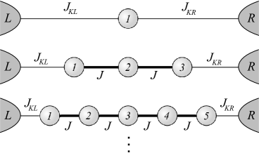
Figure 1: Schematic illustration of odd-membered impurity chains, each end of which is coupled to its own metallic lead.

II.1 Strong inter-impurity coupling

We consider first the case where the inter-impurity exchange couplings $J$ are sufficiently large that only the ground state of the isolated spin chain is relevant in constructing the effective low-energy model upon coupling to the leads. As detailed in Sec. II.2, this means in practice $J\gtrsim T_{K,\alpha}^{1CK}$, with $T_{K,\alpha}^{1CK}$ the scale for single-channel Kondo quenching of a terminal spin to lead $\alpha$, arising in the “uncoupled” $J=0$ limit. The lowest state of an AF-coupled odd-membered spin-$\tfrac{1}{2}$ chain is of course a spin doublet, the components of which we label as $|N_{c};S^{z}=\pm\tfrac{1}{2}\rangle$. All other states are at least $\mathcal{O}(J/N_{c})$ higher in energy.

II.1.1 Effective 2CK model

To leading order in $J_{K\alpha}$, the low-energy model is then obtained simply by projecting into the reduced Hilbert space of the lowest doublet for a chain of length $N_{c}$, using

$$\hat{1}_{N_{c}}=\sum_{S^{z}}|N_{c};S^{z}\rangle\langle N_{c};S^{z}|.$$ (3)

The resultant Hamiltonian $H^{N_{c}}_{\text{eff}}=\hat{1}_{N_{c}}H^{N_{c}}_{c}\hat{1}_{N_{c}}$ follows as

$$\begin{split}H^{N_{c}}_{\text{eff}}=\tfrac{1}{2}J_{K}\hat{1}_{N_{c}}&(\hat{\textbf{S}}_{1}+\hat{\textbf{S}}_{N_{c}})\hat{1}_{N_{c}}\cdot(\hat{\textbf{s}}_{L0}+\hat{\textbf{s}}_{R0})\\ +\tfrac{1}{2}\delta_{K}\hat{1}_{N_{c}}&(\hat{\textbf{S}}_{1}+\hat{\textbf{S}}_{N_{c}})\hat{1}_{N_{c}}\cdot(\hat{\textbf{s}}_{L0}-\hat{\textbf{s}}_{R0})\end{split}$$ (4)

where $J_{K}=\tfrac{1}{2}(J_{KL}+J_{KR})$ and $\delta_{K}=\tfrac{1}{2}(J_{KL}-J_{KR})$, and we use the symmetry $\hat{1}_{N_{c}}\hat{\textbf{S}}_{1}\hat{1}_{N_{c}}=\hat{1}_{N_{c}}\hat{\textbf{S}}_{N_{c}}\hat{1}_{N_{c}}$.

In the absence of a magnetic field, $\uparrow/\downarrow$ spin symmetry implies $\hat{P}_{\uparrow\downarrow}|N_{c};S^{z}\rangle=\gamma|N_{c};-S^{z}\rangle$, where $\hat{P}_{\uparrow\downarrow}$ permutes simultaneously all up and down spins, and $\gamma=\pm 1$ only since $\hat{P}_{\uparrow\downarrow}^{2}=\hat{1}$.Mitchell and Logan (2010) Together with $\hat{P}_{\uparrow\downarrow}\hat{S}^{z}_{i}=-\hat{S}^{z}_{i}\hat{P}_{\uparrow\downarrow}$, it follows directly that

$$\begin{split}\langle N_{c};S^{z}&|\hat{S}_{1}^{z}+\hat{S}_{N_{c}}^{z}|N_{c};S^{z}\rangle\\ =-\langle N_{c};-S^{z}&|\hat{S}_{1}^{z}+\hat{S}_{N_{c}}^{z}|N_{c};-S^{z}\rangle\propto S^{z}\end{split}$$ (5)

(as $|N_{c};S^{z}\rangle$ is a spin doublet). Such matrix elements appear in the $z$-component of the contraction in Eq. 4, and by spin isotropy an effective model of 2CK form results:

$$H^{N_{c}}_{\text{eff}}=J_{K,N_{c}}^{\text{eff}}\hat{\textbf{S}}\cdot(\hat{\textbf{s}}_{L0}+\hat{\textbf{s}}_{R0})+\delta^{\text{eff}}_{K,N_{c}}\hat{\textbf{S}}\cdot(\hat{\textbf{s}}_{L0}-\hat{\textbf{s}}_{R0})$$ (6)

where $\hat{\textbf{S}}$ is a spin-$\tfrac{1}{2}$ operator for the lowest chain doublet, defined by $\hat{S}^{z}=\sum_{S^{z}}|N_{c};S^{z}\rangle S^{z}\langle N_{c};S^{z}|$ and $\hat{S}^{\pm}=|N_{c};\pm\tfrac{1}{2}\rangle\langle N_{c};\mp\tfrac{1}{2}|$. The effective couplings are given by

$$J_{K,N_{c}}^{\text{eff}}=\langle N_{c};+\tfrac{1}{2} |\hat{S}_{1}^{z}+\hat{S}_{N_{c}}^{z}|N_{c};+\tfrac{1}{2}\rangle J_{K},$$ (7a)

$$\delta_{K,N_{c}}^{\text{eff}}=\langle N_{c};+\tfrac{1}{2} |\hat{S}_{1}^{z}+\hat{S}_{N_{c}}^{z}|N_{c};+\tfrac{1}{2}\rangle\delta_{K}.$$ (7b)

Numerical evaluation of Eq. 7 for odd $N_{c}$ yields an AF effective coupling, $J_{K,N_{c}}^{\text{eff}}>0$, which is renormalized with respect to the bare coupling and diminishes as the chain length increases, as shown in Table I.

Table 1: Effective couplings

$N_{c}$	$J_{K,N_{c}}^{\text{eff}}/J_{K}^{\phantom{\dagger}}$
1	$1$
3	$\tfrac{2}{3}$
5	$0.51...$
7	$0.42...$

Hence, for sufficiently low temperatures $T\ll J/N_{c}$, the low-energy behavior of the system is equivalent to the single-spin 2CK model.Cox and Zawadowski (1998) In the $L/R$ mirror-symmetric case, $J_{KL}=J_{KR}$ ($\delta_{K}=\delta_{K}^{\text{eff}}=0$), the stable $T=0$ fixed point (FP) is then the infrared 2CK FP. The lowest spin-$\tfrac{1}{2}$ state of the impurity chain is thus overscreened by conduction electrons; giving rise to a residual entropy of $S_{\text{imp}}=\tfrac{1}{2}\text{ln}(2)~{}~{}(k_{B}=1)$, a hallmark of the NFL 2CK ground state.Cox and Zawadowski (1998) Overscreening sets in below a characteristic scale $T_{K}^{2CK}$, given from perturbative scalingNozières and Blandin (1980) as

$$T_{K}^{2CK}\sim J_{K,N_{c}}^{\text{eff}}\exp(-1/\rho J_{K,N_{c}}^{\text{eff}}),$$ (8)

where $\rho=1/(2D)$ is the lead density of states per orbital (assumed to be uniform) and $2D$ is the bandwidth.

By contrast, when strict $L/R$ mirror symmetry is broken via distinct exchange couplings to the two leads, $J_{KL}\neq J_{KR}$ (ie. $\delta_{K}\neq 0$), the 2CK FP is destabilized in the full model Eq. 1. This behavior is of course well-known from the single-spin 2CK model with channel anisotropy,Nozières and Blandin (1980); Cox and Zawadowski (1998); Sacramento and Schlottmann (1989); Andrei and Jerez (1995); Affleck et al. (1992) where the impurity local moment is fully screened by conduction electrons in the more strongly coupled lead, and a Fermi liquid ground state results. For $\delta_{K}>0$, under renormalization on reduction of the temperature/energy scale, the system flows to strong coupling (SC) with the left lead ($J_{KL}\rightarrow\infty$) while the right lead decouples ($J_{KR}\rightarrow 0$).Nozières and Blandin (1980); Cox and Zawadowski (1998); Sacramento and Schlottmann (1989); Andrei and Jerez (1995); Affleck et al. (1992) The stable $T=0$ FP thus depends on the sign of $\delta_{K}$, with ‘SC:L’ describing the lowest energy behavior for $\delta_{K}>0$ while ‘SC:R’ is stable for $\delta_{K}<0$. The mirror-symmetric case, $\delta_{K}=0$, is as such the quantum critical point separating phases where a Kondo singlet forms in either the $L$ or $R$ lead.

In the full model, effective single-channel Kondo screening characteristic of flow to the Fermi liquid FP in channel-asymmetric systems, sets in below a characteristic scale which can likewise be obtained from perturbative scaling:Nozières and Blandin (1980)

$$T_{K}^{SC}\sim J_{K,N_{c}}^{>}\exp(-1/\rho J_{K,N_{c}}^{>}),$$ (9)

where $J_{K,N_{c}}^{>}=J_{K,N_{c}}^{\text{eff}}+|\delta_{K,N_{c}}^{\text{eff}}|$ is the effective coupling between the lowest chain doublet state and the more strongly-coupled lead.

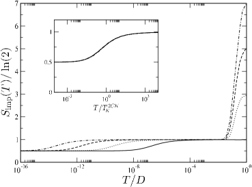
Figure 2: Entropy $S_{\text{imp}}(T)/\ln(2)$ vs $T/D$ for chains of length $N_{c}=1,3,5,7$ (solid, dotted, dashed and dot-dashed lines respectively) in the large inter-impurity coupling regime. Shown for $\rho J=0.15$ and $\rho J_{K}=0.075$ in the $L/R$-symmetric limit $\delta_{K}=0$. Inset: scaling collapse onto the universal 2CK curve.

II.1.2 NRG results: symmetric case

The above picture indicates that in the mirror symmetric case, $\delta_{K}=0$, the lowest energy behavior for all odd chains should be that of the single-spin 2CK model,Cox and Zawadowski (1998) but with renormalized effective couplings (Eq. 7 and Table 1) and hence from Eq. 8 a reduced 2CK scale, $T_{K}^{2CK}$.

We now analyze the full model, Eq. 1, for odd $N_{c}=1,3,5,7$ using Wilson’s NRG technique,Wilson (1975); Krishnamurthy et al. (1980); Bulla et al. (2008) employing a complete basis set of the Wilson chainPeters et al. (2006) to calculate the full density matrix.Peters et al. (2006); Weichselbaum and von Delft (2007) Calculations here are typically performed using an NRG discretization parameter $\Lambda=3$, retaining the lowest $N_{s}=4000$ states per iteration. We consider first the impurity contributionKrishnamurthy et al. (1980); Bulla et al. (2008) to thermodynamics $\langle\hat{\Omega}\rangle_{\mathrm{imp}}=\langle\hat{\Omega}\rangle-\langle\hat{\Omega}\rangle_{0}$, with $\langle\hat{\Omega}\rangle_{0}$ denoting a thermal average in the absence of the impurity chain. We focus in particular on the entropy, $S_{\text{imp}}(T)$, and the uniform spin susceptibility, $\chi_{\text{imp}}(T)=\langle(\hat{S}^{z})^{2}\rangle_{\mathrm{imp}}/T$ (here $\hat{S}^{z}$ refers to the spin of the entire system); the temperature dependences of which provide clear signatures of the underlying FPs reached under renormalization on progressive reduction of the temperature/energy scale.Krishnamurthy et al. (1980); Bulla et al. (2008)

Fig. 2 shows representative NRG results for the $T$-dependence of the entropy, for odd chains with $N_{c}=1,3,5,7$. At high temperatures the impurities are effectively uncoupled, so the chain contribution to the entropy is $S_{\text{imp}}=N_{c}\ln(2)$, as seen clearly from Fig. 2. On the scale of $T\sim J/N_{c}$, all but the lowest chain doublet are projected out, the entropy then dropping as expected to $\ln(2)$ in all cases. Renormalization group (RG) flow to this local moment (LM) FPNozières and Blandin (1980); Krishnamurthy et al. (1980) marks the regime of validity of the effective single-spin 2CK model, Eq. 6. The local moment is then overscreenedNozières and Blandin (1980); Cox and Zawadowski (1998) by symmetric coupling to the two leads on an exponentially-small scale, $T_{K}^{2CK}$; the $T=0$ residual entropy in all cases being $\tfrac{1}{2}\ln(2)$. $T_{K}^{2CK}$ itself is determined in practice from $S_{\text{imp}}(T_{K}^{2CK})=\tfrac{3}{4}\ln(2)$ (suitably between the characteristic LM and 2CK FP values). The exponential reduction of the 2CK scale with increasing chain length (evident in Fig. 2) is expected from Eq. 8, which depends on $N_{c}$ through the effective coupling given in Table 1. The inset shows the data rescaled in terms of $T/T_{K}^{2CK}$. The low-temperature behavior of all odd chains collapse to the universal scaling curve for the single-spin 2CK model (ie. the $N_{c}=1$ case, solid line), likewise known from e.g. the Bethe ansatz solution,Sacramento and Schlottmann (1989); Andrei and Jerez (1995); Andrei and Destri (1984); Tsvelick and Wiegmann (1984); Zaránd et al. (2002) confirming the mapping of the full model to Eq. 6.

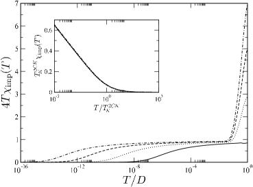
Figure 3: Spin susceptibility $4T\chi_{\text{imp}}(T)$ vs $T/D$ for the same parameters as Fig. 2. Inset: scaling collapse of $\chi_{\text{imp}}(T)$ itself onto the universal 2CK curve, with characteristic NFL form $T_{K}^{2CK}\chi_{\text{imp}}(T)=\alpha\ln(T_{K}^{2CK}/T)$.

The above FP structure and energy scales also naturally show up in the magnetic susceptibility, as seen in Fig. 3. At the highest temperatures, $T\chi_{\text{imp}}=\tfrac{1}{4}N_{c}$, as expectedHewson (1993); Krishnamurthy et al. (1980) for $N_{c}$ free spins. Flow to the LM FP on the scale $T\sim J/N_{c}$ is again clearly evident in the drop to $T\chi_{\text{imp}}=\tfrac{1}{4}$, corresponding to the expected Curie law behavior. On the scale $\sim T_{K}^{2CK}$, the susceptibility drops to $T\chi_{\text{imp}}=0$, which remains its $T=0$ value. The inset shows $T_{K}^{2CK}\chi_{\text{imp}}$ vs $T/T_{K}^{2CK}$, showing scaling collapse to the universal single-spin 2CK curve, and demonstrating the characteristic NFL logarithmic divergenceCox and Zawadowski (1998) of the susceptibility $\chi_{\text{imp}}$ itself on approaching the 2CK FP.

We turn now to dynamics, in particular the low-energy Kondo resonance embodied in the spectrum $D\rho_{K}(\omega)\equiv D\rho_{K,\alpha}(\omega)=-\pi\rho_{T}\text{Im}[t_{\alpha}(\omega)]$; where $t_{\alpha}(\omega)\equiv t(\omega)$ is the t-matrixHewson (1993) for the $\alpha=L/R$ lead (equivalent by symmetry for $\delta_{K}=0$), and $\rho_{T}=N\rho$ is the total lead density of states. Using equation of motion techniquesHewson (1993); Zubarev (1960) yields

$$\pi\rho_{T}t_{\alpha}(\omega)=\frac{\pi}{4}\rho J_{K\alpha}^{2}\tilde{G}_{\alpha i}(\omega)$$ (10)

with $i=1$ for $\alpha=L$ and $i=N_{c}$ for $\alpha=R$, where

$$\tilde{G}_{\alpha i}(\omega)=\langle\langle\hat{S}_{i}^{-}f^{\phantom{\dagger}}_{\alpha 0\downarrow}+\hat{S}_{i}^{z}f^{\phantom{\dagger}}_{\alpha 0\uparrow};\hat{S}_{i}^{+}f^{\dagger}_{\alpha 0\downarrow}+\hat{S}_{i}^{z}f^{\dagger}_{\alpha 0\uparrow}\rangle\rangle_{\omega}^{\phantom{\dagger}}$$ (11)

and $\langle\langle\hat{A};\hat{B}\rangle\rangle_{\omega}^{\phantom{\dagger}}$ is the Fourier transform of the retarded correlator $\langle\langle\hat{A}(t_{1});\hat{B}(t_{2})\rangle\rangle=-i\theta(t_{1}-t_{2})\langle\{\hat{A}(t_{1}),\hat{B}(t_{2})\}\rangle$. The correlator in Eq. 11 can be calculated directly within NRG,Peters et al. (2006); Weichselbaum and von Delft (2007); Bulla et al. (2008) hence enabling access to the spectrum $D\rho_{K}(\omega)$. However, an alternative expression for the t-matrix can be obtained in the spirit of Ref. Bulla et al., 1998, and in the wide flat-band case considered here is simply

$$\pi\rho_{T}t_{\alpha}(\omega)=-i\left[1+\left(\frac{2}{\pi\rho J_{K\alpha}}\right)^{2}\frac{G_{\alpha 0}(\omega)}{\tilde{G}_{\alpha i}(\omega)}\right]^{-1}$$ (12)

where $G_{\alpha 0}(\omega)=\langle\langle f^{\phantom{\dagger}}_{\alpha 0\sigma};f^{\dagger}_{\alpha 0\sigma}\rangle\rangle_{\omega}^{\phantom{\dagger}}$ is the Green function for the ‘0’-orbital of the $\alpha=L/R$ Wilson chain.Wilson (1975) The quotient of correlators in Eq. 12 is found to improve greatly numerical accuracy, and is employed in the following.

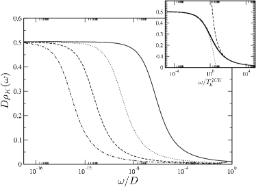
Figure 4: $T=0$ spectrum $D\rho_{K}(\omega)$ vs $\omega/D$, for the same parameters as Fig. 2. Inset: vs $\omega/T_{K}^{2CK}$, showing collapse to the scaling spectrum for odd chains. Grey dotted line: low-$|\omega|/T_{K}^{2CK}\ll 1$ asymptotic behavior $D\rho_{K}(\omega)=\tfrac{1}{2}[1-b(|\omega|/T_{K}^{2CK})^{1/2}]$; grey dashed line: high-$|\omega|/T_{K}^{2CK}\gg 1$ scaling behavior, $D\rho_{K}(\omega)=A/[\ln^{2}(|\omega|/T_{K}^{2CK})+B]$.

Fig. 4 shows the resultant spectrum $D\rho_{K}(\omega)$ vs $\omega/D$ for chains of length $N_{c}=1,3,5,7$ with the same parameters as Figs. 2 and 3 (noting that $\rho_{K}(\omega)=\rho_{K}(-\omega)$ since the model, Eq. 1, is particle-hole symmetric). The low-energy form of each spectrum naturally reflects RG flow in the vicinity of the 2CK FP, as studied also in a variety of different models which exhibit 2CK behavior.Affleck and Ludwig (1993); Žitko and Bonča (2007b); Johannesson et al. (2005); Bradley et al. (1999); Tóth and Zaránd (2008); Mitchell and Logan (2010); Anders (2005). In particular, for all odd chains, a half-unitarity value is seen to arise at the Fermi level, $D\rho_{K}(\omega=0)=\tfrac{1}{2}$; and collapse to the universal single-spin 2CK scaling spectrum is clearly evident in the inset to Fig. 4. The leading low-frequency asymptotic behavior is $D\rho_{K}(\omega)=\tfrac{1}{2}[1-b(|\omega|/T_{K}^{2CK})^{1/2}]$ (in marked contrast to the form $[1-a(|\omega|/T_{K})^{2}]$ characteristicHewson (1993) of RG flow near a Fermi liquid FP); and with which the numerics agree well for $\omega\ll T_{K}^{2CK}$. At high frequencies $\omega\gg T_{K}^{2CK}$ by contrast, the leading asymptotic behavior of the scaling spectrum is $D\rho_{K}(\omega)=A/[\ln^{2}(|\omega|/T_{K}^{2CK})+B]$, which behavior is common to other models in which spin-flip scattering processes are important at high energies,Dickens and Logan (2001); Galpin et al. (2009) such as the single-channel Anderson or Kondo models.

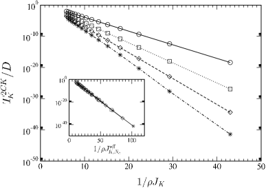
Figure 5: Kondo temperature $T_{K}^{2CK}/D$ vs $1/\rho J_{K}$ for chains of length $N_{c}=1,3,5,7$ (circles, squares, diamonds and stars respectively, with lines as guide to the eye) and common exchange coupling $\rho J=0.15$. Inset: scaling collapse to common linear form when plotted vs $1/\rho J_{K,N_{c}}^{\text{eff}}$ (given by Eq. 7).

Finally, we consider the evolution of the 2CK scale itself as the impurity-lead coupling is varied in the mirror-symmetric case, shown vs $1/\rho J_{K}$ in Fig. 5 for chains of length $N_{c}=1,3,5,7$. An exponential dependence of the 2CK scale on the impurity-lead coupling is expected from Eq. 8, and seen clearly in the main panel. The differing slopes reflect the renormalization of the bare Kondo coupling $J_{K}\rightarrow J_{K,N_{c}}^{\text{eff}}$ with increasing impurity chain length (Table 1); collapse to common linear behavior being observed in the inset where the 2CK scales are plotted vs $1/\rho J_{K,N_{c}}^{\text{eff}}$, establishing thereby quantitative agreement with Eqs. 7,8 and Table 1, and hence the mapping to the effective 2CK model, Eq. 6.

II.1.3 NRG results: asymmetric case

We turn now to the channel-asymmetric case, $J_{KL}\neq J_{KR}$ (ie. $\delta_{K}\neq 0$). The effective model Eq. 6 should describe the low-energy behavior of all odd chains, so the rich physics of the asymmetric single-spin 2CK modelNozières and Blandin (1980); Cox and Zawadowski (1998); Sacramento and Schlottmann (1989); Andrei and Jerez (1995); Affleck et al. (1992) is thus expected for $T\ll J/N_{c}$. As discussed above, breaking $L/R$ mirror symmetry is a relevant perturbationAffleck et al. (1992) to the 2CK FP, so FL physics will arise generically on the lowest energy scales. Indeed, in the limit of maximal asymmetry $J_{K}=\delta_{K}$, the right lead is completely decoupled in Eq. 6; pristine single-channel Kondo (1CK) screening by the left lead then results below a single-channel scale $T_{K}^{1CK}$. For $\delta_{K}\ll T_{K}^{1CK}$, however, RG flow in the vicinity of the 2CK FP strongly affects the behavior at higher temperatures/energies.Nozières and Blandin (1980); Cox and Zawadowski (1998); Sacramento and Schlottmann (1989); Andrei and Jerez (1995); Affleck et al. (1992) This is indeed seen in Fig. 6(A), where the entropy $S_{\text{imp}}(T)$ vs $T/D$ is shown for a representative system with $N_{c}=3$, $\rho J=0.25$, $\rho J_{K}=0.125$, varying $\rho\delta_{K}=10^{-1}$, $10^{-2}$, $10^{-3}$, $10^{-4}$, $10^{-5}$, $10^{-6}$, $10^{-7}$ [lines (a)–(g)], successively approaching the quantum critical point at the symmetric limit, $\delta_{K}=0$: line (h). The scale $T_{K}^{1CK}$ (for which $\rho J_{K}=\rho\delta_{K}$) is $\rho T_{K}^{1CK}\approx 10^{-3}$ here; and sets the scale for the crossover from ‘large’ to ‘small’ channel asymmetry ($\rho\delta_{K}\gg\rho T_{K}^{1CK}$ and $\ll\rho T_{K}^{1CK}$ respectively).

At the highest temperatures the three impurity spins are effectively free, yielding trivially a common entropy $S_{\text{imp}}=3\ln(2)$. As $T$ is lowered, all but the lowest trimer doublet state is projected out, heralding flow to the LM FP, with characteristicNozières and Blandin (1980); Krishnamurthy et al. (1980) entropy $S_{\text{imp}}=\ln(2)$. For large channel asymmetry [e.g. lines (a),(b)], RG flow is then directly to the SC:L FP: the impurity spin is fully screenedNozières and Blandin (1980); Cox and Zawadowski (1998); Sacramento and Schlottmann (1989); Andrei and Jerez (1995); Affleck et al. (1992) by formation of a Kondo singlet with conduction electrons in the left lead ($\delta_{K}>0$) below an effective single-channel Kondo scale $T_{K}^{SC}$, and hence $S_{\text{imp}}=0$ for $T\ll T_{K}^{SC}$. The Kondo scale itself is given by Eq. 9 in the large $\delta_{K}$ regime,not with an effective Kondo coupling $J_{K,N_{c}=3}^{\text{eff}}=\tfrac{2}{3}(J_{K}+|\delta_{K}|)$ for $N_{c}=3$ (see Table 1).

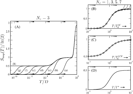
Figure 6: (A): Entropy $S_{\text{imp}}(T)/\ln(2)$ vs $T/D$ on progressively approaching the transition, for $N_{c}=3$. Shown for fixed $\rho J=0.25$ and $\rho J_{K}=0.125$, varying $\rho\delta_{K}=10^{-1}$, $10^{-2}$, $10^{-3}$, $10^{-4}$, $10^{-5}$, $10^{-6}$, $10^{-7}$ [lines (a)–(g)], with the symmetric point $\rho\delta_{K}=0$ shown as line (h). (B): Scaling collapse to the 1CK curve (circles) for strong channel asymmetry, $\rho\delta_{K}=10^{-1}$ and $10^{-2}$, with $N_{c}=1,3,5,7$. (C): For small asymmetry ($\rho\delta_{K}=10^{-6}$ and $10^{-7}$), and $N_{c}=1,3,5,7$. Showing universality in the LM$\rightarrow$2CK FP crossover, on rescaling in terms of $T/T_{K}^{2CK}$; compared directly to the symmetric 2CK scaling curve (circles). (D): Same data as (C), now rescaled in terms of $T/T^{\star}$; showing universal crossover from the 2CK FP ($S_{\text{imp}}/\ln 2=\tfrac{1}{2}$) to the stable SC:L FP ($S_{\text{imp}}=0$).

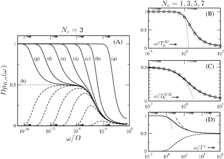
Figure 7: (A): Spectra $D\rho_{K,L}(\omega)$ (solid lines) and $D\rho_{K,R}(\omega)$ (dashed) vs $\omega/D$ on progressively approaching the transition for $N_{c}=3$, using the same parameters as in Fig. 6. (B): Collapse of $D\rho_{K,L}(\omega)$ to the 1CK scaling spectrum (circles) in the strongly asymmetric limit, $\rho\delta_{K}=10^{-1}$ and $10^{-2}$, for $N_{c}=1,3,5,7$. The dotted line shows the asymptotic low-$|\omega|/T_{K}^{SC}$ FL behavior $D\rho_{K,L}(\omega)=1-a(|\omega|/T_{K}^{SC})^{2}$. (C): For small asymmetry ($\rho\delta_{K}=10^{-6}$ and $10^{-7}$ for $N_{c}=1,3,5,7$), universal behavior arising on rescaling $D\rho_{K,\alpha}(\omega)$ for both $\alpha=L/R$ in terms of $\omega/T_{K}^{2CK}$, as compared with the symmetric 2CK scaling curve (circles). The dotted line shows the asymptotic ($T^{\star}\ll|\omega|\ll T_{K}^{2CK}$) NFL behavior $D\rho_{K,\alpha}(\omega)=\tfrac{1}{2}[1-b(|\omega|/T_{K}^{2CK})^{1/2}]$. (D): Same data rescaled in terms of $T/T^{\star}$, showing the universal low-temperature crossover for $D\rho_{K,L}(\omega)$ (solid lines) and $D\rho_{K,R}(\omega)\equiv 1-D\rho_{K,L}(\omega)$ (dashed). The $T^{\star}\ll|\omega|\ll T_{K}^{2CK}$ asymptotic behavior $D\rho_{K,L}(\omega)=\tfrac{1}{2}[1+c(|\omega|/T^{\star})^{-1/2}]$ is shown as a dot-dashed line; while for $|\omega|\ll T^{\star}$ FL behavior results, $D\rho_{K,L}(\omega)=1-d(|\omega|/T^{\star})^{2}$ (dotted line).

In the case of smaller channel asymmetry, $\rho\delta_{K}\ll\rho T_{K}^{1CK}$, RG flow to the stable Fermi liquid SC:L FP occurs via the critical FP, which is of course the 2CK FP. The chain spin-$\tfrac{1}{2}$ associated with the LM FP is then fully screened in a two-stage process (Fig. 6(A)). All such systems flow first to the 2CK FP on a common scale $T_{K}^{2CK}$, given by Eq. 8. The entropy thus drops to $S_{\text{imp}}=\tfrac{1}{2}\ln(2)$, symptomaticCox and Zawadowski (1998) of overscreening; before being quenched completely below a scale $T\sim T^{\star}$ characterizingNozières and Blandin (1980); Cox and Zawadowski (1998); Sacramento and Schlottmann (1989); Andrei and Jerez (1995); Affleck et al. (1992) the flow to the SC:L FP (with $T^{*}$ defined in practice by $S_{\text{imp}}(T^{*})=\tfrac{1}{4}\ln 2$). A clear $S_{\text{imp}}=\tfrac{1}{2}\ln(2)$ plateau is thus seen for lines (d)–(g) in Fig. 6(A), with $T^{\star}$ diminishing rapidly as the transition is approached. The evolution of $T^{\star}$ on varying $\delta_{K}$ for different odd chains is itself studied in Fig. 8, below; and the result in the small-$|\delta_{K}|$ regime is a characteristic power-law decay,

$$T^{\star}~{}\overset{\delta_{K}\rightarrow 0^{\pm}}{\sim}~{}{\cal{A}}|\delta_{K}|^{\nu}~{}~{}~{}~{}~{}~{}:\nu=2$$ (13)

with exponent $\nu=2$, and common amplitudes $\cal{A}$ on approaching the transition at $\delta_{K}=0$ from either side (as guaranteed by symmetry). Eq. 13 generalizes the known resultCox and Zawadowski (1998); Sacramento and Schlottmann (1989); Andrei and Jerez (1995) for the channel-anisotropic single-spin 2CK model, and is expected from the mapping of the full chain model (Eq. 1) onto the effective model, Eq. 6.

We now turn to the scaling behavior of the entropy for chains of different length, as demonstrated by the three universal curves given in panels (B)–(D) of Fig. 6. First, in Fig. 6(B) for $N_{c}=1,3,5,7$, we show strongly asymmetric systems ($\rho\delta_{K}\gg\rho T_{K}^{1CK}$) with $\rho\delta_{K}=10^{-1}$ and $10^{-2}$. The data clearly collapse to common scaling form when scaled in terms of $T/T_{K}^{SC}$, indicative of universal one-stage quenching from the LM to the SC:L FP. Results for the single-channel spin-$\tfrac{1}{2}$ Kondo model are also shown (circles), confirming that the crossover is characterized by effective single-channel Kondo screening.

The situation is more subtle for weakly asymmetric systems $\rho\delta_{K}\ll\rho T_{K}^{1CK}$, where two-stage quenching occurs from the LM FP, through the 2CK FP, to the fully quenched SC:L FP. As now shown, each of these stages separately exhibit universal scaling, in terms of the two distinct low-energy scales $T_{K}^{2CK}$ and $T^{\star}$ respectively. In Figs. 6(C),(D) for $N_{c}=1,3,5,7$, systems close to the transition are shown. To determine the full universal curves, it is of course essential to obtain good scale separation of $T_{K}^{2CK}$ and $T^{\star}$: here $T_{K}^{2CK}/T^{\star}>10^{8}$.

In Fig. 6(C), results are rescaled in terms of $T/T_{K}^{2CK}$. Collapse to the universal scaling curve for the symmetric single-spin 2CK model (shown separately, circles) is seen clearly; the crossover from the LM FP ($S_{\text{imp}}=\ln 2$) to the 2CK FP ($S_{\text{imp}}=\tfrac{1}{2}\ln 2$) being as such determined by the 2CK scale $T_{K}^{2CK}$. By contrast, the universality of the crossover from the unstable 2CK FP to the stable low-$T$ SC:L FP with $S_{\text{imp}}=0$, is shown in Fig. 6(D). Here, on rescaling in terms of $T/T^{\star}$ the data collapse to a universal form controlled by the low-energy scale $T^{*}$, itself vanishing (Eq. 13) as the quantum critical point $\delta_{K}=0$ is approached.

The FP structure and energy scales naturally show up also in dynamical quantities, such as the scattering t-matrix, and hence the spectra $D\rho_{K,\alpha}(\omega)$. These are considered in Fig. 7. In panel (A), again for $N_{c}=3$, we focus on $D\rho_{K,L}(\omega)$ (solid lines) and $D\rho_{K,R}(\omega)$ (dashed) for systems with the same parameters as Fig. 6(A). Results for $\delta_{K}<0$ are not shown, the $\alpha=L$ and $R$ spectra simply being exchanged under the transformation $\delta_{K}\leftrightarrow-\delta_{K}$.

$N_{c}=3$ chains with $\rho\delta_{K}=10^{-1}$ and $10^{-2}$ [strong channel-asymmetry, lines (a) and (b)], show a characteristic resonance in the left-channel spectrum, $D\rho_{K,L}(\omega)$, on the scale $|\omega|\sim T_{K}^{SC}$; with the Fermi level value in particular being $D\rho_{K,L}(0)=1$. This is the single-channel Kondo resonance; as is physically natural for these strongly channel-asymmetric cases because effective single-channel Kondo screening is operative,Affleck et al. (1992) with the behavior thus expected to be that of the single-channel Kondo or Anderson models.Hewson (1993) In the particle-hole symmetric limit of the latter, the Friedel sum ruleLangreth (1966) guarantees satisfaction of the unitarity limit ($D\rho_{K,L}(0)=1$); and in the scaling regime $|\omega|\ll J/N_{c}$ one expects the entire one-channel scaling spectrum to be recovered. This is considered in panel (B), where results for $N_{c}=1,3,5,7$ and $\rho\delta_{K}=10^{-1}$ and $10^{-2}$ are shown, rescaled in terms of $\omega/T_{K}^{SC}$: essentially perfect agreement is seen with the universal scaling spectrum for the single-channel Kondo model (shown separately as circles). For $T_{K}^{SC}\ll|\omega|\ll J/N_{c}$ the characteristic $D\rho_{K,L}(\omega)\sim A/[\ln^{2}(|\omega|/T_{K}^{SC})+B]$ behavior typical of ‘high’ energy spin-flip scatteringDickens and Logan (2001); Galpin et al. (2009) arises; while for $|\omega|\ll T_{K}^{SC}$ canonical Fermi liquid behavior,Hewson (1993) $D\rho_{K,L}(\omega)=1-a(|\omega|/T_{K}^{SC})^{2}$, occurs as expected.

Spectra for the right lead/channel, $D\rho_{K,R}(\omega)$ [dashed lines (a) and (b) of panel (A)], are similarly described by the leading $\sim 1/\ln^{2}(|\omega|/T_{K}^{SC})$ logarithms at high energies. However, the upward renormalization of the effective Kondo coupling to the right lead — and hence RG flow towards the SC:R FP — is cut off at $|\omega|\sim T_{K}^{SC}$, below which frequency the impurity chain local moment becomes fully screened by strong coupling to the left lead. Thus $D\rho_{K,R}(\omega)=0$ for $|\omega|\ll T_{K}^{SC}$, as observed directly from the NRG results in panel (A).

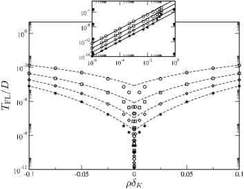
Figure 8: Fermi liquid crossover temperature $T_{\text{FL}}/D$ vs $\rho\delta_{K}$ for chains of length $N_{c}=1,3,5,7$ (circles, squares, diamonds and stars) and couplings $\rho J=0.25$ and $\rho J_{K}=0.125$. For large channel asymmetry, $T_{\text{FL}}\equiv T_{K}^{SC}$: good agreement between the data and Eq. 9 (dashed lines) is seen for each $N_{c}$ in the regime $|\rho\delta_{K}|\gtrsim 0.025$. The inset shows the small asymmetry behavior on a log-log plot. Here $T_{\text{FL}}\equiv T^{\star}$, and the quadratic behavior of Eq. 13 is shown as the solid lines, onto which data fall cleanly for $\rho|\delta_{K}|\lesssim 0.01$.

We now turn to lines (e)–(g) of Fig. 7(A), for $N_{c}=3$ systems with much smaller channel-asymmetry, $\rho\delta_{K}\ll\rho T_{K}^{1CK}$. For both $\alpha=L$ and $R$, a clear half-unitary plateau of $D\rho_{K,\alpha}(\omega)\simeq\tfrac{1}{2}$ arises for $T^{\star}\ll|\omega|\ll T_{K}^{2CK}$, indicative of RG flow near the 2CK FP. For $|\omega|\sim T^{\star}$, however, flow to the Fermi liquid SC:L FP occurs, such that $D\rho_{K,L}(\omega=0)=1$ and $D\rho_{K,R}(\omega=0)=0$ are again satisfied. As was seen from the entropy (Fig. 6), there are two universal scales in this regime associated with the crossover from the LM FP to the 2CK FP [see panel (C)] and from the 2CK FP to the SC:L FP [panel (D)].

In panel (C) of Fig. 7, results are shown for systems of chain length $N_{c}=1,3,5,7$ and small channel asymmetry, $\rho\delta_{K}=10^{-6}$ and $10^{-7}$. Each is rescaled in terms of $\omega/T_{K}^{2CK}$, and collapse to the universal symmetric 2CK curve (circles) is seen in all cases — for both $\alpha=L$ and $R$ spectra. In particular, for $|\omega|\ll T_{K}^{2CK}$ the characteristic NFL behavior is obtained, $D\rho_{K,\alpha}(\omega)=\tfrac{1}{2}[1-b(|\omega|/T_{K}^{2CK})^{1/2}]$ (dotted line).

Finally, panel (D) shows the same data, but rescaled now in terms of $|\omega|/T^{\star}$. Two universal spectra emerge: one for $D\rho_{K,L}(\omega)$ and one for $D\rho_{K,R}(\omega)$. The two scaling spectra are however found to be related simply by $D\rho_{K,R}(\omega)=1-D\rho_{K,L}(\omega)$, so we need consider only $D\rho_{K,L}(\omega)$ (solid line). For $\omega\gg T^{\star}$ the relevant $L/R$ symmetry-breaking operator dominates,Affleck et al. (1992) driving RG flow away from the 2CK FP. Since the scaling dimension of this operatorAffleck et al. (1992) is $\tfrac{1}{2}$, one expects $D\rho_{K,L}(\omega)=\tfrac{1}{2}[1+c(|\omega|/T^{\star})^{-1/2}]$ (as indeed found, dot-dashed line). By contrast, for $|\omega|\ll T^{\star}$, irrelevant operatorsKrishnamurthy et al. (1980); Affleck et al. (1992) affect the RG flow in the vicinity of the stable FL FP, so one expects the leading low-$|\omega|/T^{\star}$ asymptotics to be $D\rho_{K,L}(\omega)=1-d(|\omega|/T^{\star})^{2}$ (dotted line). Good agreement with the numerics is seen in both regimes and for both $\alpha=L/R$ spectra in Fig. 7(D).

As the critical point is approached [$|\delta_{K}|\rightarrow 0$; lines (a)$\rightarrow$(h) in Fig. 7], the spectra fold progressively onto the 2CK spectrum itself [line (h)] down to lower and lower frequencies. The scale $T^{\star}$ describing flow away from the 2CK FP vanishes according to Eq. 13, as evident from the dynamics shown in Fig. 7 (or the thermodynamics in Fig. 6). In Fig. 8 the evolution of the low-energy scale as a function of channel asymmetry, $\rho\delta_{K}$, is examined. Since $T_{K}^{SC}$ is the lowest energy scale of the problem in the large-$|\delta_{K}|$ regime, while $T^{\star}$ is the lowest scale for small $|\delta_{K}|$, we consider the generic crossover scale $T_{\text{FL}}$ in Fig. 8, defined in practice from the entropy via $S_{\text{imp}}(T_{\text{FL}})=\tfrac{1}{4}\ln(2)$; which as such characterizes the flow to the ultimate stable FL FP, and hence complete screening of the impurity spin. $T_{\text{FL}}/D$ is shown vs $\rho\delta_{K}$ for chains of length $N_{c}=1,3,5,7$. The dashed lines in the main panel show comparison to the perturbative result for $T_{K}^{SC}$ given in Eq. 9 (with a prefactor $\mathcal{O}(1)$ for each $N_{c}$ adjusted to fit the numerics). The inset shows the same data on a log-log scale, demonstrating the quadratic decay of $T^{\star}$, given by Eq. 13 in the small-$|\delta_{K}|$ regime (solid lines).

II.2 Weak inter-impurity coupling

The perturbative derivation of the effective 2CK model in Sec. II.1.1 is valid for sufficiently large inter-impurity exchange couplings, in which regard we note that any bare energy scale larger than the the exponentially-small universal scales $T_{K}^{2CK}$ or $T_{\text{FL}}$ may be considered ‘large’.

However in the $J=0$ limit, the physical behavior is clearly very different. Here, each terminal spin-$\tfrac{1}{2}$ impurity undergoes the standard single-channel Kondo effectHewson (1993) with its attached $\alpha=L/R$ lead below a temperature $T\sim T_{K,\alpha}^{1CK}$, while the remaining impurities remain free down to $T=0$. This scale is associated with the flow to the strong coupling (SC) FP,Hewson (1993) and is given from perturbative scalingHewson (1993) by

$$T_{K,\alpha}^{1CK}\sim D\sqrt{\rho J_{K\alpha}}\exp(-1/\rho J_{K\alpha}).$$ (14)

The question addressed in this section is: what is the physics for odd chains with small but finite AF inter-impurity coupling, $J\lesssim T_{K,\alpha}^{1CK}$?

A physically intuitive picture for the simplest $N_{c}=3$ case is depicted schematically in Fig. 9 (and discussed further in Sec. II.2.1 below). Impurity ‘1’ forms a single-channel Kondo singlet with the left lead, and impurity ‘3’ likewise with the right lead. A Fermi liquid description then applies, and the remaining states of each lead act as an effective bath of non-interacting electrons that participate in the screening of impurity ‘2’. A residual AF exchange coupling, mediated via the Kondo singlets, once again yields an effective 2CK model.

The above scenario is supported by the behavior of single-channel systems involving side-coupled quantum dots.Boese et al. (2002); Cornaglia and Grempel (2005); Žitko and Bonča (2007a); Žitko (2010) In the simplest example of a dot dimer, two-stage Kondo screening is operative in the small inter-dot coupling regimeCornaglia and Grempel (2005): the dot connected to the lead undergoes a spin-$\tfrac{1}{2}$ Kondo effect on the scale $T_{K,1}$, while residual AF coupling between the remaining dot and the lead gives rise to a second Kondo effect for $T\sim T_{K,2}$ ($\ll T_{K,1}$), leading thereby to complete screening of both dots on the lowest energy scales.Cornaglia and Grempel (2005) Similar mechanisms have been advanced to describe the low-energy behavior of an asymmetric two-channel two-impurity Kondo modelZaránd et al. (2006) and a triple quantum dot ring structure.Žitko and Bonča (2008)

In the present context of odd impurity chains coupled to two leads, the most interesting behavior is expected in the $L/R$-symmetric case. Here the effective coupling to left and right leads is also symmetric, and hence the 2CK FP must describe the low-energy behavior of the system.

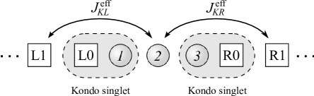
Figure 9: Schematic illustration for the $N_{c}=3$ chain with small inter-impurity coupling $J\lesssim T_{K,\alpha}^{1CK}$, as discussed in text.

II.2.1 Effective 2CK model for $N_{c}=3$

Before considering NRG calculations, we first derive the effective 2CK model for the simplest $N_{c}=3$ case; using perturbative techniques and scaling arguments, and exploiting the Wilson chain representationWilson (1975); Krishnamurthy et al. (1980); Bulla et al. (2008) (see Fig. 9) as natural within an RG framework.

The Wilson chain for lead $\alpha=L/R$ is definedWilson (1975); Krishnamurthy et al. (1980); Bulla et al. (2008) by dividing the band up into logarithmic intervals, $\{\pm D\Lambda^{-n}\}$ ($n=0,1,2,..$), and then discretizing it by retaining only the symmetric combination of states within each interval. This Hamiltonian is then tridiagonalized to obtain a linear chain form, with the impurity system coupled at one end.Wilson (1975); Krishnamurthy et al. (1980); Bulla et al. (2008) The $N_{c}=3$ Hamiltonian may thus be written in a dimensionless form $H_{N}=H_{0}+H_{1}$,

$$\begin{split}H_{0}&=\mathcal{J}_{KL}\hat{\textbf{S}}_{1}\cdot\hat{\textbf{s}}_{L0}+\mathcal{J}_{KR}\hat{\textbf{S}}_{3}\cdot\hat{\textbf{s}}_{R0}\\ H_{1}&=\mathcal{J}(\hat{\textbf{S}}_{1}\cdot\hat{\textbf{S}}_{2}+\hat{\textbf{S}}_{2}\cdot\hat{\textbf{S}}_{3})\\ &+\sum_{\alpha,\sigma}\sum_{n=0}^{N-1}t_{n}\left(f_{\alpha n\sigma}^{\dagger}f_{\alpha(n+1)\sigma}^{\phantom{\dagger}}+f_{\alpha(n+1)\sigma}^{\dagger}f_{\alpha n\sigma}^{\phantom{\dagger}}\right)\end{split}$$ (15)

where $\hat{\textbf{s}}_{\alpha 0}$ is given in Eq. 2 and the Wilson chain operators $f_{\alpha n\sigma}^{\dagger}$ are obtained recursively using the Lanczos algorithm.Wilson (1975) The rescaled dimensionless couplings are given by $\mathcal{J}_{K\alpha}=2\rho J_{K\alpha}/A_{N}$ and $\mathcal{J}=2\rho J/A_{N}$ (where $A_{N}=\tfrac{1}{2}(1+\Lambda^{-1})\Lambda^{-(N-1)/2}$). For a flat-band lead density of states, the tunnel-coupling between Wilson chain orbitals takes the formWilson (1975) $t_{n}=\Lambda^{(N-1)/2}\Lambda^{-n/2}\xi_{n}$, with the $\xi_{n}\equiv\xi_{n}(\Lambda)\sim\mathcal{O}(1)$. The full Hamiltonian is then recovered in the $N\rightarrow\infty$ limitWilson (1975); Krishnamurthy et al. (1980); Bulla et al. (2008) via $H={\text{lim}}_{N\rightarrow\infty}\left\{DA_{N}H_{N}\right\}$.

We consider first the limit of strong impurity-lead coupling, $\mathcal{J}_{K\alpha}\gg\max(\mathcal{J},t_{n})$; so that $H_{0}$ in Eq. 15 favours formation of a pair of singlet states between the terminal impurities and the ‘0’-orbital of their attached lead. The ground state of $H_{0}$ thus comprises a 1-‘L0’ singlet (we denote it by $|s;L\rangle$) and a 3-‘R1’ singlet (denoted $|s;R\rangle$), as shown schematically in Fig. 9.

$H_{1}$ now acts perturbatively, and we project onto the lowest state of $H_{0}$ using the unity operator for the reduced Hilbert space, $\hat{1}_{s}=|s;L\rangle|s;R\rangle\langle s;R|\langle s;L|$. An effective Hamiltonian may be obtained using the Brillouin-Wigner perturbation expansion,Ziman (1995) $H_{N}=E_{0}+H^{\text{eff}}_{\text{I}}+H^{\text{eff}}_{\text{II}}+H^{\text{eff}}_{\text{III}}+..$. Here, $E_{0}=\hat{1}_{s}H_{0}\hat{1}_{s}=-\tfrac{3}{4}(\mathcal{J}_{KL}+\mathcal{J}_{KR})$ is merely a constant shift in energy, while $H^{\text{eff}}_{\text{I}}=\hat{1}_{s}H_{1}\hat{1}_{s}\equiv\tilde{H}_{L}$ follows as

$$\tilde{H}_{L}=\sum_{\sigma,\alpha}\sum_{n=1}^{N-1}t_{n}\left(f_{\alpha n\sigma}^{\dagger}f_{\alpha(n+1)\sigma}^{\phantom{\dagger}}+f_{\alpha(n+1)\sigma}^{\dagger}f_{\alpha n\sigma}^{\phantom{\dagger}}\right)$$ (16)

and corresponds to a pair of free Wilson chains, with the ‘0’-orbital of each removed. The second-order term, $H^{\text{eff}}_{\text{II}}$ contributes only potential scatteringHewson (1993), here omitted for clarity. An effective coupling between impurity ‘2’ and the ‘L1’ and ‘R1’ orbitals is generated only to third-order in $H_{1}$, givenZiman (1995) by $H^{\text{eff}}_{\text{III}}=\hat{1}_{s}H_{1}(E_{0}-H_{0})^{-1}\hat{P}H_{1}(E_{0}-H_{0})^{-1}\hat{P}H_{1}\hat{1}_{s}$ with $\hat{P}=\hat{1}-\hat{1}_{s}$ a projector. Combining this with Eq. 15, a rather lengthy calculation yields

$$H^{\text{eff}}_{\text{III}}=\rho J_{KL}^{\text{eff}}\hat{\textbf{S}}_{2}\cdot\hat{\textbf{s}}_{L1}+\rho J_{KR}^{\text{eff}}\hat{\textbf{S}}_{2}\cdot\hat{\textbf{s}}_{R1}$$ (17)

(omitting RG irrelevant terms), with the effective coupling of impurity ‘2’ to the $\alpha=L$/$R$ lead given by

$$\rho J_{K\alpha}^{\text{eff}}=\left(\frac{20t_{0}^{2}\mathcal{J}}{9\mathcal{J}_{K\alpha}^{2}}\right)>0.$$ (18)

The effective model $H_{N}^{\text{eff}}=\tilde{H}_{L}+H^{\text{eff}}_{\text{III}}$, describes thereby the residual AF coupling between impurity ‘2’ and the ‘L1’ and ‘R1’ orbitals of a pair of leads (with impurities ‘1’ and ‘3’ and lead orbitals ‘L0’ and ‘R0’ removed); see Fig. 9. This is a model of 2CK form.

The above analysis presupposes the existence of the local singlet states $|s;L\rangle$ and $|s;R\rangle$. However, we note that for $J\lesssim T_{K,\alpha}^{1CK}$ (as given by Eq. 14), RG flow is expected near a Fermi liquid-type FP, comprising single-channel strong coupling states in each lead, with a free, disconnected local moment on impurity ‘2’ (and which ‘SC x SC x LM’ FP is of course stable only at the point $J=0$). Renormalization of the impurity-lead coupling $J_{K\alpha}\rightarrow\tilde{J}_{K\alpha}$ on successive reduction of the temperature/energy scale naturally results in incipient formation of Kondo singlets between each terminal impurity and its attached lead below $T\sim T_{K,\alpha}^{1CK}$ for the $\alpha=L/R$ channel, respectively. An effective 2CK model should then result via the mechanism described above, where the local singlet states $|s;L\rangle$ and $|s;R\rangle$ are now Kondo singlets.

The central question then is: how does Eq. 18 flow under renormalization? Specifically, what is the effective coupling $\rho\tilde{J}_{K\alpha}^{\text{eff}}$ for $T\sim T_{K,\alpha}^{1CK}$?

To answer this, recall first that the effective temperatureWilson (1975); Krishnamurthy et al. (1980); Bulla et al. (2008) within the RG framework is related to the iteration number/Wilson chain length, $N$, via $T\sim\Lambda^{-N/2}$. The operators for the Wilson chain orbitals also scale with $N$. In particular, operators for the ‘0’-orbital of the Wilson chain scale asWilson (1975); Krishnamurthy et al. (1980) $f_{\alpha 0\sigma}\sim\Lambda^{-N/4}$. Thus $\mathcal{J}_{K\alpha}\rightarrow\tilde{\mathcal{J}}_{K\alpha}\sim\Lambda^{-N/2}$, since the impurity-lead exchange coupling is associated with a pair of ‘0’-orbital fermionic operators. The key result is thus that the renormalized impurity-lead coupling $\tilde{\mathcal{J}}_{K\alpha}\sim T_{K,\alpha}^{1CK}$ for $T\sim T_{K,\alpha}^{1CK}$ — in accord with the physical expectation that disruption of the $\alpha=L/R$ Kondo singlet costs an energy $\mathcal{O}(T_{K,\alpha}^{1CK})$. By contrast, the coupling between the impurities, $\mathcal{J}$, is not associated with any chain operators, and hence does not get renormalized with $N$. Further, as pointed out in Ref. Chen and Jayaprakash, 1998, once the ‘0’-orbital of a Wilson chain has been frozen out (e.g. by formation of a Kondo singlet), the ‘1’-orbital operators then scale as $f_{\alpha 1\sigma}\sim\Lambda^{-N/4}$. Thus the renormalized tunnel-coupling $\tilde{t}_{0}\sim\Lambda^{-N/4}$, so that for $T\sim T_{K,\alpha}^{1CK}$, $\tilde{t}_{0}^{2}/\tilde{\mathcal{J}}_{K\alpha}$ remains $\mathcal{O}(1)$. From Eq. 18, the renormalized effective Kondo coupling at $T\sim T_{K,\alpha}^{1CK}$ can then be estimated to have the functional dependence $\rho\tilde{J}_{K\alpha}^{\text{eff}}\sim J/T_{K,\alpha}^{1CK}$.

For simplicity we focus now on the mirror symmetric case, where $J_{K\alpha}\equiv J_{K}$ and $T_{K,\alpha}^{1CK}\equiv T_{K}^{1CK}$, whence one has the effective low-energy Hamiltonian for $N_{c}=3$

$$H^{\text{eff}}_{N_{c}}=\tilde{H}_{L}+\rho\tilde{J}_{K,N_{c}}^{\text{eff}}\hat{\textbf{S}}\cdot(\hat{\textbf{s}}_{L1}+\hat{\textbf{s}}_{R1}),$$ (19)

with $\hat{\textbf{S}}\equiv\hat{\textbf{S}}_{2}$ and the effective coupling

$$\rho\tilde{J}_{K,N_{c}}^{\text{eff}}=\left(\frac{J}{T_{K}^{1CK}}\right)x(N_{c})$$ (20)

valid for $T\lesssim T_{K}^{1CK}$. Determination of the constant $x(N_{c})$ is obviously beyond the scope of this analysis, although it can be deduced directly from NRG calculations as demonstrated in the next section.

2CK physics is thus expected for $T\sim T_{K}^{2CK}$ ($\ll T_{K}^{1CK}$), as given from perturbative scalingNozières and Blandin (1980) by

$$T_{K}^{2CK}\sim T_{K}^{1CK}\rho\tilde{J}_{K,N_{c}}^{\text{eff}}\exp(-1/\rho\tilde{J}_{K,N_{c}}^{\text{eff}}),$$ (21)

where the physical origin of the prefactor $T_{K}^{1CK}$ is simply that the effective bandwidth of the problem is already reduced to $\sim T_{K}^{1CK}$ at the temperature $T\sim T_{K}^{1CK}$, below which the effective model, Eq. 19, is valid.

Figure 10: (A): $S_{\text{imp}}(T)/\ln(2)$ vs $T/D$ as the inter-impurity coupling is reduced, for the symmetric $N_{c}=3$ case ($\rho\delta_{K}=0$). Shown for fixed $\rho J_{K}=0.15$, varying $\rho J=\lambda(T_{K}^{1CK}/D)$, where $\lambda=10^{-n/10}$ and $n=0,5,7,9,11,13$ [lines (a)–(f)], with $T_{K}^{1CK}$ determined from a $J=0$ calculation. Behavior for $T\gg T_{K}^{2CK}$ is described by $S^{J=0}_{\text{imp}}(T)=\ln(2)+2S^{1CK}_{\text{imp}}(T)$ (diamonds), with $S^{1CK}_{\text{imp}}(T)$ for a single-channel Kondo model with the same $J_{K}$. (B): Comparison of behavior for $N_{c}=3,5,7$ (solid, dotted and dashed lines) with $J=\tfrac{1}{2}T_{K}^{1CK}$. (C): Results for $N_{c}=3,5,7$ (with $n=9$ and $11$): scaling collapse to the universal 2CK curve (circles) is seen in all cases.

II.2.2 NRG results for odd chains

The physical picture for the $N_{c}=3$ system is thus clear, and we now turn to NRG results for odd chains of length $N_{c}=3,5,7$ in the regime of weak coupling between the impurities. For accurate numerics, we found it necessary to retain $N_{s}=4000$, $6000$ and $12000$ states per iteration for $N_{c}=3$, $5$ and $7$, since higher-energy chain states remain important down to $T\sim J\lesssim T_{K}^{1CK}$.

Fig. 10(A) shows $S_{\text{imp}}(T)$ vs $T/D$ for the $N_{c}=3$ case discussed explicitly above; for a common $\rho J_{K}$ and with $\rho J=\lambda(T_{K}^{1CK}/D)$, where $\lambda=10^{-n/10}$ and $n=0,5,7,9,11,13$ [lines (a)–(f)]. $T_{K}^{1CK}$ was itself determined from a $J=0$ calculation which, modulo a free spin on impurity 2, is equivalent to two separate single-channel Kondo models with the same $J_{K}$. At high $T$, the trivial $S_{\text{imp}}=3\ln(2)$ behavior expected for three free spins-$\tfrac{1}{2}$ arises in all cases. Line (a) crosses directly to $S_{\text{imp}}=\tfrac{1}{2}\ln(2)$ on the scale $J=T_{K}^{1CK}\approx T_{K}^{2CK}$, characterizing flow to the 2CK FP. By contrast, lines (b)–(f) flow first to the SC x SC x LM FP ($S_{\text{imp}}=\ln(2)$). We also show for comparison $S^{J=0}_{\text{imp}}(T)=\ln(2)+2S^{1CK}_{\text{imp}}(T)$ (diamonds), where $S^{1CK}_{\text{imp}}(T)$ is the entropy of a single-channel Kondo modelHewson (1993) with the same Kondo coupling; $S^{J=0}_{\text{imp}}(T)$ thus describes the entire temperature-dependence of the entropy for $J=0$. Lines (c)–(f) follow this curve perfectly for $T\gg T_{K}^{2CK}$, as expected from the single-channel Kondo screening of impurities ‘1’ and ‘3’. An intermediate $S_{\text{imp}}=\ln(2)$ plateau is thus observed, the single-channel $T_{K}^{1CK}$ remaining constant while the two-channel scale $T_{K}^{2CK}$ diminishes rapidly as $J$ is decreased. RG flow thus persists in the vicinity of the SC x SC x LM FP over an extended $T$-range, but below $T\sim T_{K}^{2CK}$ all systems are described by the 2CK FP, with residual entropy $S_{\text{imp}}=\tfrac{1}{2}\ln(2)$.

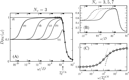
Figure 11: (A): Spectra $D\rho_{K}(\omega)$ vs $\omega/D$ as the inter-impurity coupling is reduced, for the symmetric $N_{c}=3$ case (with same parameters as Fig. 10). Behavior at $|\omega|\gg T_{K}^{2CK}$ is described by $D\rho_{K}^{1CK}(\omega)$ (diamond points) for a single-channel Kondo model. (B): Comparison of $N_{c}=3,5,7$ (solid, dotted, dashed lines) with $J=\tfrac{1}{2}T_{K}^{1CK}$. (C): Spectra vs $\omega/T_{K}^{2CK}$ for $N_{c}=3,5,7$ with $n=9$ and $11$: universal scaling collapse is seen. For $T_{K}^{2CK}\ll|\omega|\ll T_{K}^{1CK}$ the asymptotic behavior is $D\rho_{K}(\omega)=1-A/[\ln^{2}(|\omega|/T_{K}^{2CK})+B]$ (grey dashed line), while for $|\omega|\ll T_{K}^{2CK}$ NFL scaling is observed: $D\rho_{K}(\omega)=\tfrac{1}{2}[1+b(|\omega|/T_{K}^{2CK})^{1/2}]$ (grey dotted line). The entire curve is described by $D\rho_{K}(\omega)=1-D\rho_{K}^{2CK}(\omega)$ (circles), with $\rho_{K}^{2CK}(\omega)$ the scaling spectrum of the standard 2CK model.

We now comment on the generic behavior expected for impurity chains with $N_{c}>3$, which is a physically natural extension of the $N_{c}=3$ case above. Following the ‘removal’ of the terminal impurities through formation of single-channel Kondo singlets for $T\sim T_{K}^{1CK}$, the remaining odd $(N_{c}-2)$ impurities form a residual spin-$\tfrac{1}{2}$ on the scale $T\sim J$ ($\lesssim T_{K}^{1CK}$). This doublet state now feels an effective coupling to the two leads via the mechanism described in Sec. II.2.1, but with a further renormalization of the effective Kondo exchange, as expected from the discussion in Sec. II.1 in the regime of large inter-impurity coupling. Extension of the above analysis for $N_{c}=3$, which we do not give here, then leads us to expect (as tested below, Fig. 12) that the form Eq. 20 should hold for odd $N_{c}>3$, with ratios $x(N_{c}+2)/x(N_{c}=3)$ which are the same as those inferred from Table 1 but with two sites excluded from the spin-chain (reflecting quenching of the terminal spins ‘1’ and ‘$N_{c}$’ to form Kondo singlets); i.e. from Table 1 that $x(N_{c}=5)\approx\tfrac{2}{3}x(N_{c}=3)$ and $x(N_{c}=7)\approx 0.51x(N_{c}=3)$.

2CK physics is thus is expected for all odd chains in the small inter-impurity coupling regime below $T_{K}^{2CK}$, as given by Eqs. 21,20. This is confirmed in Fig. 10(B), where we consider chains of length $N_{c}=3,5,7$, taking $J=\tfrac{1}{2}T_{K}^{1CK}$ as an illustrative example. Again, at the highest temperatures $T\gg J$, one obtains $S_{\text{imp}}=N_{c}\ln(2)$. For sufficiently large separation between $T_{K}^{1CK}$ and $J$, one expects the entropy to drop first to $S_{\text{imp}}=(N_{c}-2)\ln(2)$ on the scale $T_{K}^{1CK}$ (due to single-channel Kondo quenchingHewson (1993) of the terminal impurities), followed by a further drop for $T\sim J$ to the LM value $S_{\text{imp}}=\ln(2)$; although in Fig. 10(B) $T_{K}^{1CK}$ and $J$ are comparable, so no distinct $(N_{c}-2)\ln(2)$ plateau arises. In all cases, however, $S_{\text{imp}}=\tfrac{1}{2}\ln(2)$ is seen below $T_{K}^{2CK}$, characteristic of flow to the stable 2CK FP;Cox and Zawadowski (1998) with scales $T_{K}^{2CK}$ that evidently diminish with increasing $N_{c}$, as expected qualitatively from the above discussion. Fig. 10(C) shows the scaling curve obtained when results are plotted vs $T/T_{K}^{2CK}$ (with $n=9,11$ chosen to ensure good scale separation between $T_{K}^{2CK}$ and $T_{K}^{1CK}$). The universal curve is precisely that of the standard 2CK model (circles).

Dynamics are now considered briefly, Fig. 11 (A) showing the $T=0$ $D\rho_{K}(\omega)$ for $N_{c}=3$ chains with the same parameters as in Fig. 10(A). All systems show RG flow in the vicinity of the Fermi liquid-type SC x SC x LM FP (reflecting single-channel Kondo screening of the terminal impurities), and hence an incipient single-channel Kondo resonanceHewson (1993) in each channel. For comparison, we show $D\rho^{1CK}_{K}(\omega)$ for a standard single-channel Kondo model with the same Kondo coupling (diamonds), which recovers perfectly the spectral behavior for $|\omega|\gg T_{K}^{2CK}$. In particular, for lines (d)–(f) in the range $T_{K}^{2CK}\ll|\omega|\ll T_{K}^{1CK}$, characteristic FL behaviorHewson (1993) $D\rho_{K}(\omega)=1-a(|\omega|/T_{K}^{1CK})^{2}$ arises, and thus the unitarity limit $D\rho_{K}(\omega)=1$ is reached in this intermediate energy window. For any finite $J$, $T_{K}^{2CK}$ is however always finite, so ultimately RG flow to the stable 2CK FP yields $D\rho_{K}(\omega)=\tfrac{1}{2}$ for $|\omega|\ll T_{K}^{2CK}$.

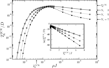
Figure 12: Evolution of the two-channel Kondo scale: $T_{K}^{2CK}/D$ vs $\rho J$ for symmetric chains of length $N_{c}=3,5,7$ (squares, diamonds and stars), and Kondo coupling $\rho J_{K}=0.15$ (with $\delta_{K}=0$). For large inter-impurity coupling, $T_{K}^{2CK}$ is given by Eqs. 7,8 (indicated by arrows). For each chain, the maximum value $T_{K}^{2CK}\approx T_{K}^{1CK}$ is obtained for $J\approx 10T_{K}^{1CK}$. For $J<T_{K}^{1CK}$, the Kondo scale diminishes rapidly; as seen also in the inset, where $\ln(T_{K}^{2CK})$ vs $T_{K}^{1CK}/J$ is shown, confirming Eqs. 20 and 21. The slopes yield $x(N_{c}=3)\approx 1/6$, $x(N_{c}=5)\approx 1/9$ and $x(N_{c}=7)\approx 1/12$.

Fig. 11(B) shows spectra for $N_{c}=3,5,7$ chains with common $J=\tfrac{1}{2}T_{K}^{1CK}$, as in Fig. 10(B). These display the same qualitative behavior as for $N_{c}=3$, with a single-channel Kondo resonance appearing at $|\omega|\sim T_{K}^{1CK}$, before crossing over to the 2CK FP for $|\omega|\sim T_{K}^{2CK}$. Since $T_{K}^{2CK}$ diminishes with increasing chain length, while $T_{K}^{1CK}$ remains fixed, apparent FL behavior consequently persists down to lower energies for the longer chains.

For $N_{c}=3,5,7$ chains with the same couplings as in Fig. 10(C), Fig. 11(C) shows the spectrum arising when results are shown vs $\omega/T_{K}^{2CK}$: collapse to a single universal scaling curve is seen clearly. One might naively expect to obtain the 2CK scaling spectrum here, since in this regime an effective 2CK model (Eq. 19) describes the system. However this model is only valid after the single-channel Kondo effect has already taken place in each lead, conferring a phase shift of $\pi/2$ to the conduction electrons.Hewson (1993) In consequence, the scaling spectrum in the small $J$ limit is $D\rho_{K}(\omega)=1-D\rho_{K}^{2CK}(\omega)$, with $D\rho_{K}^{2CK}(\omega)$ the scaling spectrum of the regular single-spin 2CK model. Comparison with the latter (circles) confirms this directly.

Finally, in Fig. 12 we analyze the variation of the two-channel Kondo scale as a function of the inter-impurity coupling strength, $\rho J$, and the chain length, $N_{c}$. The $T_{K}^{2CK}/D$ in the large-$J$ limit (indicated by arrows) are in accord with Eqs. 7,8. However, as $\rho J$ is decreased, $T_{K}^{2CK}$ first increases (reaching its maximum of $T_{K}^{2CK}\approx T_{K}^{1CK}$ for $J\approx 10T_{K}^{1CK}$ in each case), then diminishes very rapidly for $J\ll T_{K}^{1CK}$. The behavior for small inter-impurity coupling is seen most clearly in the inset, where $\ln(T_{K}^{2CK}/D)$ is shown vs $T_{K}^{1CK}/J$. The linear behavior confirms Eqs. 20,21, with the slopes yielding $x(N_{c}=3)\approx 1/6$, $x(N_{c}=5)\approx 1/9$ and $x(N_{c}=7)\approx 1/12$, as consistent with the expectation discussed above.

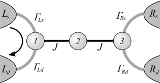
Figure 13: Schematic of the $N_{c}=3$ trimer with impurities ‘1’ and ‘3’ modelled as Anderson-like correlated levels, each tunnel-coupled to both source ($s$) and drain ($d$) leads, with hybridizations $\Gamma_{\alpha\gamma}$ (where $\alpha=L/R$ and $\gamma=s/d$). The impurities are exchange-coupled to eliminate $L\leftrightarrow R$ charge transfer processes that destroy 2CK physics, but conductance through impurity 1(3) in channel $\alpha=L(R)$ can be measured.

III Gate voltage effects and conductance

Having analyzed in detail the Heisenberg chain model, Eq. 1, we now consider a variant in which the terminal impurities are treated as correlated levels (dots), tunnel-coupled to their respective leads. Each lead $\alpha=L$ and $R$ can be ‘split’ into source ($s$) and drain ($d$), allowing the conductance through dot ‘1’ (or ‘$N_{c}$’) to be measured; see Fig.13. The Hamiltonian we study is $\mathcal{H}^{N_{c}}=\mathcal{H}_{L}+\mathcal{H}^{N_{c}}_{c}+\mathcal{H}^{N_{c}}_{\text{hyb}}$, where the four equivalent non-interacting leads are given by

$$\mathcal{H}_{L}=\sum_{\begin{subarray}{c}\alpha=L/R\\ \gamma=s/d\end{subarray}}\sum_{\textbf{k},\sigma}\epsilon^{\phantom{\dagger}}_{\textbf{k}}c^{\dagger}_{\alpha\gamma\textbf{k}\sigma}c^{\phantom{\dagger}}_{\alpha\gamma\textbf{k}\sigma},$$ (22)

and the impurity chain is described by

$$\begin{split}\mathcal{H}^{N_{c}}_{\text{c}}=&J\sum_{i=1}^{N_{c}-1}\hat{\textbf{S}}_{i}\cdot\hat{\textbf{S}}_{i+1}\\ &+U(\hat{n}_{1\uparrow}\hat{n}_{1\downarrow}+\hat{n}_{N_{c}\uparrow}\hat{n}_{N_{c}\downarrow})+\epsilon(\hat{n}_{1}+\hat{n}_{N_{c}}),\\ \end{split}$$ (23)

where $\hat{n}_{i}=\sum_{\sigma}\hat{n}^{\phantom{\dagger}}_{i\sigma}=\sum_{\sigma}d^{\dagger}_{i\sigma}d^{\phantom{\dagger}}_{i\sigma}$ is the number operator for dot $i=1$ or $N_{c}$, $\epsilon$ is its level energy and $U$ its Coulomb repulsion/charging energy. In a real quantum dot device, the level energy is proportional to the gate voltage, $\epsilon\propto V_{g}$. The leads and chain are coupled via

$$\mathcal{H}^{N_{c}}_{\text{hyb}}=\sum_{\begin{subarray}{c}\gamma=s/d\\ \textbf{k},\sigma\end{subarray}}\left(V^{\phantom{\dagger}}_{L\gamma}c_{L\gamma\textbf{k}\sigma}^{\dagger}d_{1\sigma}^{\phantom{\dagger}}+V^{\phantom{\dagger}}_{R\gamma}c_{R\gamma\textbf{k}\sigma}^{\dagger}d_{N_{c}\sigma}^{\phantom{\dagger}}+\text{H.c.}\right)$$ (24)

where $V_{\alpha\gamma}$ is the tunnel-coupling matrix element for the $\alpha=L/R$ and $\gamma=s/d$ lead. The hybridization strength follows as $\Gamma_{\alpha\gamma}=\pi\rho_{T}V^{2}_{\alpha\gamma}$ (with $\rho_{T}=N\rho$ the total lead density of states as before). Finally, a simple canonical transformation of the lead orbitals, via

$$\begin{split}c_{\alpha s\textbf{k}\sigma}=&a_{\alpha\textbf{k}\sigma}\cos(\theta_{\alpha})+\tilde{a}_{\alpha\textbf{k}\sigma}\sin(\theta_{\alpha})\\ c_{\alpha d\textbf{k}\sigma}=&a_{\alpha\textbf{k}\sigma}\sin(\theta_{\alpha})-\tilde{a}_{\alpha\textbf{k}\sigma}\cos(\theta_{\alpha})\end{split}$$ (25)

with $\tan(\theta_{\alpha})=V_{\alpha d}/V_{\alpha s}$, yields an effective two-channel model with

$$H_{L} =\sum_{\alpha,\textbf{k},\sigma}\epsilon^{\phantom{\dagger}}_{\textbf{k}}a^{\dagger}_{\alpha\textbf{k}\sigma}a^{\phantom{\dagger}}_{\alpha\textbf{k}\sigma}$$ (26a)

$$\mathcal{H}^{N_{c}}_{\text{hyb}} =\sum_{\textbf{k},\sigma}\left(V^{\phantom{\dagger}}_{L}a_{L\textbf{k}\sigma}^{\dagger}d_{1\sigma}^{\phantom{\dagger}}+V^{\phantom{\dagger}}_{R}a_{R\textbf{k}\sigma}^{\dagger}d_{N_{c}\sigma}^{\phantom{\dagger}}+\text{H.c.}\right)$$ (26b)

where $V_{\alpha}^{2}=V_{\alpha s}^{2}+V_{\alpha d}^{2}$; so that in particular for $V_{L}^{2}=V_{R}^{2}\equiv V^{2}$ (and hence $\Gamma_{L}=\Gamma_{R}\equiv\Gamma=\pi\rho_{T}V^{2}$) the model is mirror-symmetric. To investigate 2CK physics on the lowest energy scales, this is the situation now considered. We also focus on the simplest example of the $N_{c}=3$ trimer, variants of which have been studied recently in certain parameter regimes,Kuzmenko et al. (2006); Žitko et al. (2006); Mitchell et al. (2009); Numata et al. (2009); Žitko and Bonča (2007b); Žitko and Bonča (2008); Vernek et al. (2009); Mitchell and Logan (2010) including exchange-coupled chainŽitko and Bonča (2007b) and ringŽitko and Bonča (2008); Mitchell and Logan (2010) structures at half filling. As shown below, a physically intuitive perturbative treatment of the model for different fillings yield effective 2CK models – in spin and orbital sectors – from which the gate voltage-dependence of the 2CK scale can be identified.

III.1 Effective low-energy models for $N_{c}=3$

In the atomic limit ($V=0$) of the isolated $N_{c}=3$ trimer, the number of chain electrons jumps discontinuously between integer values $\mathcal{N}=n_{1}+n_{3}+1=1\rightarrow 5$ as the gate voltage $V_{g}\propto\epsilon$ is varied (recall that impurity ‘2’ is a strict spin-$\tfrac{1}{2}$). On tunnel-coupling to the leads, this Coulomb blockade (CB) staircase is naturally smoothed into a continuous crossover. Regimes of occupancy can still however be identified, and sufficiently deep within the CB valleys, $\mathcal{N}$ will be approximately integral. Here, a full $\mathcal{O}(V^{2})$ Schrieffer-Wolff (SW) transformationHewson (1993); Schrieffer and Wolff (1966) can be performed in the strongly correlated regime of interest $U\gg V$, perturbatively eliminating virtual excitations into high-energy manifolds with $(\mathcal{N}\pm 1)$ chain electrons.

In the atomic limit the ground state in any given $\mathcal{N}$-electron sector is a doublet, which we denote $|\mathcal{N};\pm\tfrac{1}{2}\rangle$. Projecting onto the reduced (chain) Hilbert space of this doublet using the unity operator

$$\hat{1}_{\mathcal{N}}=\sum_{\gamma=\pm\tfrac{1}{2}}|\mathcal{N};\gamma\rangle\langle\mathcal{N};\gamma|,$$ (27)

yields an effective model $\mathcal{H}_{\mathcal{N}}^{\text{eff}}=H_{L}+\mathcal{H}^{\text{eff}}_{\mathcal{N},\text{II}}$, where the leading $\mathcal{O}(V^{2})$ contribution arising from tunnel coupling to the leads (Eq. 26b with $V_{L}=V_{R}$ and $N_{c}=3$, denoted as $\mathcal{H}^{\prime}$) is given by the SW transformationHewson (1993); Schrieffer and Wolff (1966)

$$\mathcal{H}^{\text{eff}}_{\mathcal{N},\text{II}}=\hat{1}_{\mathcal{N}}\mathcal{H}^{\prime}(E_{0}-\mathcal{H}_{c}^{N_{c}=3})^{-1}\mathcal{H}^{\prime}\hat{1}_{\mathcal{N}}.$$ (28)

Here $E_{0}=\hat{1}_{\mathcal{N}}\mathcal{H}_{c}^{N_{c}=3}\hat{1}_{\mathcal{N}}$ is the energy of the ground chain doublet (and retardation has as usual been neglectedHewson (1993)).

In the following, we also exploit the particle-hole transformation

$$\begin{split}d_{i\sigma}^{\phantom{\dagger}}&\rightarrow d_{i\sigma}^{\dagger},\qquad~{}a_{\alpha\textbf{k}\sigma}^{\phantom{\dagger}}\rightarrow-a_{\alpha-\textbf{k}\sigma}^{\dagger}\\ \hat{S}_{2}^{\pm}&\rightarrow-\hat{S}_{2}^{\mp},\qquad~{}\hat{S}_{2}^{z}\rightarrow-\hat{S}_{2}^{z},\end{split}$$ (29)

which yields directly $\hat{\mathcal{N}}\rightarrow(6-\hat{\mathcal{N}})$. The full Hamiltonian (parameterized by $\mathcal{H}\equiv\mathcal{H}(\epsilon)$ for given $U$, $J$, $V$) transforms as $\mathcal{H}(\epsilon)\rightarrow\mathcal{H}(-\epsilon-U)+(2U-4\epsilon)$. In general, the physical behavior of $\mathcal{H}(\epsilon)$ and $\mathcal{H}(-\epsilon-U)$ is equivalent, since the constant shift $(2U-4\epsilon)$ is irrelevant in the calculation of observable quantities. Thus, the $\mathcal{N}=1\leftrightarrow 5$ and $\mathcal{N}=2\leftrightarrow 4$ sectors are related by the reflection about the particle-hole symmetric point $\epsilon=-\tfrac{1}{2}U$. Together with the singly-occupied $\mathcal{N}=3$-electron case, three distinct regions of electron filling must in consequence arise. We now considered them in turn.

III.1.1 $\mathcal{N}=3$ - electron regime

For $-(U+\tfrac{1}{4}J)<\epsilon<\tfrac{1}{4}J$, the atomic limit trimer ground state is a singly-occupied spin doubletMitchell and Logan (2010)

$$\begin{split}|\mathcal{N}=3;S^{z}\rangle=\tfrac{\sigma}{\sqrt{6}}\Big{[}\hat{S}_{2}^{\sigma}(d_{1\uparrow}^{\dagger}d_{3\downarrow}^{\dagger}-&d_{3\uparrow}^{\dagger}d_{1\downarrow}^{\dagger})\\ -&2\hat{S}_{2}^{-\sigma}d_{1\sigma}^{\dagger}d_{3\sigma}^{\dagger}\Big{]}|\text{vac}\rangle,\end{split}$$ (30)

where $S^{z}=\tfrac{\sigma}{2}$ with $\sigma=\pm$ for spins $\uparrow$$/$$\downarrow$, and $\hat{S}_{2}^{\sigma}\equiv\hat{S}_{2}^{\pm}$ is a spin raising/lowering operator. $|\text{vac}\rangle=\sum_{\sigma_{2}}|-;\sigma_{2};-\rangle$ defines the ‘vacuum’ state of the local (chain) Hilbert space, in which dots ‘1’ and ‘3’ are unoccupied, while ‘2’ carries a free spin-$\tfrac{1}{2}$.

Using Eq. 30 with Eqs. 27,28 leads eventually to the effective low energy model deep in the $\mathcal{N}=3$ CB valley:

$$\mathcal{H}^{\text{eff}}_{\mathcal{N}=3}=H_{L}+J_{K,\mathcal{N}=3}^{\text{eff}}\hat{\textbf{S}}\cdot(\hat{\textbf{s}}_{L0}+\hat{\textbf{s}}_{R0})$$ (31)

where we have omitted potential scattering contributions for clarity, and $\hat{\textbf{S}}$ is a spin-$\tfrac{1}{2}$ operator for the lowest chain doublet, defined by $\hat{S}^{z}=\sum_{S^{z}}|\mathcal{N}=3;S^{z}\rangle S^{z}\langle\mathcal{N}=3;S^{z}|$ and $\hat{S}^{\pm}=|\mathcal{N}=3;\pm\tfrac{1}{2}\rangle\langle\mathcal{N}=3;\mp\tfrac{1}{2}|$. Eq. 31 is of 2CK form, with effective Kondo coupling

$$\begin{split}\rho J_{K,\mathcal{N}=3}^{\text{eff}}=&\frac{4\Gamma}{6\pi}\bigg{\{}\frac{9}{J+4\epsilon+4U}+\frac{9}{J-4\epsilon}\\ &\quad-\frac{1}{5J+4\epsilon+4U}-\frac{1}{5J-4\epsilon}\bigg{\}},\end{split}$$ (32)

which is AF throughout the entire $\mathcal{N}\approx 3$ sector. In the particle-hole symmetric Kondo limit in particular ($\epsilon=-\tfrac{1}{2}U$), one obtains $\rho J_{K,\mathcal{N}=3}^{\text{eff}}=\tfrac{2}{3}\rho J_{K}$ to leading order in $1/U$ (with $\rho J_{K}=8\Gamma/(\pi U)$ the effective exchange coupling of a single Anderson impurityHewson (1993) tunnel-coupled to leads); which as such is consistent with Eq. 7 and Table 1 for the $N_{c}=3$ Heisenberg chain studied in Sec. II.1.

Two-channel Kondo physics thus arises in the $\mathcal{N}\approx 3$ regime, with $T_{K}^{2CK}$ in particular given from Eqs. 8, 32.

III.1.2 $\mathcal{N}=2,4$ - electron regime: orbital 2CK effect

As above, the $\mathcal{N}=2$ and $4$ electron regimes are related by the particle-hole transformation Eq. 29, so we consider explicitly only the $\mathcal{N}=4$ case. The $\mathcal{N}=4$ regime is the ground state of the free trimer over an $\epsilon$-interval of width $J/2$, specifically $-(U+\tfrac{3}{4}J)<\epsilon<-(U+\tfrac{1}{4}J)$. The ground state comprises a degenerate pair of spin singlets, since the spin-$\tfrac{1}{2}$ on impurity ‘2’ can form a local singlet with either ‘1’ or ‘3’ (the remaining site being doubly-occupied). Since the states are spin singlets, two-channel spin-Kondo physics will obviously not arise here.

The $\mathcal{N}=4$ states are however doubly degenerate, so may be associated with an orbital pseudospin ($\hat{\boldsymbol{\mathcal{T}}}$), and expressed as

$$\begin{split}|\mathcal{N}=4;\mathcal{T}^{z}\rangle=\tfrac{\sigma}{\sqrt{2}}\Big{[}\Big{(}\hat{S}_{2}^{-}&d_{(2+\sigma)\uparrow}^{\dagger}-\hat{S}_{2}^{+}d_{(2+\sigma)\downarrow}^{\dagger}\Big{)}\\ &d_{(2-\sigma)\uparrow}^{\dagger}d_{(2-\sigma)\downarrow}^{\dagger})\Big{]}|\text{vac}\rangle,\end{split}$$ (33)

with $\mathcal{T}^{z}=\tfrac{\sigma}{2}$ for $\sigma=\pm 1$. Projecting into this reduced Hilbert space using the $\mathcal{N}=4$ unity operator Eq. 27 with the SW transformation Eq. 28, yields an effective orbital 2CK model

$$\mathcal{H}^{\text{eff}}_{\mathcal{N}=4}=H_{L}+J_{K,\mathcal{N}=4}^{\text{eff}}\hat{\boldsymbol{\mathcal{T}}}\cdot(\hat{\boldsymbol{\tau}}_{0,\uparrow}+\hat{\boldsymbol{\tau}}_{0,\downarrow}),$$ (34)

with an effective exchange coupling

$$\begin{split}\rho J_{K,\mathcal{N}=4}^{\text{eff}}=\frac{\Gamma}{2\pi}\bigg{\{}&\frac{1}{\epsilon+U-\tfrac{3}{4}J}\\ &~{}~{}+\frac{2}{\epsilon+U+\tfrac{3}{4}J}-\frac{3}{\epsilon+U+\tfrac{1}{4}J}\bigg{\}}\end{split}$$ (35)

which is AF within the $\mathcal{N}\approx 4$ regime. The trimer orbital pseudospin $\hat{\boldsymbol{\mathcal{T}}}$ is a spin-$\tfrac{1}{2}$ operator defined by $\hat{\mathcal{T}}^{z}=\sum_{\mathcal{T}^{z}}|\mathcal{N}=4;\mathcal{T}^{z}\rangle\mathcal{T}^{z}\langle\mathcal{N}=4;\mathcal{T}^{z}|$ and $\hat{\mathcal{T}}^{\pm}=|\mathcal{N}=4;\pm\tfrac{1}{2}\rangle\langle\mathcal{N}=4;\mp\tfrac{1}{2}|$. Similarly, we may define a lead pseudospin $\hat{\boldsymbol{\tau}}_{0,\sigma}$ for each real spin $\sigma=\uparrow/\downarrow$ as $\hat{\tau}_{0,\sigma}^{z}=\tfrac{1}{2}(f_{L0\sigma}^{\dagger}f_{L0\sigma}^{\phantom{\dagger}}-f_{R0\sigma}^{\dagger}f_{R0\sigma}^{\phantom{\dagger}})$ and $\hat{\tau}_{0,\sigma}^{+}=f_{L0\sigma}^{\dagger}f_{R0\sigma}^{\phantom{\dagger}}$ (with $\hat{\tau}_{0,\sigma}^{-}=(\hat{\tau}_{0,\sigma}^{+})^{\dagger}$), where $f_{\alpha 0\sigma}^{\dagger}$ is given by Eq. 2b.

The important ‘pseudospin-flip’ processes embodied in Eq. 34 correspond physically to moving an electron of given real spin from one lead to the other, while simultaneously switching the trimer orbital participating in the local singlet, such that no net charge transfer occurs between leads. Real spin $\sigma=\uparrow/\downarrow$ here plays the role of the channel index, and as such orbital 2CK physics is expected below $T\sim T_{K}^{2CK}$, as given by Eq. 8 using the effective coupling Eq. 35.

III.1.3 $\mathcal{N}=1,5$ - electron regime

For $\epsilon<-(U+\tfrac{3}{4}J)$, the ground state in the atomic limit lies in the $\mathcal{N}=5$-electron regime. It is a spin doublet, comprising the free spin-$1/2$ on ‘impurity’ 2, with sites ‘1’ and ‘3’ each doubly occupied: $|\mathcal{N}=5;S^{z}\rangle=\hat{S}_{2}^{\sigma}d_{1\uparrow}^{\dagger}d_{1\downarrow}^{\dagger}d_{3\uparrow}^{\dagger}d_{3\downarrow}^{\dagger}|\text{vac}\rangle$. Virtual excitations to the $\mathcal{N}=4$-electron sectors are perturbatively eliminated to $\mathcal{O}(V^{2})$ by the SW transformation (Eq. 28), leading to

$$\mathcal{H}^{\text{eff}}_{\mathcal{N}=5}=H_{L}+J_{K,\mathcal{N}=5}^{\text{eff}}\hat{\textbf{S}}_{2}\cdot(\hat{\textbf{s}}_{L0}+\hat{\textbf{s}}_{R0}),$$ (36)

with effective coupling

$$\rho J_{K,\mathcal{N}=5}^{\text{eff}}=\frac{\Gamma}{\pi}\bigg{\{}\frac{1}{\epsilon+U-\tfrac{1}{4}J}-\frac{1}{\epsilon+U+\tfrac{3}{4}J}\bigg{\}}$$ (37)

which is AF throughout the $\mathcal{N}\approx 5$-electron regime. Two-channel spin-Kondo physics is thus again expected below $T\sim T_{K}^{2CK}$ (given via Eq. 8).

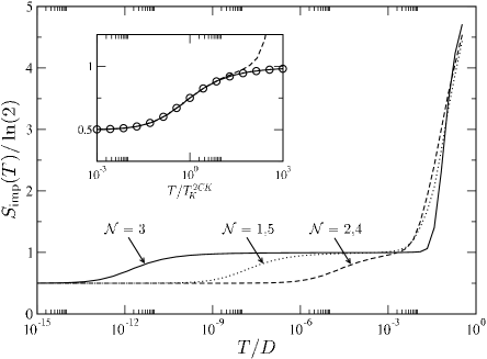
Figure 14: Entropy $S_{\text{imp}}(T)$ vs $T/D$ for a trimer with tunnel-coupled leads. Shown for $\rho J=0.075$, $U/\pi\Gamma=10$, $\Gamma/D=10^{-2}$, varying $\epsilon/\pi\Gamma=-5,-12.5,-14.5$ (solid, dashed and dotted lines), respectively representing systems ‘deep’ in the $\mathcal{N}=3,4,5$ CB valleys. Identical results are obtained for their particle-hole transformed counterparts. Inset: the low-temperature scaling behavior in terms of $T/T_{K}^{2CK}$, compared with the standard 2CK model (circles).

III.2 Thermodynamics and Scaling

The physical picture is clear: 2CK physics, whether of spin- or orbital-character, is expected when sufficiently deep in each region of electron filling. We confirm this directly using NRG for the full trimer model in Fig. 14, where the entropy $S_{\text{imp}}(T)/\ln(2)$ vs $T/D$ is shown for fixed representative $\rho J$, $U/\pi\Gamma$, and $\Gamma/D$, varying $\epsilon/\pi\Gamma$ for systems deep in the $\mathcal{N}=3,4,5$-electron CB valleys.

In each case, the high temperature $T>U$ behavior is simply that of two free orbitals and a free spin, giving $S_{\text{imp}}=5\ln(2)$. The LM FP is reached directly as $T$ is lowered, yielding $S_{\text{imp}}=\ln(2)$; flow to the 2CK FP with characteristicCox and Zawadowski (1998) $S_{\text{imp}}=\tfrac{1}{2}\ln(2)$ follows below $T\sim T_{K}^{2CK}$. Upon rescaling in terms of $T/T_{K}^{2CK}$ (see inset), the systems in each regime of filling collapse to the universal 2CK curve (circles), thus confirming the effective low-energy models Eqs. 31, 34 and 36.

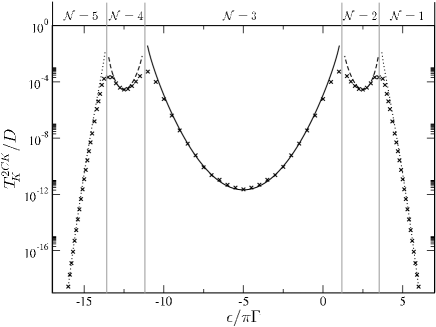
Figure 15: Evolution of the two-channel Kondo scale $T_{K}^{2CK}/D$ vs $\epsilon/\pi\Gamma$ for $\rho J=0.075$, $U/\pi\Gamma=10$ and $\Gamma/D=10^{-2}$. NRG results (points) are compared with Eq. 8 using effective Kondo couplings valid in the $\mathcal{N}=3$ regime (Eq. 32, solid line), $\mathcal{N}=2,4$ regimes (Eq. 35, dashed lines) and the $\mathcal{N}=1,5$ regimes (Eq. 37, dotted lines).

Fig. 15 shows the evolution of the 2CK scale as the level energy ($\epsilon\propto V_{g}$) is varied essentially continuously over a wide range of $\epsilon/\pi\Gamma$, for systems with the same $\rho J$, $U/\pi\Gamma$ and $\Gamma/D$ as in Fig. 14. NRG results (points) are compared with the perturbative result for $T_{K}^{2CK}$ given in Eq. 8, using the effective Kondo couplings valid in the $\mathcal{N}=3$ regime (Eq. 32), $\mathcal{N}=2,4$ regimes (Eq. 35) and the $\mathcal{N}=1,5$ regimes (Eq. 37). Throughout the majority of parameter space, the agreement is excellent; only at the boundary between regimes does the perturbative treatment (naturally) break down. Further, while the mechanism for overscreening changes from spin-2CK (odd-$\mathcal{N}$) to orbital-2CK (even-$\mathcal{N}$) across these boundaries, $T_{K}^{2CK}$ itself is found from NRG to vary smoothly; the 2CK FP remaining the stable FP in all cases (including for $\epsilon/\pi\Gamma<-14$ and $>+4$ in Fig. 15, where $T_{K}^{2CK}$ diminishes rapidly but nonetheless remains finite).

III.3 Single-particle dynamics and Conductance

We turn now to dynamics, focussing again on the spectrum $-\pi\rho_{T}\text{Im}[t_{L}(\omega)]\equiv\pi\Gamma D_{1}(\omega)$, where $D_{1}(\omega)=-\tfrac{1}{\pi}\text{Im}[G_{1}(\omega)]$ with $G_{1}$ the local retarded Green function for dot ‘1’. We obtain it through the Dyson equation,

$$[G_{1}(\omega)]^{-1}=[G_{1}^{0}(\omega)]^{-1}-\Sigma_{1}(\omega),$$ (38)

where $G_{1}^{0}(\omega)$ is the non-interacting propagator (obtained for $U=0=J$), and $\Sigma_{1}(\omega)=\Sigma_{1}^{R}(\omega)-i\Sigma_{1}^{I}(\omega)$ is the proper electron self-energy. The non-interacting $G_{1}^{0}(\omega)$ is simplyHewson (1993) $[G_{1}^{0}(\omega)]^{-1}=\omega^{+}-\epsilon-\Gamma(\omega)$ (with $\omega^{+}=\omega+i0^{+}$); where $\Gamma(\omega)=\Gamma^{R}(\omega)-i\Gamma^{I}(\omega)$, with $\Gamma^{I}(\omega)=\Gamma$ (=$\pi V^{2}\rho_{T}$) for all $|\omega|<D$ inside the band, and $\Gamma^{R}(\omega=0)=0$.

An expression for $\Sigma_{1}(\omega)$ is readily obtained using equation of motion methods,Hewson (1993); Zubarev (1960) and is given by

$$\begin{split}\Sigma_{1}(\omega)=[G_{1}(\omega)]^{-1}\bigg{\{}&U\langle\langle d^{\phantom{\dagger}}_{1\uparrow}\hat{n}^{\phantom{\dagger}}_{1\downarrow};d^{\dagger}_{1\uparrow}\rangle\rangle_{\omega}^{\phantom{\dagger}}\\ +&\tfrac{1}{2}J\langle\langle d^{\phantom{\dagger}}_{1\downarrow}\hat{S}_{2}^{-}+d^{\phantom{\dagger}}_{1\uparrow}\hat{S}_{2}^{z};d^{\dagger}_{1\uparrow}\rangle\rangle_{\omega}^{\phantom{\dagger}}\bigg{\}}\end{split}$$ (39)

where the local Green function itself is $G_{1}(\omega)=\langle\langle d^{\phantom{\dagger}}_{1\sigma};d^{\dagger}_{1\sigma}\rangle\rangle_{\omega}^{\phantom{\dagger}}$ (independent of spin $\sigma$ in the absence of a magnetic field, and with $G_{1}(\omega)=G_{3}(\omega)$ in the mirror-symmetric systems considered). The self-energy can be calculated directly within the density matrix formulation of NRGPeters et al. (2006); Weichselbaum and von Delft (2007); Bulla et al. (1998, 2008) via Eq. 39; with $G_{1}(\omega)$ then obtained from Eq. 38. In particular, the local propagator for $\omega=0$ may be expressed simply as $[G_{1}(0)]^{-1}=-\epsilon^{*}+i\Gamma^{*}$ in terms of the renormalized single-particle level $\epsilon^{*}$ and renormalized hybridization $\Gamma^{*}$, given by

$$\epsilon^{*} =\epsilon+\Sigma_{1}^{R}(0)$$ (40a)

$$\Gamma^{*} =\Gamma+\Sigma_{1}^{I}(0)$$ (40b)

in terms of the self-energy at $\omega=0$. The Fermi level value of the single-particle spectrum then follows as

$$\pi\Gamma D_{1}(\omega=0)~{}=~{}\frac{{}^{\phantom{*}}\Gamma^{\phantom{*}}}{{}^{\phantom{*}}\Gamma^{*}}~{}\frac{1}{1+(\epsilon^{*}/\Gamma^{*})^{2}}.$$ (41)

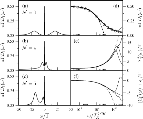
Figure 16: Left panels (a–c): $T=0$ single-particle spectrum $\pi\Gamma D_{1}(\omega)$ vs $\omega/\Gamma$. Shown for $\rho J=0.075$, $U/\pi\Gamma=10$, $\Gamma/D=10^{-2}$, with $\epsilon/\pi\Gamma=-5$ [$\mathcal{N}=3$, panel (a)], $-12.5$ [$\mathcal{N}\approx 4$, panel (b)] and $-14.5$ [$\mathcal{N}\approx 5$, panel (c)]. Panel (d): collapse to the universal 2CK scaling spectrum (circles). The scaling behavior of the proper self-energy, plotted as $\Sigma_{1}^{I}(\omega)/\Gamma$ and $[\Sigma_{1}^{R}(\omega)+\epsilon]/\Gamma$, is shown in panels (e) and (f). Asymptotic $|\omega|\ll T_{K}^{2CK}$ behavior described by $\pi\Gamma D_{1}(\omega)=\tfrac{1}{2}[1-b(|\omega|/T^{2CK}_{K})^{1/2}]$ (dashed line); $\Sigma^{I}_{1}(\omega)/\Gamma=1+2b(|\omega|/T_{K}^{2CK})^{1/2}$ (dotted); and $[\Sigma^{R}_{1}(\omega)+\epsilon]/\Gamma=-\text{sgn}(\omega)2b(|\omega|/T^{2CK}_{K})^{1/2}$ (dot-dashed).

NRG results are considered in Fig. 16, panels (a)–(c) showing $\pi\Gamma D_{1}(\omega)$ vs $\omega/\Gamma$ for fillings $\mathcal{N}=3,4,5$, with the same parameters as used in Fig. 14. First, we comment briefly on the high-energy ‘Hubbard satellites’ clearly visible in $D_{1}(\omega)$. As usual,Hewson (1993) these reflect simple one-electron addition ($\omega>0$) or subtraction ($\omega<0$) from the isolated chain $\mathcal{N}$-electron ground states. Their locations, broadened somewhat on coupling to the leads, are thus readily understood from the $V=0$ atomic limit ground states of Sec. III.1. Given their simplicity we do not comment further on them, save to note that in the $\mathcal{N}=3$ particle-hole symmetric example of panel (a), $D_{1}(\omega)=D_{1}(-\omega)$ as expected; and that for the $\mathcal{N}=5$ example in panel (c), high-energy features are naturally observed only for $\omega<0$, corresponding to excitations to $\mathcal{N}=4$-electron states.

The most important feature of $D_{1}(\omega)$ in Fig. 16 is of course the low-energy Kondo resonance, associated with RG flow in the vicinity of the stable 2CK FP. This is shown in panel (d) where spectra from the $\mathcal{N}=3,4,5$ regimes are again shown, but now rescaled in terms of $\omega/T_{K}^{2CK}$. Collapse to a single curve is seen, with the value at the Fermi level in particular pinned to $\pi\Gamma D_{1}(\omega=0)=\tfrac{1}{2}$, independent of $\epsilon$. The low-$\omega$ asymptotics of the scaling spectrum (dashed line) are found to be

$$\pi\Gamma D_{1}(\omega)~{}\overset{\tfrac{|\omega|}{T^{2CK}_{K}}\ll 1}{\sim}~{}\tfrac{1}{2}[1-b\left(|\omega|/T^{2CK}_{K}\right)^{1/2}],$$ (42)

as consistent with behavior near the 2CK FP discussed in connection with a variety of related two-channel models (see e.g. Refs. Affleck and Ludwig, 1993; Žitko and Bonča, 2007b; Johannesson et al., 2005; Bradley et al., 1999; Tóth and Zaránd, 2008; Mitchell and Logan, 2010; Anders, 2005). Indeed, comparison to the spectrum $D\rho_{K}(\omega)$ for the 2CK model shows perfect agreement in the low-energy scaling regime. This behavior is in striking contrast to that arisingHewson (1993) in a FL phase for $|\omega|\ll T_{K}$: $\pi\Gamma D(\omega)=\sin^{2}(\delta)-a_{1}(\omega/T_{K})-a_{2}(\omega/T_{K})^{2}$, describing the approach to the Fermi level value, which itself depends on the phase-shift, $\delta$. For the Anderson model,Hewson (1993) $\delta=\tfrac{\pi}{2}n_{\text{imp}}$ by the Friedel sum rule,Hewson (1993); Langreth (1966) with $n_{\text{imp}}$ the ‘excess’ charge in the system induced by addition of the impurity. Thus, $D(\omega=0)$ depends on the dot filling – and hence on the level energy $\epsilon$ – in a regular FL. The situation is clearly quite different in the stable NFL phase obtained for the chain models studied in the present work; and we shall consider the analogue of the Friedel sum rule in Sec. III.5 below.

Further insight is however gained from the electron self-energy itself, the imaginary and real parts of which are shown respectively in panels (e) and (f) of Fig. 16. To emphasise the low-energy scaling of interest, we show the results for $\mathcal{N}=3,4,5$ in terms of $\omega/T_{K}^{2CK}$. The common asymptotic form for $|\omega|\ll T_{K}^{2CK}$ is found to be

$$\Sigma^{I}_{1}(\omega)/\Gamma ~{}\sim~{}1+2b(|\omega|/T_{K}^{2CK})^{1/2},$$ (43a)

$$\Sigma^{R}_{1}(\omega)/\Gamma ~{}\sim~{}-\epsilon/\Gamma-\text{sgn}(\omega)2b(|\omega|/T^{2CK}_{K})^{1/2}$$ (43b)

(with $b\sim{\cal{O}}(1)$ precisely the same constant as in Eq. 42). At the Fermi level in particular, $\Sigma^{I}_{1}(\omega=0)=\Gamma$, in contrast to generic FL behavior $\Sigma^{I}(\omega=0)=0$. Indeed, extensive examination of NRG results over the entire parameter space confirms Eq. 43 generally – for any value of the bare level energy $\epsilon$, and for all interaction strengths $U/\Gamma$ and exchange couplings $\rho J>0$. The renormalized level energy and hybridization then follow from Eq. 40 as $\epsilon^{*}=0$ and $\Gamma^{*}=2\Gamma$. From Eq. 41, the spectrum at the Fermi level is in consequence pinned to a universal half-unitarity value, $\pi\Gamma D_{1}(\omega=0)=\tfrac{1}{2}$ for all underlying bare parameters, as illustrated in panel (d) of Fig. 16.

III.3.1 Conductance

To measure the differential conductance through dot ‘1’, a bias voltage $V_{sd}$ is applied across the $L$ source and drain leads, inducing a chemical potential difference $\mu_{s}-\mu_{d}=eV_{sd}$. The $L/R$ symmetry required to observe 2CK physics on the lowest energy scales also requires of course that the same bias be applied across the $R$ lead. Following Meir and Wingreen,Meir and Wingreen (1992) the zero-bias conductance through dot ‘1’ is given exactly by

$$G_{c}=\frac{2e^{2}}{h}G_{0}\int_{-\infty}^{\infty}\text{d}\omega(-)\frac{\partial f(\omega)}{\partial\omega}~{}\pi\Gamma D_{1}(\omega)$$ (44)

where $D_{1}(\omega)$ is the single-particle spectrum at equilibrium, $f(\omega)=[e^{\omega/T}+1]^{-1}$, and $\Gamma=\Gamma_{s}+\Gamma_{d}$ is the total hybridization as before. The dimensionless $G_{0}=4\Gamma_{s}\Gamma_{d}/(\Gamma_{s}+\Gamma_{d})^{2}$ embodies simply the relative coupling to source and drain leads; such that for $\Gamma_{s}=\Gamma_{d}$ $G_{0}=1$ is maximal, while in the extreme asymmetric limit $\Gamma_{s}\gg\Gamma_{d}$ (where the drain acts as a weak tunneling probe), $G_{0}\sim 4\Gamma_{d}/\Gamma_{s}\ll 1$.

For $T=0$, Eq. 44 reduces simply to

$$G_{c}^{0}=\frac{2e^{2}}{h}G_{0}\pi\Gamma D_{1}(\omega=0),$$ (45)

and Eq. 42 then gives a universal zero-bias conductance $G_{c}^{0}/G_{0}=e^{2}/h$ at $T=0$, obtained for any value of the gate voltage $V_{g}\propto\epsilon$. This result is thus consistent with that known for related models in the singly-occupied Kondo limit which demonstrate 2CK behavior (see e.g. Refs. Oreg and Goldhaber-Gordon, 2003; Potok et al., 2007; Pustilnik et al., 2004; Zaránd et al., 2006; Žitko and Bonča, 2007b; Tóth et al., 2007; Mitchell and Logan, 2010). For finite $T$, the Fermi level value of the spectrum has the same low-$T/T_{K}^{2CK}$ dependenceMitchell and Logan (2010) as the $T=0$ spectrum does of $\omega/T_{K}^{2CK}$ (Eq. 42), viz. $\pi\Gamma D_{1}(\omega=0;T)\sim\tfrac{1}{2}[1-b^{\prime}(T/T_{K}^{2CK})^{1/2}]$. Combined with Eq. 42, Eq. 44 is then readily shownMitchell and Logan (2010) to yield $G_{c}(T)/G_{0}\sim\tfrac{e^{2}}{h}[1-\gamma(T/T_{K}^{2CK})^{1/2}]$, with $\gamma=b^{\prime}+b\sqrt{\pi}\eta(\tfrac{1}{2})$ and $\sqrt{\pi}\eta(\tfrac{1}{2})\simeq 1.07$; which $T$-dependence is also known to arise for the single-spin 2CK model. Affleck and Ludwig (1993); Pustilnik et al. (2004); Tóth et al. (2007); Tóth and Zaránd (2008)

Calculating the conductance at finite bias is of course a different matter, and an exact (or even numerically exact) treatment of the underlying non-equilibrium physics is a formidable open problem. Here we merely make the simplifying approximation that the self-energy does not depend explicitly on the bias voltage,Anders et al. (2008) which leads to

$$G_{c}\simeq\frac{e^{2}}{h}G_{0}\int_{-\infty}^{\infty}\text{d}\omega\left(-\frac{\partial f_{s}(\omega)}{\partial\omega}-\frac{\partial f_{d}(\omega)}{\partial\omega}\right)\pi\Gamma D_{1}(\omega)$$ (46)

where $f_{\gamma}(\omega)=[e^{(\omega-\mu_{\gamma})/T}+1]^{-1}$ is the Fermi function for the $\gamma=s/d$ lead. While this approximation is exact both for $V_{sd}=0$, and for all $V_{sd}$ in the extreme asymmetric limit $\Gamma_{s}\gg\Gamma_{d}~{}$Pustilnik and Glazman (2004) (conductance measured with a ‘perfect STM’), in the standard case relevant to semiconductor quantum dot devices the leads are more symmetrically coupled. Here we consider a symmetric voltage split between the leads, $\mu_{s/d}=\pm\tfrac{1}{2}eV_{sd}$, for which Eq. 46 yields

$$G_{c}(V_{sd})\simeq\frac{e^{2}}{h}G_{0}\pi\Gamma\left[D_{1}(\omega=\tfrac{1}{2}eV_{sd})+D_{1}(\omega=-\tfrac{1}{2}eV_{sd})\right]$$ (47)

for $T=0$. This approximation thus allows us to work with single-particle spectra determined at equilibrium, obtained from a two-lead NRG calculationPeters et al. (2006); Weichselbaum and von Delft (2007); Bulla et al. (1998, 2008) as before.

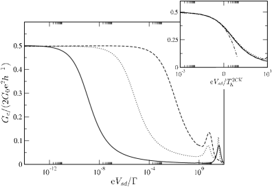
Figure 17: Conductance $G_{c}/(2G_{0}e^{2}h^{-1})$ vs $eV_{sd}/\Gamma$ for systems with same parameters as Figs. 14,16. Inset: scaling collapse to a universal curve with asymptotic $eV_{sd}\ll T_{K}^{2CK}$ behavior $G_{c}(V_{sd})=G_{0}e^{2}h^{-1}[1-b(eV_{sd}/T_{K}^{2CK})^{1/2}]$ (dot-dashed line).

Fig. 17 shows the resultant differential conductance $G_{c}/(2G_{0}e^{2}h^{-1})$ vs $eV_{sd}/\Gamma$, calculated using Eq. 47, for the same $\mathcal{N}=3,4,5$ systems as in Figs. 14 and 16. Since the conductance comprises a symmetrized combination of the total dot spectrum, similar features to that in Fig. 16 are naturally observed. Peaks at high bias originate from the Hubbard satellites, and correspond to simple single-electron sequential tunelling processes. Importantly, the Kondo resonance also of course shows up, with the zero-bias value of $G_{c}^{0}/G_{0}=e^{2}/h$ arising for $eV_{sd}\ll T_{K}^{2CK}$ in each case. Universal scaling of the conductance in terms of $eV_{sd}/T_{K}^{2CK}$ is also shown in the inset, demonstrating in particular the $eV_{sd}\ll T_{K}^{2CK}$ asymptotic form

$$G_{c}(V_{sd})~{}\overset{\tfrac{eV_{sd}}{T^{2CK}_{K}}\ll 1}{\sim}~{}\frac{e^{2}}{h}G_{0}[1-b(eV_{sd}/T_{K}^{2CK})^{1/2}],$$ (48)

which behavior is likewise knownOreg and Goldhaber-Gordon (2003); Potok et al. (2007); Pustilnik et al. (2004) in the NFL regime of the 2CK device constructed in Ref. Potok et al., 2007.

III.4 Phase shifts and the S-matrix

We now consider the leading low-$\omega$ behavior of the single-particle scattering S-matrix, $S(\omega)=e^{2i\delta(\omega)}$, and associated phase shift $\delta(\omega)=\delta_{R}(\omega)+i\delta_{I}(\omega)$. The S-matrix is given byLangreth (1966)

$$S(\omega)~{}=~{}1-2i\Gamma G_{1}(\omega),$$ (49a)

with $$\Gamma G_{1}(\omega) t_{L}(\omega)$$ related to the -matrix by

$$\pi\rho_{T}t_{L}(\omega)~{}=~{}\Gamma G_{1}(\omega)$$ (49b)

such that (as in Sec. III.3) $-\pi\rho_{T}\mathrm{Im}t_{L}(\omega)=\pi\Gamma D_{1}(\omega)$. It follows from Eq. 49a that

$$\pi\Gamma D_{1}(\omega)=\tfrac{1}{2}\left\{1-e^{-2\delta_{I}(\omega)}\cos(2\delta_{R}(\omega))\right\},$$ (50)

leading in particular to the limiting behavior:

$$\pi\Gamma D_{1}(\omega)=\begin{cases}\sin^{2}(\delta_{R}(\omega))&~{}~{}:\delta_{I}(\omega)\rightarrow 0\\ \tfrac{1}{2}&~{}~{}:\delta_{I}(\omega)\rightarrow\infty\end{cases}$$ (51)

To obtain $S(\omega)$ it is convenient to express the propagator as $G_{1}(\omega)~{}=~{}[A(\omega)+iB(\omega)]^{-1}$, where

$$A(\omega)~{}=~{}\omega-\epsilon-\Sigma_{1}^{R}(\omega),~{}~{}~{}B(\omega)~{}=~{}\Gamma+\Sigma_{1}^{I}(\omega)$$ (52)

such that $A(0)=-\epsilon^{*}$ and $B(0)=\Gamma^{*}$ by Eq. 40 (and for simplicity we take here the wide-band limit for the lead density of states, $\Gamma(\omega)=-i\Gamma$, which does not affect any of the following results). From Eq. 49a it follows that

$$e^{2i\delta(\omega)}~{}=~{}\frac{A(\omega)-iB^{\prime}(\omega)}{A(\omega)+iB(\omega)}$$ (53)

where

$$B^{\prime}(\omega)~{}=~{}\Gamma-\Sigma^{I}_{1}(\omega).$$ (54)

First consider the familiar situation that would arise if the system was a regular Fermi liquid, for which $\Sigma_{1}^{I}(\omega=0)=0$. In this case, $B(0)=B^{\prime}(0)$, and Eq. 53 yields $\delta(0)=\mathrm{arg}[G_{1}(0)]$. The S-matrix is then unitary at the Fermi level, $|S(0)|^{2}=1$; and, since $\delta_{I}(0)=0$, the Fermi level spectrum follows from Eq. 51 as $\pi\Gamma D_{1}(0)=\mathrm{sin}^{2}(\delta_{R}(0))$.

The situation is of course quite different for the present problem. The low-frequency behavior of the self-energy is given by Eqs. 43, and from which Eqs. 52-54 yield

$$e^{2i\delta(\omega)}~{}\sim~{}b\left(\frac{|\omega|}{T_{K}^{2CK}}\right)^{\frac{1}{2}}\left[1-i~{}\mathrm{sgn}(\omega)\right]$$ (55)

as the leading asymptotic form for $|\omega|/T_{K}^{2CK}\rightarrow 0$; i.e.

$$\delta_{R}(\omega)~{}\sim~{}\tfrac{1}{2}\mathrm{arctan}[-\mathrm{sgn}(\omega)]$$ (56a)

$$e^{-2\delta_{I}(\omega)}~{}\sim~{}\sqrt{2}b\left(\frac{|\omega|}{T_{K}^{2CK}}\right)^{\frac{1}{2}}.$$ (56b)

In evident contrast to a FL, the imaginary part of the phase shift thus diverges logarithmically as $\omega\rightarrow 0$,

$$\delta_{I}(\omega)~{}\sim~{}-\frac{1}{4}\ln(|\omega|/T_{K}^{2CK}),$$ (57)

the divergence itself reflecting (see Eq. 51) the pinning of the Fermi level spectrum to a half-unitary value (Sec. III.3). In consequence, the S-matrix vanishes at the Fermi level, $S(0)=0$, as known for the single spin-$\tfrac{1}{2}$ 2CK model. Maldacena and Ludwig (1997); Zaránd et al. (2004); Borda et al. (2007) This does not of course mean that an electron sent in to scatter off the dot is ‘absorbed’ (the conductance being generically non-zero), but rather that electrons scatter completely into collective excitations, characteristic of the NFL state. Maldacena and Ludwig (1997); Borda et al. (2007)

Notice also from Eq. 56a that the real part of the phase shift is discontinuous across the Fermi level, and that $\delta_{R}(\omega=0\pm)\neq\mathrm{arg}[G_{1}(0)]$ (again in contrast to a FL). $\mathrm{cos}(2\delta_{R}(0))=1/\sqrt{2}$ is however continuous across $\omega=0$ and, combined with Eq. 56b, Eq. 50 recovers precisely Eq. 42 for the low-$\omega$ asymptotics of $\pi\Gamma D_{1}(\omega)$.

III.5 Friedel-Luttinger sum rule

We now consider further implications of the pinning of the $T=0$ Fermi level spectrum, $\pi\Gamma D_{1}(0)=\tfrac{1}{2}$, regardless of bare model parameters and even when the dot occupancies change drastically on varying the bare level energy $\epsilon$. In particular, we obtain an analogue of the Friedel sum ruleHewson (1993); Langreth (1966) – a Friedel-Luttinger sum ruleLogan et al. (2009) – relating the Fermi level spectrum to the ‘excess’ charge induced by addition of the impurity chain,Hewson (1993) via the Luttinger integral.Luttinger (1960); Luttinger and Ward (1960)

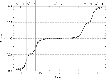
Figure 18: Luttinger integral $I_{L}/\pi$ vs level energy $\epsilon/\pi\Gamma$ for systems with $\rho J=0.075$, $U/\pi\Gamma=10$ and $\Gamma/D=10^{-2}$. Direct calculation via Eq. 63 shown as points, compared with Eq. 64 (line) using $n_{\text{imp}}$ determined from a standard thermodynamic NRG calculation.

To this end, consider first the excess charge $n_{\mathrm{imp}}$, defined as the difference in charge of the entire system with and without the trimeric impurity chain;Hewson (1993) and also $n_{\mathrm{imp}}^{\prime}$, defined correspondingly but with only the two terminal dots (‘1’ and ‘3’) of the chain removed. Since impurity ‘2’ is a strict spin, it follows trivially that $n_{\mathrm{imp}}=n_{\mathrm{imp}}^{\prime}+1$. Using e.g. equation of motion methods,Hewson (1993); Zubarev (1960) it is readily shown that

$$n_{\text{imp}}^{\prime}=-\frac{4}{\pi}\text{Im}\int_{-\infty}^{0}\text{d}\omega~{}G_{1}(\omega)\left[1-\frac{\partial\Gamma(\omega)}{\partial\omega}\right]$$ (58)

(noting that sites ‘1’ and ‘3’ are equivalent by symmetry). In practice, as expected physically, $n_{\mathrm{imp}}^{\prime}$ differs negligibly from the charge $2\langle\hat{n}_{1}\rangle$ on the terminal dots, to which it reduces precisely in the wide flat-band limit where $\Gamma(\omega)=-i\Gamma$ is constant.

Note next that Eq. 41 can be written as

$$\pi\Gamma D_{1}(\omega=0)=(\Gamma/\Gamma^{*})\sin^{2}(\theta)$$ (59)

with $\theta=\mathrm{arctan}(\Gamma^{*}/\epsilon^{*})$ ($\equiv\mathrm{arg}[G_{1}(0)]$). Equivalently, using $\mathrm{arg}[G_{1}(\omega=-\infty)]=0$,

$$\theta=\text{Im}\int_{-\infty}^{0}\text{d}\omega\frac{\partial}{\partial\omega}\ln G_{1}(\omega).$$ (60)

But from the definition of the propagator, $G_{1}(\omega)=[\omega^{+}-\epsilon-\Gamma(\omega)-\Sigma_{1}(\omega)]^{-1}$, it follows that

$$\frac{\partial}{\partial\omega}\ln G_{1}(\omega)=-G_{1}(\omega)\left[1-\frac{\partial\Gamma(\omega)}{\partial\omega}\right]+G_{1}(\omega)\frac{\partial\Sigma_{1}(\omega)}{\partial\omega}.$$ (61)

The Friedel-Luttinger sum rule then follows directly from Eq. 60 as

$$\theta=\frac{\pi}{4}n_{\text{imp}}^{\prime}+I_{L}$$ (62)

where the Luttinger integral Luttinger (1960); Luttinger and Ward (1960)

$$I_{L}=\text{Im}\int_{-\infty}^{0}\text{d}\omega~{}G_{1}(\omega)\frac{\partial\Sigma_{1}(\omega)}{\partial\omega}$$ (63)

involves integration over all energy scales.

Again consider briefly the situation that would arise if the system were a normal FL. In this case the Luttinger integral vanishesLuttinger (1960); Luttinger and Ward (1960) regardless of bare model parameters, and $\theta\equiv\delta_{R}(0)$ (as in Sec. III.4). Eq. 62 then reduces to a Friedel sum rule, Hewson (1993); Langreth (1966) relating the static phase shift to the excess charge.

The present problem is not of course a Fermi liquid, and $I_{L}$ does not vanish. The single-particle spectrum is however ubiquitously pinned at $\pi\Gamma D_{1}(\omega=0)=\tfrac{1}{2}$ (i.e. $\Gamma^{*}=2\Gamma$ and $\epsilon^{*}=0$), whence $\theta=\pi/2$ regardless of bare parameters.

Eq. 62 in this case thus becomes a sum rule relating the Luttinger integral to the excess charge:

$$I_{L}~{}=~{}\frac{\pi}{4}(2-n_{\text{imp}}^{\prime})~{}~{}=\frac{\pi}{4}(3-n_{\text{imp}})$$ (64)

Under the particle-hole transformation Eq. 29 it is easily shown that $n^{\prime}_{\mathrm{imp}}\rightarrow 4-n^{\prime}_{\mathrm{imp}}$ (or equivalently $n_{\mathrm{imp}}\rightarrow 6-n_{\mathrm{imp}}$). Hence $I_{L}\rightarrow-I_{L}$ under the transformation, and in particular vanishes at the particle-hole symmetric point $\epsilon=-U/2$ where $n_{\mathrm{imp}}=3$ identically.

The behavior of $n_{\mathrm{imp}}$ as e.g. the level energy $\epsilon$ is varied, is naturally a smoothed/continuous version of the Coulomb blockade staircase arising in the atomic limit (where on varying $\epsilon$ the total number of electrons in the free chain, ${\cal{N}}$, jumps discontinuously between integer values characteristic of each CB valley). $I_{L}$ itself will thus reflect that variation; and sufficiently deep in each CB valley, where $n_{\mathrm{imp}}$ ($\simeq{\cal{N}}$) is close to integral, each regime may be loosely associated with its own value of $I_{L}$.

The above discussion is exemplified clearly by Fig. 18, where the Luttinger integral $I_{L}/\pi$ is shown vs the level energy $\epsilon/\pi\Gamma$ for systems with common $U/\pi\Gamma=10$ and $\rho J=0.075$. The points correspond to direct calculation of $I_{L}$ via Eq. 63, using the full Green function and self-energy from NRG. The line is simply Eq. 64, using $n_{\text{imp}}$ as determined from a standard thermodynamic NRG calculation.Krishnamurthy et al. (1980) The agreement is excellent over the wide range of electron fillings shown, the overall form of the curve reflecting the smoothed CB staircase as anticipated above.

Our focus has been the $N_{c}=3$ trimer, but for longer (odd) chains one naturally expects the same 2CK physics to occur on low-energy scales. We have indeed confirmed this explicitly by NRG for the $N_{c}=5$ case. In particular, the single-particle spectrum of dot ‘1’ at the Fermi level is again always pinned to half-unitarity, $\pi\Gamma D_{1}(\omega=0)=\tfrac{1}{2}$ (whence the zero-bias conductance through a terminal dot remains $G_{c}/G_{0}=e^{2}/h$). The result $\theta=\pi/2$ thus holds generally, as does the Friedel-Luttinger sum rule Eq. 62, with $n_{\mathrm{imp}}^{\prime}$ now related to the total excess charge by $n_{\mathrm{imp}}=n_{\mathrm{imp}}^{\prime}+(N_{c}-2)$; and in consequence the general result for the Luttinger integral for odd chains follows:

$$I_{L}=~{}\frac{\pi}{4}(2-n_{\text{imp}}^{\prime})~{}~{}=\frac{\pi}{4}(N_{c}-n_{\text{imp}})$$ (65)

IV Concluding Remarks: Real Quantum Dot systems

The exchange-coupled impurity chains studied in this paper may be considered as approximate low-energy models of quantum dot devices. In real systems, however, the dots are mutually tunnel-coupled rather than pure exchange-coupled; the 2CK fixed point is rendered unstable by the inter-lead charge transfer that results, and the system crosses over to FL behavior on a low-energy scale $T\lesssim T_{\text{FL}}$. Experimental access to 2CK physics must thus contend with both channel anisotropy (as studied in Sec. II), and charge transfer terms. On the level of a toy model calculation, we now consider briefly the generic behavior arising when the latter perturbation is included, considering explicitly the $L/R$ mirror symmetric case (although the analysis is readily extended to include explicit channel anisotropy).

To motivate this, recall that a single ($N_{c}=1$) one-level quantum dot tunnel-coupled to two metallic leads does not of course exhibit 2CK physics.Pustilnik and Glazman (2004); Goldhaber-Gordon et al. (1998); Cronenwett et al. (1998) This follows from the Anderson Hamiltonian itself, $H_{\text{And}}=H_{\text{dot}}+\sum_{\alpha=L/R}[H^{\alpha}_{L}+H^{\alpha}_{\text{hyb}}]$; where $H_{\text{dot}}=\epsilon(\hat{n}_{d\uparrow}+\hat{n}_{d\downarrow})+U\hat{n}_{d\uparrow}\hat{n}_{d\downarrow}$, $H^{\alpha}_{L}=\sum_{\textbf{k},\sigma}\epsilon_{\textbf{k}}a_{\alpha\textbf{k}\sigma}^{\dagger}a_{\alpha\textbf{k}\sigma}^{\phantom{\dagger}}$ and $H^{\alpha}_{\text{hyb}}=V\sum_{\textbf{k},\sigma}(a_{\alpha\textbf{k}\sigma}^{\dagger}d^{\phantom{\dagger}}_{\sigma}+\text{H.c.})$. Transforming canonically to even ($e$) and odd ($o$) lead orbitals

$$\begin{split}a_{e\textbf{k}\sigma}=&\tfrac{1}{\sqrt{2}}\left(a_{L\textbf{k}\sigma}+a_{R\textbf{k}\sigma}\right)\\ a_{o\textbf{k}\sigma}=&\tfrac{1}{\sqrt{2}}\left(a_{L\textbf{k}\sigma}-a_{R\textbf{k}\sigma}\right),\end{split}$$ (66)

$H_{\text{And}}$ is equivalent to $H_{\text{And}}=H_{\text{dot}}+H^{e}_{L}+\sqrt{2}H^{e}_{\text{hyb}}$, in which the dot couples solely to the $e$-lead; exhibiting as such single-channel physics only.

In the singly-occupied dot regime, a low-energy spin-$\tfrac{1}{2}$ Kondo model follows from a SW transformationHewson (1993); Schrieffer and Wolff (1966) of $H_{\text{And}}$, leading simply to $H_{\text{SW}}=H_{L}^{L}+H_{L}^{R}+H_{K}$ with

$$H_{K}=J_{K}\hat{\textbf{S}}\cdot(\hat{\textbf{s}}_{L0}+\hat{\textbf{s}}_{R0})+J_{LR}\hat{\textbf{S}}\cdot\hat{\textbf{s}}_{LR0}$$ (67)

(potential scattering is ignored); where $\hat{\textbf{s}}_{\alpha 0}$ is given by Eq. 2, and $\hat{\textbf{s}}_{LR0}$ is defined as

$$\hat{\textbf{s}}_{LR0}=\sum_{\sigma,\sigma^{\prime},\alpha}f^{\dagger}_{\alpha 0\sigma}\boldsymbol{\sigma}_{\sigma\sigma^{\prime}}f^{\phantom{\dagger}}_{\bar{\alpha}0\sigma^{\prime}}$$ (68)

with $\bar{\alpha}=R,L$ for $\alpha=L,R$. Eq. 67 consists formally of a symmetric 2CK model – the first term – together with a term $\hat{\textbf{S}}\cdot\hat{\textbf{s}}_{LR0}$ which transfers (cotunnels) charge between the leads. In fact, applying the transformation Eq. 66 yields $H_{\text{SW}}=H_{L}^{e}+H_{L}^{o}+H_{K}$ with

$$H_{K}=J_{K}\hat{\textbf{S}}\cdot(\hat{\textbf{s}}_{e0}+\hat{\textbf{s}}_{o0})+J_{LR}\hat{\textbf{S}}\cdot(\hat{\textbf{s}}_{e0}-\hat{\textbf{s}}_{o0}),$$ (69)

where $\hat{\textbf{s}}_{e0}$ and $\hat{\textbf{s}}_{o0}$ are $e/o$ lead spin densities; a model that is generically of channel-asymmetric 2CK form. But for the single-dot Anderson model itself the couplings are necessarily equal, $J_{LR}=J_{K}$. In this case the dot is exchange-coupled solely to the even lead, and Eq. 69 reduces as it must to a single-channel Kondo model with Kondo coupling $2J_{K}$.

In systems comprising several tunnel-coupled quantum dots, however, cotunneling charge-transfer can be effectively suppressed,Zaránd et al. (2006) with $J_{LR}\ll J_{K}$ expected for longer chains (a simple estimate yielding $J_{LR}/J_{K}\sim[t/U]^{N_{c}-1}$ with $t$ the inter-dot tunnel coupling). Here we simply regard Eq. 67, with $J_{LR}\neq J_{K}$, as an effective toy model to mimic such effects in odd-$N_{c}$ dot chains (with $\hat{\textbf{S}}$ representing the lowest chain doublet). From Eq. 69 it is clear that the resultant low-energy/$T$ physics is then that of the channel-asymmetric 2CK model.Nozières and Blandin (1980); Cox and Zawadowski (1998); Sacramento and Schlottmann (1989); Andrei and Jerez (1995); Affleck et al. (1992) The 2CK FP is thus rendered unstable by the perturbation $J_{LR}$, any nascent 2CK state forming at $T_{K}^{2CK}$ being destroyed below the FL crossover scale $T_{\text{FL}}$; although inclusion of the $J_{LR}$ term should not obscure the 2CK physics for $T\gg T_{\text{FL}}$, provided $J_{LR}$ itself is sufficiently small. Note also that any direct inter-lead tunneling terms of the type $\sum_{\mathbf{k},\mathbf{k}^{\prime}}(a_{L\textbf{k}\sigma}^{\dagger}a^{\phantom{\dagger}}_{R\textbf{k}^{\prime}\sigma}+\text{H.c.})$ – as opposed to cotunneling which intrinsically proceeds via the dot spin – are equivalent (through the transformation Eq. 66) to simple potential scattering in the even and odd channels. This does not destabilise the 2CK FP,Affleck and Ludwig (1990) for which reason we do not include such terms here.

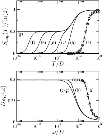
Figure 19: Upper panel: entropy $S_{\text{imp}}(T)$ vs $T/D$ for a single-spin 2CK model with explicit left/right lead charge transfer (see Eq. 67). Shown for fixed $\rho J_{K}=10^{-1}$, varying $\rho J_{LR}=10^{-1},10^{-2},10^{-3},10^{-4},10^{-5},10^{-6}$ [lines (a)–(f)], successively approaching the pure 2CK limit with $\rho J_{LR}=0$, line (g). Lower panel: $T=0$ spectra $D\rho_{K}(\omega)$ vs $\omega/D$ for the same systems. $S_{\text{imp}}^{1CK}(T)$ and $\tfrac{1}{2}D\rho_{K}^{1CK}(\omega)$ for a 1CK model with $\rho J_{K}=0.2$ (circles) are also shown for comparison.

The above scenario is explored in Fig. 19, where NRG results for Eq. 67 are shown. We fix $\rho J_{K}=10^{-1}$, and vary the cotunneling term $\rho J_{LR}=10^{-1},10^{-2},10^{-3},10^{-4},10^{-5}$ and $10^{-6}$ [lines (a)–(f)], approaching the pure 2CK limit $J_{LR}=0$ [line (g)]. The top panel shows the entropy $S_{\text{imp}}(T)/\ln(2)$ vs $T/D$, from which the behavior associated with the channel-asymmetric 2CK modelNozières and Blandin (1980); Cox and Zawadowski (1998); Sacramento and Schlottmann (1989); Andrei and Jerez (1995); Affleck et al. (1992) is seen to arise, as expected from Eq. 69. In the extreme case $J_{K}=J_{LR}$ [line (a)], the odd channel is completely decoupled, no 2CK physics occurs, and the behavior is that of a single-channel Kondo model (circles); the impurity entropy being completely quenched below $T\sim T_{K}^{1CK}$ (cf. Eq. 14). For smaller $J_{LR}\lesssim T_{K}^{1CK}$ however, the 2CK scale $T_{K}^{2CK}$ emerges (cf. Eq. 8), below which temperature a characteristic $S_{\text{imp}}=\tfrac{1}{2}\ln(2)$ plateau occurs [lines (d)–(g)]. Flow to the FL FP below $T\sim T_{\text{FL}}$, for all systems with $J_{LR}\neq 0$, is then manifest in the final drop to $S_{\text{imp}}=0$; the FL crossover scale $T_{\text{FL}}$ being found to vanish as

$$T_{\text{FL}}~{}\overset{J_{LR}\rightarrow 0^{\pm}}{\sim}~{}{\cal{A}}|J_{LR}|^{\nu}~{}~{}~{}~{}~{}~{}:\nu=2$$ (70)

with exponent $\nu=2$, just as expected from mapping to the channel-asymmetric 2CK model, Eq. 69.

We turn now to the $T=0$ spectra $D\rho_{K}(\omega)\equiv D\rho_{K,\alpha}(\omega)=-\pi\rho_{T}\text{Im}[t_{\alpha}(\omega)]$ for lead $\alpha=L$ or $R$ (the two being equivalent by mirror symmetry), shown in the lower panel of Fig. 19. The spectral behavior is rather different from what might naively be expected from the entropy, since no low-energy $T_{\text{FL}}$ scale is apparent (compare e.g. to the channel-asymmetric 2CK models studied in Fig. 7). This however reflects the fact that the model Eq. 67 is channel-asymmetric 2CK in the $e/o$ basis (Eq. 69), rather than the $L/R$ basis; and is readily understood using the transformation Eq. 66, from which one obtains $D\rho_{K,\alpha}(\omega)=\tfrac{1}{2}[D\rho_{K,e}(\omega)+D\rho_{K,o}(\omega)]$ in terms of the spectra for $e/o$ channels. For $J_{K}=J_{LR}$ [line (a)], the odd channel is decoupled in Eq. 69, so $D\rho_{K,\alpha}(\omega)=\tfrac{1}{2}D\rho_{K,e}(\omega)\equiv\tfrac{1}{2}D\rho_{K}^{1CK}(\omega)$, where $D\rho_{K}^{1CK}(\omega)$ is the spectrum for a 1CK model with Kondo coupling $2J_{K}$ (as confirmed explicitly (circles) in the lower panel of Fig. 19).

However, for lines (c)–(f) (corresponding to $J_{LR}\ll T_{K}^{1CK}$), the spectra are indistinguishable from the pure 2CK spectrum, line (g), over the entire range of frequencies. For $T_{\text{FL}}\ll|\omega|\ll T_{K}^{2CK}$, RG flow in the vicinity of the 2CK FP naturally results in the universal behavior $D\rho_{K,e}(\omega)=D\rho_{K,o}(\omega)=\tfrac{1}{2}[1-b(|\omega|/T_{K}^{2CK})^{1/2}]$, as expected for a 2CK model with small even/odd channel asymmetry (see Fig. 7). Consequently $D\rho_{K}(\omega)$ shows the same behavior. For $|\omega|\ll T_{\text{FL}}$ by contrast, the spectrum for the more strongly coupled $e$-channel has the asymptotic form $D\rho_{K,e}(\omega)=1-d(|\omega|/T_{\text{FL}})^{2}$ while the weakly coupled $o$-channel is described by $D\rho_{K,o}(\omega)=d(|\omega|/T_{\text{FL}})^{2}$ (see Fig. 7 and discussion thereof). Indeed, we found in Sec. II.1 that the entire universal crossover to the Fermi liquid FP for the strongly coupled lead is related to that of the weakly coupled lead by $D\rho_{K,e}(\omega)=1-D\rho_{K,o}(\omega)$. Thus, $D\rho_{K}(\omega)=\tfrac{1}{2}$ arises for all $|\omega|\ll T_{K}^{2CK}$, as indeed found. As such, the spectrum $D\rho_{K}(\omega)$ is effectively ‘blind’ to the Fermi liquid crossover induced by small finite $J_{LR}$: the 2CK FP appears to be stable on the lowest energy scales – although from e.g. the entropy we know that this is not the case. Ironically, then, experiments that probe the t-matrix (such as measurement of the zero-bias conductance across dot ‘1’) will always appear to yield 2CK physics, provided $J_{LR}\lesssim T_{K}^{1CK}$.