The relationship between a topological Yang-Mills field and a magnetic monopole

Abstract

We show that a Jackiw-Nohl-Rebbi solution, as the most general two-instanton, generates a circular loop of magnetic monopole in four-dimensional Euclidean $SU(2)$ Yang-Mills theory.

1 Introduction

It is believed that a promising mechanism for quark confinement is the dual superconductivity proposed in dualsuper ; Polyakov77 . In this mechanism, condensation of magnetic monopoles causes confinement. Therefore, it must be shown that magnetic monopoles to be condensed exist in Yang-Mills theory. In the lattice simulation SKKISF09 , magnetic monopoles are exist in Yang-Mills theory and magnetic monopole currents form loops. In regard to this result, we can ask the following question. Which configuration of the Yang-Mills field can be the source for such magnetic monopoles? The simplest configuration examined first was the one-instanton configuration, which is a solution of the self-dual equation ${}^{\ast}F=\pm F$ and has a unit instanton charge $|Q_{p}|=1$. However, it has been confirmed in KFSS08 ; CG95 ; BOT97 that magnetic monopole loops are not generated from the one-instanton solution.

In this study, we examine the Jackiw-Nohl-Rebbi (JNR) two-instanton solution. We demonstrate in a numerical way that a circular loop is generated from the JNR solution. We construct the magnetic monopole current based on the nonlinear change of variables (NLCV) and the reduction condition KSM08 ; KSSMKI08 . The NLCV is a gauge-invariant extension of the Abelian projection invented by ’t Hooft tHooft81 and enables one to extract magnetic monopoles from the original Yang-Mills theory without breaking the gauge symmetry.

2 The difinition of magnetic monopole

We summarize the method in a continuum $SU(2)$ Yang-Mills theory. We introduce a color field ${\bf n}(x)$ with a unit length: ${\bf n}(x)=n^{A}(x)T^{A},n^{A}(x)n^{A}(x)=1,(T^{A}:=\sigma_{A}/2)$, where $\sigma_{A}\ (A=1,2,3)$ are Pauli matrices. The color field is determined by imposing the reduction condition. It is given by minimizing the functional

$$F_{\mbox{\footnotesize red}}:=\int d^{4}x\frac{1}{2}\mbox{tr}[\{D_{\mu}[{\bf A}]{\bf n}(x)\}^{2}].$$ (1)

The local minima are given by the reduction differential equation (RDE) KFSS08 :

$$-D_{\mu}[{\bf A}]D_{\mu}[{\bf A}]{\bf n}(x)=\lambda(x){\bf n}(x).$$ (2)

Once the RDE is solved for a given ${\bf A}_{\mu}$, we can obtain the gauge invariant magnetic monopole current $k^{\mu}$ by the following equations (NLCV).

$${\bf V}_{\mu}(x):=2\mbox{tr}\left({\bf n}(x){\bf A}_{\mu}(x)\right){\bf n}(x)-ig^{-1}\left[\partial_{\mu}{\bf n}(x),{\bf n}(x)\right],$$ (3)

$${\bf F}_{\mu\nu}[{\bf V}]=\partial_{\mu}{\bf V}_{\nu}-\partial_{\nu}{\bf V}_{\mu}-ig\left[{\bf V}_{\mu},{\bf V}_{\nu}\right],$$ (4)

$$k^{\mu}(x):=\partial_{\nu}\!\,^{\ast}G^{\mu\nu}(x)=\epsilon^{\mu\nu\rho\sigma}\partial_{\nu}G_{\rho\sigma}(x)/2,\quad G_{\mu\nu}(x)=2\mbox{tr}({\bf n}{\bf F}_{\mu\nu}[{\bf V}]).$$ (5)

We carry out this procedure numerically. We use the lattice regularization and a lattice version of the NLCV SKS10 for numerical calculation. In solving the RDE numerically, we must fix the asymptotic behavior of ${\bf n}$. We recall that the instanton configuration approaches a pure gauge at infinity: $g{\bf A}_{\mu}(x)\rightarrow ih^{\dagger}(x)\partial_{\mu}h(x)+O(|x|^{-2}).$ Then, ${\bf n}(x)$ as a solution of the reduction condition is supposed to behave asymptotically ${\bf n}(x)\rightarrow h^{\dagger}(x)T_{3}h(x)+O(|x|^{-\alpha}),$ for a certain value of $\alpha>0$. Actually, since we solve the RDE on a finite volume $V$, we adopt a boundary condition as ${\bf n}^{{\mbox{\footnotesize bound}}}(x)=h^{\dagger}(x)T_{3}h(x),\ x\in\partial V$.

3 result

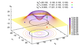
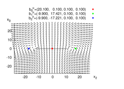
Figure 1: (Left panel) The JNR two-instanton and the associated circular loop of the non-zero magnetic monopole current $k_{\mu}(x)$. The JNR two-instanton is defined by fixing three scales $\rho_{0}=\rho_{1}=\rho_{2}=3$ and three pole positions $b_{0}^{\mu},b_{1}^{\mu},b_{2}^{\mu}$ which are arranged to be three vertices of an equilateral triangle. The grid shows an instanton charge density $D(x)$ on $x_{1}$-$x_{2}$ ($x_{3}=x_{4}=0$) plane. The black (thick) line on the base shows the magnetic monopole loop projected on $x_{1}$-$x_{2}$ plane, while colored (thin) lines on the base show the contour plot for the equi-$D(x)$ lines. (Right panel) The configuration of the color field ${\bf n}=(n_{1},n_{2},n_{3})$ and a circular loop of the magnetic monopole current $k_{\mu}(x)$ obtained from the JNR two-instanton, viewed in the $x_{2}$-$x_{3}$ ($x_{1}=x_{4}=0$) plane which is off three poles. The magnetic monopole current and the three poles of the JNR solution are projected on the same plane. Here the $SU(2)$ color field $(n_{1},n_{2},n_{3})$ is identified with a unit vector in the three-dimensional space $(x_{1},x_{2},x_{3})$.

The explicit form of the JNR two-instanton solution is

$$g{\bf A}_{\mu}(x)=T^{A}\eta_{\mu\nu}^{A(-)}\phi_{\rm JNR}^{-1}\sum_{r=0}^{2}\frac{2\rho_{r}^{2}\left(x^{\nu}-b^{\nu}_{r}\right)}{(|x-b_{r}|^{2})^{2}},\ \phi_{\rm JNR}:=\sum_{r=0}^{2}\frac{\rho_{r}^{2}}{|x-b_{r}|^{2}},$$ (6)

where $|x|^{2}=x_{\mu}x^{\mu}$. The JNR two-instanton is specified by three pole positions $(b_{0}^{1},b_{0}^{2},b_{0}^{3},b_{0}^{4})$, $(b_{1}^{1},b_{1}^{2},b_{1}^{3},b_{1}^{4})$, $(b_{2}^{1},b_{2}^{2},b_{2}^{3},b_{2}^{4})$ and three scale parameters $\rho_{0},\rho_{1},\rho_{2}$. The result for the particular set of parameters is shown in FIGURE 1. The following two points are notable NKSS10 .

• Non-zero monopole currents originating from JNR two-instanton form a circular loop located near the maxima of the instanton charge density (Left panel).

• ${\bf n}$ field is winding around the loop and indeterminate at points where the loop pass (Right panel). The configurations of the color field giving the magnetic monopole loop were made available for the first time in this study based on the NLCV.

4 conclusion and discussion

For the JNR two-instanton solution, we have solved the RDE in a numerical way and obtained the magnetic monopole currents and discovered that non-zero magnetic monopole currents form a circular loop which is located near the maxima of the instanton charge density. In our previous work KFSS08 , we have found the two-meron solution, which is a solution of the classical Yang-Mills equation with a unit total topological charge $|Q_{p}|=1$, leads to a circular loop of magnetic monopole in an analytical way. Combining these results, we have found that both the JNR solution and two-meron solution with same asymptotic behavior at infinity ${\bf A}_{\mu}(x)\sim O(|x|^{-1}),\ |x|\rightarrow\infty$ generate circular loops of magnetic monopole. We expect that this loop is responsible for confinement in the dual superconductor picture.

References

- (1) Y. Nambu, Phys. Rev. D 10, 4262 (1974); G. ’t Hooft, in High Energy Physics, edited by A. Zichichi (Editorice Compositori, Bologna, 1975); S. Mandelstam, Phys. Report 23, 245 (1976).
- (2) A.M. Polyakov, Phys. Lett. B 59, 82 (1975); A.M. Polyakov, Nucl. Phys. B 120, 429 (1977).
- (3) A. Shibata, K.-I. Kondo, S. Kato, S. Ito, T. Shinohara and N. Fukui, Proceedings of the 27th International Symposium on Lattice Field Theory (Lattice 2009), Beijing, China, 2009 [arXiv:0911.4533].
- (4) K.-I. Kondo, N. Fukui, A. Shibata and T. Shinohara, Phys. Rev. D 78, 065033 (2008); K.-I. Kondo, Proc. Sci., CONFINEMENT8 (2008).
- (5) M.N. Chernodub and F.V. Gubarev, JETP Lett. 62, 100 (1995).
- (6) R.C. Brower, K.N. Orginos and C-I. Tan, Phys. Rev. D 55, 6313 (1997); R.C. Brower, K.N. Orginos and C-I. Tan, Nucl. Phys. B, Proc. Suppl. 53, 488 (1997).
- (7) K.-I. Kondo, T. Shinohara and T. Murakami, Prog. Theor. Phys. 120, 1 (2008).
- (8) K.-I. Kondo, A. Shibata, T. Shinohara, T. Murakami, S. Kato and S. Ito, Phys. Lett. B 669, 107 (2008).
- (9) G. ’t Hooft, Nucl.Phys. B 190, 455 (1981).
- (10) A. Shibata, K.-I. Kondo, T. Shinohara, Phys. Lett. B 691, 91 (2010).
- (11) H. Hopf, Math. Ann. 104, 637 (1931); M. Minami, Prog. Theor. Phys. 62, 1128 (1979); L.H. Ryder, J. Phys. A 13, 437 (1980).
- (12) N. Fukui, K.-I. Kondo, A. Shibata and T. Shinohara, Phys. Rev. D 82, 045015 (2010).