Conjugate Function Method for
Numerical Conformal Mappings

Abstract.

We present a method for numerical computation of conformal mappings from simply or doubly connected domains onto so-called canonical domains, which in our case are rectangles or annuli. The method is based on conjugate harmonic functions and properties of quadrilaterals. Several numerical examples are given.

1. Introduction

In addition to their theoretical significance in complex analysis, conformal mappings are important in classical engineering applications, such as electrostatics and aerodynamics [23], but also in novel areas such as computer graphics and computational modeling [4, 14]. In this paper we study numerical computation of conformal mappings $f$ of a domain $\Omega\subset\mathbb{C}$ into $\mathbb{C}$. We assume that the domain is bounded and that there are either one or two simple (and non-intersecting) boundary curves, i.e., the domain $\Omega$ is either simply or doubly connected. It is usually convenient to map the domains conformally onto canonical domains, which are in our case rectangles $R_{h}=\{z\in\mathbb{C}:0<\mathrm{Re}\,z<1,\,0<\mathrm{Im}\,z<h\}$ or annuli $A_{r}=\{z\in\mathbb{C}:e^{-r}<|z|<1\}$. While the existence of such conformal mappings is expected because of Riemann’s mapping theorem, it is usually not possible to obtain a formula or other representation for the mapping analytically.

Several different algorithms for numerical computation of conformal mappings have been described in the literature. One popular method involves the Schwarz-Christoffel formula, which can also be generalized for doubly connected domains. A widely used MATLAB implementation of this method is due to Driscoll [8] and a FORTRAN version for the doubly connected case is due to Hu [13]. For theoretical background concerning these methods see [9, 10, 25]. In addition, there are several approaches which do not involve the Schwarz-Christoffel formula, e.g., the Zipper algorithm of Marshall [19, 20]. A method involving the harmonic conjugate function is presented in [12, pp. 371-374], but this method is different from ours as it does not use quadrilaterals. For an overview of numerical conformal mappings and moduli of quadrilaterals, see [21]. Historical remarks and an outline of development of numerical methods in conformal mappings is given in [9, 17, 22].

In this paper, we present a new method for constructing numerical conformal mappings. The method is based on the harmonic conjugate function and properties of quadrilaterals, which together form the foundation of our numerical algorithm. The algorithm is based on solving numerically the Laplace equation subject to Dirichlet-Neumann mixed-type boundary conditions, which is described in [11]. To the best of our knowledge, this is the first attempt to construct conformal mappings by using $hp$-FEM. It should be noted, that the presented method is not restricted to polygonal domains, and can be used with domains with curvilinear boundary as well.

The outline of the paper is as follows. First the preliminary concepts are introduced and then the new algorithm is described in detail. Before the numerical examples, the computational complexity and some details of our implementation are discussed. The numerical examples are divided into three sections: validation against the Schwarz-Christoffel toolbox, the analytic example, simply connected domains, and finally ring domains.

2. Foundations of the Conjugate Function Method

In this section we introduce the required concepts from function theory, and present a proof of a fundamental result leading to a numerical algorithm.

Definition 2.1.

(Modulus of a Quadrilateral)
A Jordan domain $\Omega$ in $\mathbb{C}$ with marked (positively ordered) points $z_{1},z_{2},z_{3},z_{4}\in\partial\Omega$ is called a quadrilateral, and is denoted by $Q=(\Omega;z_{1},z_{2},z_{3},z_{4})$. Then there is a canonical conformal map of the quadrilateral $Q$ onto a rectangle $R_{h}=(\Omega^{\prime};1+ih,ih,0,1)$, with the vertices corresponding, where the quantity $h$ defines the modulus of a quadrilateral $Q$. We write

$$\textrm{M}(Q)=h.$$

Note that the modulus $h$ is unique.

Definition 2.2.

(Reciprocal Identity)
It is clear by the geometry [18, p. 15] or [21, pp. 53-54] that the following reciprocal identity holds:

$$\textrm{M}(Q)\,\textrm{M}(\tilde{Q})=1,$$ (1)

where $\tilde{Q}=(\Omega;z_{2},z_{3},z_{4},z_{1})$ is called the conjugate quadrilateral of $Q$.

For basic properties of modulus of quadrilaterals, we refer the reader to [18] and [21, Chapter 2].

Remark.

The identity (1) leads to a method for estimating the numerical accuracy of the modulus. For discussion and several numerical examples, see [11].

2.1. Dirichlet-Neumann Problem

It is well known that one can express the modulus of a quadrilateral $Q$ in terms of the solution of the Dirichlet-Neumann mixed boundary value problem [12, p. 431].

Let $\Omega$ be a domain in the complex plane whose boundary $\partial\Omega$ consists of a finite number of regular Jordan curves, so that at every point, except possibly at finitely many points of the boundary, a normal is defined. Let $\partial\Omega=A\cup B$ where $A,B$ both are unions of regular Jordan arcs such that $A\cap B$ is finite. Let $\psi_{A}$, $\psi_{B}$ be real-valued continuous functions defined on $A,B$, respectively. Find a function $u$ satisfying the following conditions:

1. $u$ is continuous and differentiable in $\overline{\Omega}$.

2. $u(t)=\psi_{A}(t),\qquad\textrm{for all }\,t\in A$.

3. If $\partial/\partial n$ denotes differentiation in the direction of the exterior normal, then

   $$\frac{\partial}{\partial n}u(t)=\psi_{B}(t),\qquad\textrm{for all }\,t\in B.$$

The problem associated with the conjugate quadrilateral $\tilde{Q}$ is called the conjugate Dirichlet-Neumann problem.

Let $\gamma_{j},j=1,2,3,4$ be the arcs of $\partial\Omega$ between $(z_{1},z_{2})\,,$ $(z_{2},z_{3})\,,$ $(z_{3},z_{4})\,,$ $(z_{4},z_{1}),$ respectively. Suppose that $u$ is the (unique) harmonic solution of the Dirichlet-Neumann problem with mixed boundary values of $u$ equal to $0$ on $\gamma_{2}$, equal to $1$ on $\gamma_{4}$, and $\partial u/\partial n=0$ on $\gamma_{1},\gamma_{3}$. Then by [1, Theorem 4.5] or [21, Theorem 2.3.3]:

$$\textrm{M}(Q)=\iint_{\Omega}|\nabla u|^{2}\,dx\,dy.$$ (2)

Suppose that $Q$ is a quadrilateral, and $u$ is the harmonic solution of the Dirichlet-Neumann problem and let $v$ be a conjugate harmonic function of $u$ such that $v(\textrm{Re}\,z_{3},\textrm{Im}\,z_{3})=0$. Then $f=u+iv$ is an analytic function, and it maps $\Omega$ onto a rectangle $R_{h}$ such that the image of the points $z_{1},z_{2},z_{3},z_{4}$ are $1+ih,ih,0,1$, respectively. Furthermore by Carathéodory’s theorem [15, Theorem 5.1.1], $f$ has a continuous boundary extension which maps the boundary curves $\gamma_{1},\gamma_{2},\gamma_{3},\gamma_{4}$ onto the line segments $\gamma_{1}^{\prime},\gamma_{2}^{\prime},\gamma_{3}^{\prime},\gamma_{4}^{\prime}$, see Figure 1.

Figure 1. Dirichlet-Neumann boundary value problem. Dirichlet and Neumann boundary conditions are marked with thin and thick lines, respectively.

Lemma 2.3.

Let $Q$ be a quadrilateral with modulus $h$, and let $u$ be the harmonic solution of the Dirichlet-Neumann problem. Suppose that $v$ is the harmonic conjugate function of $u$, with $v({\rm Re}\,z_{3},{\rm Im}\,z_{3})=0$. If $\tilde{u}$ is the harmonic solution of the Dirichlet-Neumann problem associated with the conjugate quadrilateral $\tilde{Q}$, then $v=h\tilde{u}$.

Proof.

It is clear that $v,\tilde{u}$ are harmonic. Thus $\tilde{v}=h\tilde{u}$ is harmonic, and $v$ and $\tilde{v}$ are both constant on $\gamma_{1},\gamma_{3}$. By Cauchy-Riemann equations, we obtain $\langle\nabla u,\nabla v\rangle=0$. We may assume that the gradient of $u$ does not vanish on $\gamma_{2},\gamma_{4}$. In particular, on $\gamma_{4}$, we have $n=\nabla u/|\nabla u|$, where $n$ is the exterior normal of the boundary. On the other hand, on $\gamma_{2}$, we have $n=-\nabla u/|\nabla u|$. Therefore, we have

$$\frac{\partial v}{\partial n}=\langle\nabla v,n\rangle=\pm\frac{1}{|\nabla u|}\,\langle\nabla v,\nabla u\rangle=0.$$

By the definition of $\tilde{u}$, we get

$$\frac{\partial\tilde{v}}{\partial n}=h\frac{\partial\tilde{u}}{\partial n}=0,$$

on $\gamma_{2},\gamma_{4}$. Thus $v$ and $\tilde{v}$ satisfy the same boundary conditions on $\gamma_{2},\gamma_{4}$. Then by (1) and the uniqueness theorem for harmonic functions [2, p. 166], we conclude that $v=\tilde{v}$. ∎

Suppose that $f=u+iv$, where $u$ and $v$ are as in Lemma 2.3. Then it is easy to see that the image of equipotential curves of the functions $u$ and $v$ are parallel to the imaginary and the real axis, respectively.

Finally, we note that the function $f$ constructed this way is univalent. To see this, suppose that $f$ is not univalent. Then there exists points $z_{1},z_{2}\in\Omega$ and $z_{1}\not=z_{2}$ such that $f(z_{1})=f(z_{2})$. Thus $\mathrm{Re}\,f(z_{1})=\mathrm{Re}\,f(z_{2})$, so $z_{1}$ and $z_{2}$ are on the same equipotential curve $C$ of $u$. Similarly for imaginary part, $z_{1}$ and $z_{2}$ are on the same equipotential curve $\tilde{C}$ of $v$. Then by the above fact of equipotential curves, it follows that $z_{1}=z_{2}$, which is a contradiction.

2.2. Ring Domains

Let $E$ and $F$ be two disjoint and connected compact sets in the extended complex plane ${\mathbb{C}_{\infty}}=\mathbb{C}\cup\{\infty\}$. Then one of the sets $E,F$ is bounded and without loss of generality we may assume that it is $E$. Then a set $R={\mathbb{C}_{\infty}}\backslash(E\cup F)$ is connected and is called a ring domain. The capacity of $R$ is defined by

$$\textrm{cap}R=\inf_{u}\iint_{R}|\nabla u|^{2}\,dx\,dy,$$

where the infimum is taken over all non-negative, piecewise differentiable functions $u$ with compact support in $R\cup E$ such that $u=1$ on $E$. Suppose that a function $u$ is defined on $R$ with $1$ on $E$ and $0$ on $F$. Then if $u$ is harmonic, it is unique and it minimizes the above integral. The conformal modulus of a ring domain $R$ is defined by $\textrm{M}(R)=2\pi/\textrm{cap}R$. The ring domain $R$ can be mapped conformally onto the annulus $A_{r}$, where $r=\textrm{M}(R)$. In [3] numerical computation of modulus of several ring domains is studied.

3. Conjugate Function Method

Our aim is to construct a conformal mapping from a quadrilateral $Q=(\Omega;z_{1},z_{2},z_{3},z_{4})$ onto a rectangle $R_{h}$, where $h$ is the modulus of the quadrilateral $Q$. Here the points $z_{j}$ will be mapped onto the corners of the rectangle $R_{h}$. In the standard algorithm the required steps are the following:

Algorithm 3.1.

(Conformal Mapping)

1. Find a harmonic solution for a Dirichlet-Neumann problem associated with a quadrilateral.

2. Solve the Cauchy-Riemann differential equations in order to obtain an analytic function that maps our domain of interest onto a rectangle.

The Dirichlet-Neumann problem can be solved by using any suitable numerical method. One could also solve the Cauchy-Riemann equations numerically (see e.g. [5]) but it is not necessary. Instead we solve $v$ directly from the conjugate problem, which is usually computationally much more efficient, because the mesh and the discretized system used in solving the potential function $u$ can be used for solving $v$ as well.

This new algorithm is as follows:

Algorithm 3.2.

(Conjugate Function Method)

1. Solve the Dirichlet-Neumann problem to obtain $u_{1}$ and compute the modulus $h$.

2. Solve the Dirichlet-Neumann problem associated with $\tilde{Q}$ to obtain $u_{2}$.

3. Then $f=u_{1}+ihu_{2}$ is the conformal mapping from $Q$ onto $R_{h}$ such that the vertices $(z_{1},z_{2},z_{3},z_{4})$ are mapped onto the corners $(1+ih,ih,0,1)$.

In the case of ring domains, the construction of the conformal mapping is slightly different. The necessary steps are described below and in Figure 2.

Algorithm 3.3.

(Conjugate Function Method for Ring Domains)

1. Solve the Dirichlet problem to obtain the potential function $u$ and the modulus $\textrm{M}(R)$.

2. Cut the ring domain through the steepest descent curve which is given by the gradient of the potential function $u$ and obtain a quadrilateral where the Neumann condition is on the steepest descent curve and the Dirichlet boundaries remain as before.

3. Use the Algorithm 3.2.

Note that the choice of the steepest descent curve is not unique due to the implicit orthogonality condition.

(a) Ring domain with Dirichlet data 0, and 1, on the outer and inner boundaries, respectively.

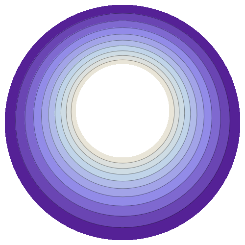
(b) Ring domain: Solution of the Dirichlet problem with contour lines.

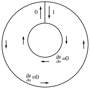
(c) Conjugate problem for the cut domain with new Dirichlet data along the both sides of the cut.

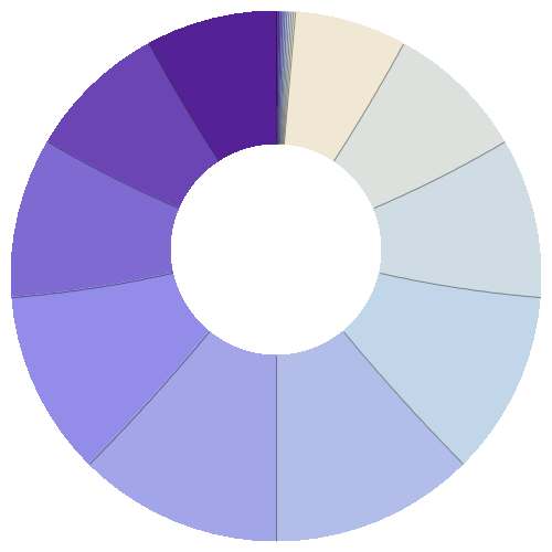
(d) Conjugate problem: Solution of the conjugate problem with contour lines.

(e) Mapped annulus.

Figure 2. Conjugate Function Method for Ring Domains.

4. Implementation Aspects

The $hp$-FEM implementation we are using is described in detail in [11]. For elliptic problems, the superior accuracy of the higher order methods with relatively small number of unknowns has to be balanced against the much higher integration cost and the cost of evaluating the solution at any given point in the domain. It should be emphasized though, that the conjugate function method is not dependent on any particular numerical PDE solution technique. Indeed, we fully expect that similar results could be obtained with, for instance, fine-tuned integral equation solvers.

In the context of solution of the conjugate pair problems, it is obvious that we have to integrate only once. Moreover, the factorization of the resulting discretized systems can be, for the most part, used in both problems without any extra work. Therefore, although in principle two problems are solved, in practice the work is almost proportional to that of one.

However, the computation of the contour lines necessarily involves a large number of evaluations of the solution, that also become more expensive as the order of the method increases.

4.1. $\boldsymbol{hp}$ -FEM

Here we give a short overview of the $hp$-FEM following closely to the one in [11]. In the $p$-version of the FEM the polynomial degree $p$ is used to control the accuracy of the solution while keeping the mesh fixed in contrast to the $h$-version or standard finite element method, where the polynomial degree is constant but the mesh size varies. Thus, the $p$-version is often referred to as the $p$-extension. The $hp$-method simply combines the $h$- and $p$- refinements.

These different refinement strategies also imply different sets of unknowns or degrees of freedom: In the $h$-version or the standard finite element method, the unknowns or degrees of freedom are associated with values at specified locations of the discretization of the computational domain, that is, the nodes of the mesh. In the $p$-method, the unknowns are coefficients of some polynomials that are associated with topological entities of the elements, nodes, sides, and the interior.

For optimal $hp$-convergence one should refine the mesh geometrically toward corners and let the degree of polynomial shape functions increase with distance from the corners. For an example of such a mesh see Figure 4. In the examples computed below, we have used a constant value of the order over the whole mesh.

In the following one way to construct a $p$-type quadrilateral element is given. The construction of triangles follows similar lines. First of all, the choice of shape functions is not unique. We use the so-called hierarchic integrated Legendre shape functions.

Legendre polynomials of degree $n$ can be defined by a recursion formula

$$(n+1)P_{n+1}(x)-(2n+1)xP_{n}(x)+nP_{n-1}(x)=0,$$

where $P_{0}(x)=1$ and $P_{1}(x)=x$.

The derivatives can similarly be computed by using the recursion

$$(1-x^{2})P^{\prime}_{n}(x)=-nxP_{n}(x)+nP_{n-1}(x).$$

The integrated Legendre polynomials are defined for $x\in[-1,1]$ as

$$\phi_{n}(\xi)=\sqrt{\frac{2n-1}{2}}\int_{-1}^{\xi}P_{n-1}(t)\,dt,\quad n=2,3,\ldots,$$

and can be rewritten as linear combinations of Legendre polynomials

$$\phi_{n}(\xi)=\frac{1}{\sqrt{2(2n-1)}}\left(P_{n}(\xi)-P_{n-2}(\xi)\right),\quad n=2,3,\ldots.$$

The normalizing coefficients are chosen so that

$$\int_{-1}^{1}\frac{d\phi_{i}(\xi)}{d\xi}\frac{d\phi_{j}(\xi)}{d\xi}\,d\xi=\delta_{ij},\quad i,j\geq 2.$$

Using these polynomials we can now define the shape functions for a quadrilateral reference element over the domain $[-1,1]\times[-1,1]$. The shape functions are divided into three categories: nodal shape functions, side modes, and internal modes.

There are four nodal shape functions.

$$N_{1}(\xi,\eta) =\frac{1}{4}(1-\xi)(1-\eta),\quad N_{2}(\xi,\eta)=\frac{1}{4}(1+\xi)(1-\eta),$$

$$N_{3}(\xi,\eta) =\frac{1}{4}(1+\xi)(1+\eta),\quad N_{4}(\xi,\eta)=\frac{1}{4}(1-\xi)(1+\eta),$$

which taken alone define the standard four-node quadrilateral finite element. There are $4(p-1)$ side modes associated with the sides of a quadrilateral $(p\geq 2)$, with $i=2,\ldots,p$,

$$N_{i}^{(1)}(\xi,\eta) =\frac{1}{2}(1-\eta)\phi_{i}(\xi),\quad N_{i}^{(2)}(\xi,\eta)=\frac{1}{2}(1+\xi)\phi_{i}(\eta),$$

$$N_{i}^{(3)}(\xi,\eta) =\frac{1}{2}(1+\eta)\phi_{i}(\eta),\quad N_{i}^{(4)}(\xi,\eta)=\frac{1}{2}(1-\xi)\phi_{i}(\xi).$$

For the internal modes we choose the $(p-1)(p-1)$ shape functions

$$N_{i,j}^{0}(\xi,\eta)=\phi_{i}(\xi)\phi_{j}(\eta),\quad i=2,\ldots,p,\quad j=2,\ldots,p.$$

The internal shape functions are often referred to as bubble-functions.

Note that some additional book-keeping is necessary. The Legendre polynomials have the property $P_{n}(-x)=(-1)^{n}P_{n}(x)$. This means that every edge must be globally parameterized in the same way in both elements to where it belongs. Otherwise unexpected cancellation in the degrees of freedom associated with the odd edge modes could occur.

4.2. Solution of Linear Systems

Let us divide the degrees of freedom of a discretized quadrilateral into five sets, internal and boundary degrees of freedom. The sets are denoted $B,D_{0},D_{1},N^{0}$, and $N^{1}$, for internal, Dirichlet $u=0$, Dirichlet $u=1$, Neumann with Dirichlet $u=0$ in the conjugate problem, and Neumann with Dirichlet $u=1$ in the conjugate problem, degrees of freedom, respectively.

The discretized system is

$$A=\begin{pmatrix}A_{BB}&A_{BN^{1}}&A_{BN^{0}}&A_{BD_{1}}&A_{BD_{0}}\\ A_{N^{1}B}&A_{N^{1}N^{1}}&A_{N^{1}N^{0}}&A_{N^{1}D_{1}}&A_{N^{1}D_{0}}\\ A_{N^{0}B}&A_{N^{0}N^{1}}&A_{N^{0}N^{0}}&A_{N^{0}D_{1}}&A_{N^{0}D_{0}}\\ A_{D_{1}B}&A_{D_{1}N^{1}}&A_{D_{1}N^{0}}&A_{D_{1}D_{1}}&A_{D_{1}D_{0}}\\ A_{D_{0}B}&A_{D_{0}N^{1}}&A_{D_{0}N^{0}}&A_{D_{0}D_{1}}&A_{D_{0}D_{0}}\\ \end{pmatrix}.$$

Taking the Dirichlet boundary conditions into account, we arrive at the following system of equations, using $x_{D_{1}}=\mathbf{1}$,

$$\begin{pmatrix}A_{BB}&A_{BN^{1}}&A_{BN^{0}}\\ A_{N^{1}B}&A_{N^{1}N^{1}}&A_{N^{1}N^{0}}\\ A_{N^{0}B}&A_{N^{0}N^{1}}&A_{N^{0}N^{0}}\\ \end{pmatrix}\begin{pmatrix}x_{B}\\ x_{N^{1}}\\ x_{N^{0}}\\ \end{pmatrix}=-\begin{pmatrix}A_{BD_{1}}\mathbf{1}\\ A_{N^{1}D_{1}}\mathbf{1}\\ A_{N^{0}D_{1}}\mathbf{1}\\ \end{pmatrix}.$$

For the conjugate problem, simply change the roles of $D_{1}\leftrightarrow N^{1}$ and $D_{0}\leftrightarrow N^{0}$. Note that $A_{BB}$ is present in both systems and thus has to be factored only once.

4.3. Evaluation of Contour Lines

Let $u$ and $v$ be solutions of the Dirichlet-Neumann problem and its conjugate problem, respectively. In computing the contour lines, the solutions and their gradients have to be evaluated at many points $(x,y)$. Evaluation of the solution in $hp$-FEM is more complicated than in the standard FEM. In a reference-element-based system such as ours, in order to evaluate the solution at point $(x,y)$ one must first find the enclosing element and then the local coordinates of the point on that element. Then every shape function has to be evaluated at the local coordinates of the point. This is outlined in detail in Algorithm 4.1. Similarly evaluation of the gradient of the solution requires two polynomial evaluations per one geometric search.

Algorithm 4.1.

(Evaluation of $u(x,y)$)

1. Find the enclosing element of $(x,y)$.

2. Find the local coordinates $(\xi,\eta)$ on the element.

3. Evaluate the shape functions $\phi_{i}(\xi,\eta)$.

4. Compute the linear combination of the shape functions $\sum_{i}c_{i}\phi_{i}(\xi,\eta)$, where $c_{i}$ are the coefficients from the solution vector.

Finding the images of the canonical domains is equivalent to finding the corresponding contour lines of $u$ and $v$. Since both solutions have been computed on the same mesh, evaluating the solutions and their gradients at the same point is straightforward. In Algorithm 4.2 the two-level line search is described in detail.

Algorithm 4.2.

(Tracing of Contour Lines: $u(x,y)=c=\text{const}$.)

1. Find the solutions $u(x,y)$ and $v(x,y)$.

2. Set the step size $\sigma$ and the tolerance $\epsilon$.

3. Choose the potential $c$.

4. Search along the Neumann boundary for the point $(x,y)$ such that $u(x,y)~{}=~{}c$.

5. Take a step of length $\sigma$ along the contour line of $u(x,y)$ in the direction of $\nabla v(x,y)$ to a new point $(\hat{x},\hat{y})$.

6. Correct the point $(\hat{x},\hat{y})$ by searching in the orthogonal direction, i.e., $\nabla u(\hat{x},\hat{y})$, until $|u(\hat{x},\hat{y})-c|<\epsilon$ is achieved.

7. Set $(x,y)=(\hat{x},\hat{y})$ and repeat until the opposite Neumann boundary has been reached.

4.4. On Computational Complexity

The solution time of a single problem can be divided into three parts, the setting up of the problem, the solution of the Dirichlet-Neumann and its conjugate problem, and the evaluation of the mappings. In short, in the absence of fully automatic mesh generators for this class of problems, the setting up of the problem remains the most time consuming part. We have implemented the algorithm using Mathematica 8.

The time and memory requirements, in terms of degrees of freedom, have been reported for the Dirichlet-Neumann problems in [11]. In the examples below, the solution times vary from few seconds to at most two minutes on standard hardware (as defined in Table 1). It should be noted that for comparable accuracy on polygonal domains, the Schwarz-Christoffel toolbox is superior to our implementation.

Table 1. Effect of $p$ and $\epsilon$ on contour lines computations. In geometry of Figure 10, ten contours of (radial) $u(x,y)=c_{u}$ and (circular) $v(x,y)=c_{v}$ have been computed with $\sigma=1/4$. Times are normalized so that for $p$=8, $\epsilon$ = 1/100, time $=1$. The time units are thus 1s and 46s for radial and circular contours, respectively. (Apple Mac Pro 2009 Edition 2.26 GHz, Mathematica 8.0.4)

$p$	$\epsilon$	time for $u(x,y)=c_{u}$	time for $v(x,y)=c_{v}$
4	1/100	0.44	0.43
4	1/1000	0.41	0.77
4	1/10000	1.51	1.19
8	1/100	1	1
8	1/1000	1.00	1.82
8	1/10000	0.99	2.66
12	1/100	2.29	2.31
12	1/1000	2.26	4.16
12	1/10000	2.26	6.07

Estimating the computational complexity of the mappings is complicated, since in the end, the chosen resolution of the image is the dominant factor for the time required. In Table 1, the effects of the polynomial degree and the chosen tolerance on the overall execution time are described. As a test case, a grid similar to one in Figure 10, has been computed by using $\sigma=0.25$ and $\epsilon=1/100,1/1000,1/10000$, for $p=4,8,12$. Note that for the radial contours the effect of $\epsilon$ is not as noticeable as for the circular ones due to contours and gradients being aligned.

5. Numerical Experiments

Our numerical experiments are divided into three different categories. First we validate the algorithm against the results obtained by the Schwarz-Christoffel toolbox and the analytic formula. Then we study several examples of using our method to construct conformal mappings from simply (see Figures 6–9) or doubly connected (see Figures 11–15) domains onto canonical domains, see Figure 3, with the main results summarized in Tables 2 and 3, respectively.

Table 2. Summary of the tests on simply connected domains. Accuracy is given as $\lceil\log_{10}|1-\textrm{M}(Q)\textrm{M}(\tilde{Q})|\rceil.$ For the first two cases the moduli are known due to symmetry.

Example	ID	$\textrm{M}(Q)$ / $\textrm{M}(\tilde{Q})$	Accuracy	Figure
Unit Disk	5.1	1 / 1	-13	6
Flower	5.2	1 / 1	-10	7
Circular quadrilateral	5.3	$0.63058735108478$ /	-13	8
		$1.585823119159254$
Asteroid cusp	5.4	$0.68435408764536$ /	-9	9
		$1.4612318657235575$

Table 3. Summary of the tests on ring domains. Accuracy is given as $\lceil\log_{10}|1-\textrm{M}(Q)\textrm{M}(\tilde{Q})|\rceil$, where the quadrilaterals are the cut domains.

Example	ID	$\textrm{M}(R)$	Accuracy	Figure
Disk in regular pentagon	5.5	See Table 5.		10
Cross in square	5.6	$0.2862861647287473$	-9	11
Circle in square	5.7	$0.9920378629010557$	-13	12
Flower in square	5.8	$0.6669554623348065$	-8	13
Circle in L	5.9	$1.0935085836560234$	-9	14
Droplet in square	5.10	$0.8979775098918368$	-9	15

Figure 3. Canonical domains $R_{h}$ and $A_{r}$ on the left- and right-hand side, respectively.

5.1. Setup of the Validation Test

Validation of the algorithm for the conformal mapping will be carried out in two cases, first we compare our algorithm with SC Toolbox in a convex and a non-convex quadrilateral. In the second test we parameterized the modulus of a rectangle and map it onto the unit disk.

The comparison to the SC Toolbox is carried out in the following quadrilaterals: convex quadrilateral $(\Omega;0,1,1.5+1.5i,i)$ and non-convex quadrilateral $(\Omega;0,1,0.3+0.3i,i)$, and line-segments joining the vertices as the boundary arcs. Then comparisons of the results obtained by the conjugate function method, presented in this paper, and SC Toolbox by Driscoll [8] are carried out. All SC Toolbox tests were carried with the settings precision = 1e-14. Comparison is done by using the following test function

$$\textrm{test}(z)=|f(z)-g(z)|,$$ (3)

where $f$ and $g$ are obtained by the conjugate function method and SC Toolbox, respectively. The mesh setup of the quadrilaterals and the results of the test function (3) are shown in Figure 4 and 5, respectively.

Figure 4. Geometric mesh of the convex (left-hand side) and the non-convex (right-hand side) quadrilateral used in computing the potential functions.

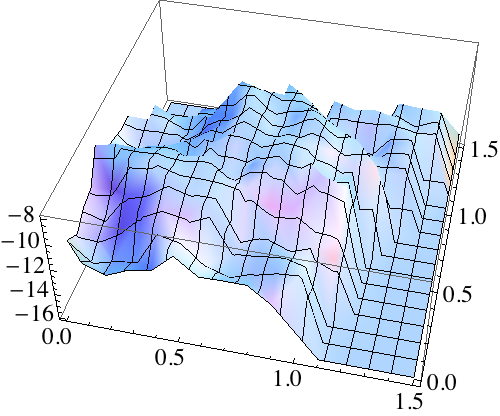
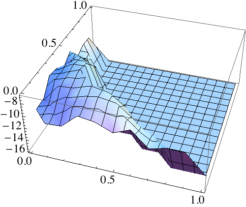
Figure 5. Comparison of the convex (left-hand side) and non-convex (right-hand side) quadrilateral between the conjugate function method and SC Toolbox. Results are obtained by taking the logarithm (with base 10) of the test function (3).

All our examples are carried out in the same fashion using the reciprocal identity (1) and a quadrilateral $Q$. The test function is

$$\textrm{rec}(Q)=|\textrm{M}(Q)\,\textrm{M}(\tilde{Q})-1|,$$

which vanishes identically. See also [11, Section 4].

In the second validation test, we parameterized a rectangle with respect to the modulus $\textrm{M}(Q)$ and map the rectangle onto the unit disk. The mapping is given by a composite mapping consisting of a Jacobi’s elliptic sine function and a Möbius transformation.

For every point $(x_{j},y_{j})$ in the grid on the rectangle $R_{h}$, where $x_{j}=j/10$ and $y_{j}=jh/10$, $j=0,1,2,\ldots,10$, we compute the error $\|e_{j}\|$ which is simply the Euclidean distance of the image of the initial point $(x_{j},y_{j})$ computed by the conjugate function method and the analytical mapping. For a given modulus $\textrm{M}(Q)$ the values $\textrm{rec}(Q)$, $\max(\|e_{j}\|)$, and $\textrm{mean}(\|e_{j}\|)$, where the latter two represent the maximal and the mean error over the grid are presented in Table 4.

Note that our test function $\textrm{rec}(Q)$ effectively measures the error in energy. Given the very high accuracy of the results obtained, we are confident that even though no a priori guarantees for pointwise convergence can be given, the second test is a valid indication of the global convergence behavior.

Table 4. The values of $\textrm{rec}(Q)$, $\max(\|e_{j}\|)$ and $\textrm{mean}(\|e_{j}\|)$ for a given $\textrm{M}(Q)$.

$\textrm{M}(Q)$	$\textrm{rec}(Q)$	$\max(\|e_{j}\|)$	$\textrm{mean}(\|e_{j}\|)$
$1$	$8.08242\cdot 10^{-14}$	$1.87409\cdot 10^{-8}$	$5.56947\cdot 10^{-10}$
$1.2$	$6.35048\cdot 10^{-14}$	$7.97889\cdot 10^{-9}$	$7.49315\cdot 10^{-10}$
$1.4$	$5.52891\cdot 10^{-14}$	$1.21851\cdot 10^{-8}$	$6.90329\cdot 10^{-10}$
$1.6$	$8.85958\cdot 10^{-14}$	$1.10001\cdot 10^{-8}$	$7.90840\cdot 10^{-10}$
$1.8$	$9.72555\cdot 10^{-14}$	$1.19005\cdot 10^{-8}$	$7.31645\cdot 10^{-10}$
$2$	$9.41469\cdot 10^{-14}$	$8.56068\cdot 10^{-9}$	$7.67815\cdot 10^{-10}$

5.2. Simply Connected Domains

In this section we consider a conformal mapping of a quadrilateral $Q=(\Omega;z_{1},z_{2},z_{3},z_{4})$ with curved boundaries $\gamma_{1},\gamma_{2},\gamma_{3}$, $\gamma_{4}$ onto a rectangle $R_{h}$ such that the vertices $z_{1},z_{2},z_{3},z_{4}$ maps to $1+ih,ih,0,1$, respectively, and the boundary curves $\gamma_{1},\gamma_{2},\gamma_{3},\gamma_{4}$ maps onto the line segments $\gamma_{1}^{\prime},\gamma_{2}^{\prime},\gamma_{3}^{\prime},\gamma_{4}^{\prime}$. We give some examples and applications with illustrations. Simple examples of such domains are domains, where four or more points are connected with circular arcs. Some examples related to numerical methods and the Schwarz-Christoffel formula for such domains can be found in the literature, e.g., [6, 7, 16].

Example 5.1 (Unit disk).

Let $\Omega$ be the unit disk. We consider a quadrilateral $Q=(\Omega;z_{1},z_{2},z_{3},z_{4})$, where $z_{j}=e^{i\theta_{j}}$, $\theta_{j}=(j-1)\pi/2$. Note that, because of the symmetry, it follows from (1) that the modulus is $1$. The reciprocal error of the conformal mappings is $4.34\cdot 10^{-14}$. This example was first given by Schwarz in 1869 [24].

Figure 6. Example of the conformal map of a square onto a disk, first obtained by Schwarz in 1869 [24].

Example 5.2 (Flower).

Let $\Omega$ be the domain bounded by the curve

$$r(\theta)=0.8+t\cos(n\theta),$$ (4)

where $0\leq\theta\leq 2\pi$, $n=6$ and $t=0.1$. We consider a quadrilateral $Q=(\Omega;z_{1},z_{2},z_{3},z_{4})$, where $z_{j}=r(\theta_{j})$, $\theta_{j}=(j-1)\pi/2$; see Figure 7. As in Example 5.1, the modulus of $Q$ is 1. The reciprocal error of the conformal mappings is $3.74\cdot 10^{-11}$. Several other examples of flower shaped quadrilaterals are given in [11, Section 8.5].

Figure 7. Illustration of the flower domain and the visualization of the pre-image of the rectangular grid (Figure 3).

Example 5.3 (Circular Quadrilateral).

In [11] several experiments of circular quadrilaterals are given. Let us consider a quadrilateral whose sides are circular arcs of intersecting orthogonal circles, i.e., angles are $\pi/2$. Let $0<a<b<c<2\pi$ and choose the points $\{1,e^{ia},e^{ib},e^{ic}\}$ on the unit circle. Let $Q_{A}$ stand for the domain which is obtained from the unit disk by cutting away regions bounded by the two orthogonal arcs with endpoints $\{1,e^{ia}\}$ and $\{e^{ib},e^{ic}\}$, respectively. Then $Q_{A}$ determines a quadrilateral $(Q_{A};e^{ia},e^{ib},e^{ic},1)$. Then for the triple $(a,b,c)=(\pi/12,17\pi/12,3\pi/2)$, the modulus $\textrm{M}(Q_{A})=0.630587351084775$ and $\textrm{M}(\tilde{Q}_{A})=1.5858231191592544$. The reciprocal error of the conformal mapping is $1.68\cdot 10^{-13}$.

Figure 8. The quadrilateral $(Q_{A};e^{i\pi/12},e^{i17\pi/12},e^{i3\pi/2},1)$ and the visualization of the pre-image of the rectangular grid (Figure 3).

Example 5.4 (Asteroid Cusp).

Asteroid cusp is a domain $\Omega$ given by a

$$G_{c}=\{(x,y):|x|<c,\,|y|<c\},$$ (5)

where $c=1$ and the left-hand side vertical boundary line-segment is replaced by the following curve

$$r(t)=-1+\cos^{3}t+i\sin^{3}t,\ t\in[-\pi/2,\pi/2].$$

We consider a quadrilateral $Q=(\Omega;1-i,\,1+i,\,-1+i,\,-1-i)$. The reciprocal error of the conformal mappings is of the order $10^{-10}$. The modulus $\textrm{M}(Q)=0.68435408764536$ and $\textrm{M}(\tilde{Q})=1.4612318657235575$. The domain is illustrated in Figure 9.

Figure 9. Asteroid cusp domain with the pre-image of the rectangular grid (Figure 3).

5.3. Ring Domains

In this section we shall give several examples of conformal mapping from a ring domain $R$ onto an annulus $A_{r}$. It is also possible to use the Schwarz-Christoffel method, see [13]. For symmetrical ring domains a conformal mapping can be obtained by using Schwarz’ symmetries.

Example 5.5 (Disk in Regular Pentagon).

Let $\Omega$ be a regular pentagon centered at the origin and having short radius (apothem) equal to $1$ such that the corners of the pentagon are $z_{k}=\sec(\pi/5)e^{2\pi ik/5}$, $k=0,1,2,3,4$. Let $\mathbb{D}(r)=\{z\in\mathbb{C}:|z|\leq r\}$. We consider a ring domain $R=\Omega\backslash\mathbb{D}(r)$ and compute the modulus $\textrm{M}(R)$ and the exponential of the modulus $e^{\textrm{M}(R)}$. Results are reported in Table 5 with the values $e^{\textrm{M}(R)}$ from [3, Example 5] in the fourth column.

Table 5. The values $\textrm{M}(R)$ and $e^{\textrm{M}(R)}$.

$r$	$\textrm{M}(R)$	$\exp(\textrm{M}(R))$	[3, Example 5]
$0.1$	$2.35372035858745$	$10.524652459913115$	$10.5246525$
$0.4$	$0.9674246001764809$	$2.631159438480101$	$2.631159439$
$0.9$	$0.15070188000332954$	$1.1626499971978235$	$1.1626499972$
$0.99$	$0.03276861064365647$	$1.0333114143138304$	$1.03331141431$
$0.999$	$0.00934656029871744$	$1.0093903757950962$	$1.00939037579$

Figure 10. Disk in pentagon $(r=0.4)$ with the pre-image of the annular grid (Figure 3).

Example 5.6 (Cross in Square).

Let $G_{ab}=\{(x,y):|x|\leq a,\,|y|\leq b\}\cup\{(x,y):|x|\leq b,\,|y|\leq a\}$, and $G_{c}$ as in (5), where $a<c$ and $b<c$. Then the domain cross in square is a ring domain $R=G_{c}\backslash G_{ab}$, see Figure 11. The reciprocal error of the conformal mapping is of the order $10^{-10}$. The modulus $\textrm{M}(R)=0.2862861647287473$.

Figure 11. The ring domain $G_{c}\backslash G_{ab}$, where $a=0.5,b=1.2,c=1.5$, with the pre-image of the annular grid (Figure 3).

Example 5.7 (Circle in Square).

Let $\Omega$ be the unit disk. Then we consider a ring domain $R=G_{c}\backslash\Omega$, where $c=1.5$, see Figure 12. The reciprocal error of the conformal mapping is of the order $10^{-14}$. The modulus $\textrm{M}(R)=0.9920378629010557$.

Figure 12. Disk in a square domain with the pre-image of the annular grid (Figure 3).

Example 5.8 (Flower in Square).

Let $\Omega$ be a domain bounded by the curve (4). Then we consider a ring domain $R=G_{c}\backslash\Omega$, where $G_{c}$ is given by (5) and $c=1.5$. See Figure 13 for the illustration. The reciprocal error of the conformal mapping is of the order $10^{-9}$. The modulus $\textrm{M}(R)=0.6669554623348065$.

Figure 13. Flower in a square domain with the pre-image of the annular grid (Figure 3).

Example 5.9 (Circle in L).

Let $L_{1}=\{z\in\mathbb{C}:0<\textrm{Re}(z)<a,\,0<\textrm{Im}(z)<b\}$ and $L_{2}=\{z\in{\mathbb{C}}:0<\textrm{Re}(z)<d,\,0<\textrm{Im}(z)<c\}$, where $0<d<a,\;0<b<c$. Then $L(a,b,c,d)=L_{1}\cup L_{2}$ is called an L-domain. Suppose that $\mathbb{D}(z_{0},r)=\{z\in\mathbb{C}:|z-z_{0}|<r\}$. We consider a ring domain $R=L(a,b,c,d)\backslash\mathbb{D}(z_{0},r)$, where $(a,b,c,d)=(3,1,2,1)$, $z_{0}=8/5+2i/5$, and $r=1/5$. See Figure 14.

In order to better illustrate the details of the mapping, a non-uniform grid has been used. For the real component the points $x$ are

$$x=\{k/10\ :\ k=0,1,\ldots,9\}\cup\{99/100,999/10000,9999/10000,1\}.$$

For the imaginary component the points $y$ are chosen on purely aesthetic basis as:

$$y=\{k/10\ :\ k=1,2,\ldots,9\} \ \cup$$

$$\{0.316225,0.324008, 0.327831,0.329278,0.331005,0.687482\}.$$

The reciprocal error of the conformal mapping is of the order $10^{-10}$. The modulus $\textrm{M}(R)=1.0935085836560234$.

Figure 14. L-shaped domain with a circular hole with the pre-image of the non-uniform annular grid of Example 5.9.

Example 5.10 (Droplet in Square).

Let $Q_{D}$ be bounded by a Bezier curve:

$$r(t)=\frac{1}{640}\left(45t^{6}+75t^{4}-525t^{2}+469\right)+\frac{15}{32}t\left(t^{2}-1\right)^{2}i,\ t\in[-1,1].$$

Then the domain droplet in square is a ring domain $R=G_{c}\backslash Q_{D}$, where $G_{c}$ in given in the first example concerning ring domains. For visualization, see Figure 15. The reciprocal error of the conformal mapping is of the order $10^{-10}$. The modulus $\textrm{M}(R)=0.8979775098918368$.

Figure 15. Droplet in square with the pre-image of the annular grid (Figure 3).

Acknowledgment.

We thank T.A. Driscoll, R.M. Porter and M. Vuorinen for their valuable comments on this paper.

References

- [1] L.V. Ahlfors, Conformal invariants: topics in geometric function theory, McGraw-Hill Book Co., 1973.
- [2] L.V. Ahlfors, Complex Analysis, An introduction to the theory of analytic functions of one complex variable, Third edition. International Series in Pure and Applied Mathematics. McGraw-Hill Book Co., New York, 1978.
- [3] D. Betsakos, K. Samuelsson and M. Vuorinen, The computation of capacity of planar condensers, Publ. Inst. Math., Vol. 75 (89) (2004), 233–252.
- [4] P.L. Bowers and M.K. Hurdal, Planar Conformal Mappings of Piecewise Flat Surfaces, In Visualization and Mathematics III, 3–34, 2003.
- [5] J. Brandts, The Cauchy-Riemann equations: discretization by finite elements, fast solution of the second variable, and a posteriori error estimation, A posteriori error estimation and adaptive computational methods. Adv. Comput. Math., Vol. 15 (2001), No. 1-4, 6177 (2002).
- [6] P.R. Brown, Mapping onto circular arc polygons, Complex Variables, Theory Appl., Vol. 50 (2005), No. 2, 131–154.
- [7] P.R. Brown and R.M. Porter, Conformal Mapping of Circular Quadrilaterals and Weierstrass Elliptic Functions, Comput. Methods Funct. Theory, Vol. 11 (2011), No. 2, 463–486.
-
[8]
T.A. Driscoll,
Schwarz-Christoffel toolbox for MATLAB,
http://www.math.udel.edu/~driscoll/SC/ - [9] T.A. Driscoll and L.N. Trefethen, Schwarz-Christoffel Mapping, Cambridge Monographs on Applied and Computational Mathematics, 8. Cambridge University Press, 2002.
- [10] T.A. Driscoll and S.A. Vavasis, Numerical conformal mapping using cross-ratios and Delaunay triangulation, SIAM J. Sci. Comput., Vol. 19 (1998), No. 6, 1783–1803.
- [11] H. Hakula, A. Rasila, and M. Vuorinen, On moduli of rings and quadrilaterals: algorithms and experiments, SIAM J. Sci. Comput., Vol. 33 (2011), No. 1, 279–302.
- [12] P. Henrici, Applied and computational complex analysis. Vol. 3, Discrete Fourier analysis—Cauchy integrals—construction of conformal maps—univalent functions. Pure and Applied Mathematics (New York). A Wiley-Interscience Publication. John Wiley & Sons, Inc., New York, 1986.
- [13] C. Hu, Algorithm 785: a software package for computing Schwarz-Christoffel conformal transformation for doubly connected polygonal regions, ACM Transactions on Mathematical Software (TOMS), Vol. 24 (1998), No. 3, 317–333.
- [14] L. Kharevych, B. Springborn, and P. Schröder, Discrete conformal mappings via circle patterns, ACM Transactions on Graphics (TOG), Vol. 25 (2006), No. 2, 412–423.
- [15] S.V. Krantz, Geometric Function Theory, Explorations in complex analysis. Cornerstones. Birkhuser Boston, Inc., Boston, MA, 2006.
- [16] V.V. Kravchenko and R.M. Porter, Conformal mapping of right circular quadrilaterals, Complex Variables and Elliptic Equations: An International Journal, iFirst (2010), 1–17.
- [17] P.K. Kythe, Computational conformal mapping, Birkhuser Boston, Inc., Boston, MA, 1998.
- [18] O. Lehto and K.I. Virtanen, Quasiconformal mappings in the plane, Springer, Berlin, 1973.
- [19] D.E. Marshall, Zipper, Fortran Programs for Numerical Computation of Conformal Maps, and C Programs for X-11 Graphics Display of the Maps. Sample pictures, Fortran, and C code available online at http://www.math.washington.edu/~marshall/personal.html.
- [20] D.E. Marshall and S. Rohde, Convergence of a variant of the zipper algorithm for conformal mapping, SIAM J. Numer. Anal., Vol. 45 (2007), No. 6, 2577–2609 (electronic).
- [21] N. Papamichael and N.S. Stylianopoulos, Numerical Conformal Mapping: Domain Decomposition and the Mapping of Quadrilaterals, World Scientific Publishing Company, 2010.
- [22] R.M. Porter, History and Recent Developments in Techniques for Numerical Conformal Mapping, Quasiconformal Mappings and their Applications (ed. by S. Ponnusamy, T. Sugawa and M. Vuorinen), Narosa Publishing House Pvt. Ltd., New Delhi, India (2007), 207–238.
- [23] R. Schinzinger and P.A.A. Laura, Conformal mapping: methods and applications, Revised edition of the 1991 original. Dover Publications, Inc., Mineola, NY, 2003.
- [24] H.A. Schwarz, Conforme Abbildung der Oberfläche eines Tetraeders auf die Oberfläche einer Kugel, J. Reine Ange. Math., Vol. 70 (1869), 121–136.
- [25] L.N. Trefethen, Numerical computation of the Schwarz-Christoffel transformation, SIAM J. Sci. Statist. Comput., Vol. 1 (1980), No. 1, 82–102.