Nonequilibrium Keldysh Formalism for Interacting Leads – Application to Quantum Dot Transport Driven by Spin Bias

Abstract

The conductance through a mesoscopic system of interacting electrons coupled to two adjacent leads is conventionally derived via the Keldysh nonequilibrium Green’s function technique, in the limit of noninteracting leads [see Y. Meir et al., Phys. Rev. Lett. 68, 2512 (1991)]. We extend the standard formalism to cater for a quantum dot system with Coulombic interactions between the quantum dot and the leads. The general current expression is obtained by considering the equation of motion of the time-ordered Green’s function of the system. The nonequilibrium effects of the interacting leads are then incorporated by determining the contour-ordered Green’s function over the Keldysh loop and applying Langreth’s theorem. The dot-lead interactions significantly increase the height of the Kondo peaks in density of states of the quantum dot. This translates into two Kondo peaks in the spin differential conductance when the magnitude of the spin bias equals that of the Zeeman splitting. There also exists a plateau in the charge differential conductance due to the combined effect of spin bias and the Zeeman splitting. The low-bias conductance plateau with sharp edges is also a characteristic of the Kondo effect. The conductance plateau disappears for the case of asymmetric dot-lead interaction.

1 Introduction

With the advancement in nanotechnology, a small number of interacting electrons can be confined in a quantum dot, to mimic the behavior of impurity atoms in a metal, thus enabling the study of many-body correlations between electrons. One such many-body phenomenon is the Kondo effect, the discovery of which in quantum dot systems [1, 2], has generated tremendous theoretical [3, 4, 5, 6] and experimental [7, 8] interest. Early works on the Kondo effect had largely focused on the effect of charge bias which applied to the two leads. Later, attentions have shifted to the Kondo effects of the systems including ferromagnetic leads [9, 10, 11, 12] and the leads with spin accumulation [13]. Spin accumulation is the nonequilibrium split in the chemical potentials of spin-up and spin-down electrons. Accordingly, a spin bias can be realized experimentally, for instance, by controlling the spin accumulation at the biased contacts between ferromagnetic and nonmagnetic leads, and can in turn, generate a pure spin current without any accompanying charge current [14, 15]. Recent experimental progress has opened new possibilities for the study of spin-bias-induced transport in strongly correlated systems [16, 17, 18]. However the effect of the spin bias on the Kondo effect remains largely unexplored. More importantly, the Kondo effect in the presence of Coulombic interactions between the quantum dot and two adjacent leads has not been studied.

Such dot-lead interactions warrant an investigation owing to the increasing influence of leads with the reduction in the lead-dot separation. The nonequilibrium (bias-driven) transport through a interacting mesoscopic system is usually modeled by the Keldysh nonequilibrium Green’s function (NEGF) method. The standard Keldysh NEGF method for a central quantum dot system coupled to two biased leads, was first developed by Meir et al. [19], and widely applied thereafter [20, 21, 22, 23, 24].

In this paper, we derive the general analytical expression for the current in a quantum dot system with interacting leads. The dot-lead Coulombic interactions are then incorporated by determining the contour-ordered Green’s function over the Keldysh loop and applying Langreth’s theorem. Based on the current formula, and the retarded Green’s function of the quantum dot system, we study the low-temperature spin transport and the Kondo physics induced by a spin bias, in the presence of dot-lead Coulombic interactions. Two sharp peaks occur in the density of states in the Kondo regime. This translates into Kondo peaks occur in the spin differential conductance when the magnitude of the spin bias becomes equal to that of the Zeeman split of the quantum dot energy levels. There also exists a conductance plateau in the charge differential conductance at low bias, due to the combined effect of the spin bias and the Zeeman splitting. Since the Kondo effect primarily arises from intra-dot Coulomb interactions between electrons of opposite spins, the Kondo peaks and hence the position of the conductance peaks and plateau are largely unaffected by the strength of the lead-dot Coulombic interactions. The conductance plateau disappears when the symmetry between the dot-lead interactions in the left and right junctions is broken.

The organization of the rest of the paper is as follows. In Sec. 2, the Hamiltonian of the system is introduced, and the current formula and corresponding Green’s functions are derived. In Sec. 3, we present the results of our numerical calculation of density of states and the differential conductance in the presence of the dot-lead Coulombic interactions. Finally, a brief summary is given in Sec. 4.

2 Model and formulation

The Hamiltonian of the quantum dot system can be written as $H=H_{c}+H_{cen}+H_{T}+H_{ld}$. The first term is the Hamiltonian of the contacts

$$H_{c}=\sum_{k\sigma\alpha\in\mathrm{L,R}}\varepsilon_{\alpha k\sigma}c_{\alpha k\sigma}^{{\dagger}}c_{\alpha k\sigma},$$ (1)

while the Hamiltonian of the central region is described by:

$$H_{cen}=\sum_{\sigma}\varepsilon_{\sigma}d_{\sigma}^{{\dagger}}d_{\sigma}+Ud_{\uparrow}^{{\dagger}}d_{\uparrow}d_{\downarrow}^{{\dagger}}d_{\downarrow},$$ (2)

where $c_{\alpha k\sigma}^{{\dagger}}$ ($c_{\alpha k\sigma}$) and $d_{\sigma}^{{\dagger}}$ ($d_{\sigma}$) are the creation (annihilation) operators of an electron with spin $\sigma(=\uparrow,\downarrow)$ in the lead $\alpha(=\mathrm{L,R})$ and the quantum dot, respectively. The second term in $H_{cen}$ is the Anderson term where $U$ refers to the on-site Coulombic repulsion, while $\varepsilon_{\alpha k\sigma}$ and $\varepsilon_{\sigma}$ are the energy levels of the two leads and the quantum dot, respectively. For simplicity, we consider only a single pair of levels with energies $\varepsilon_{\sigma}=\varepsilon_{0}+\sigma\Delta\varepsilon/2$. The third term represents tunneling coupling between the leads and the central region:

$$H_{T}=\sum_{k\sigma\alpha\in\mathrm{L,R}}(t_{\alpha\sigma}c^{{\dagger}}_{\alpha k\sigma}d_{\sigma}+\mathrm{H.C.}),$$ (3)

where $t_{\alpha\sigma}$ refers to the tunneling coupling constant.

In the conventional NEGF method, the interactions in the leads are disregarded so that the semi-infinite leads can be described by the simple noninteracting Green’s function (see Meir et al. [19]). In this paper, however, we incorporate the Coulombic interaction between the charges on the quantum dot and the two leads, which may be significant given the proximity of the two regions. This interaction term in the Hamiltonian $H_{ld}$ is given by[25]

$$H_{ld}=\sum_{\alpha k\sigma\sigma^{\prime}}I_{\alpha k}d_{\sigma}^{\dagger}d_{\sigma}c_{\alpha k\sigma^{\prime}}^{{\dagger}}c_{\alpha k\sigma^{\prime}},$$ (4)

where $I_{\alpha k}$ denotes the interaction strength. We first derive the general formula of the current by considering the equation of motion method, and the contour-ordered Green’s function over the Keldysh loop, as will be shown explicitly below.

The current from the lead $\alpha$ through barrier to the central region can be calculated from the time evolution of the occupation number operator of the lead $\alpha$:

$$J_{\alpha\sigma}=-e\langle\dot{N}_{\alpha\sigma}\rangle=\frac{2e}{\hbar}\mathrm{Re}\big{\{}\sum_{k}t_{\alpha\sigma}G_{\alpha k\sigma}^{<}(t,t)\big{\}},$$ (5)

where $N_{\alpha\sigma}=\sum_{k}c_{\alpha k\sigma}^{{\dagger}}c_{\alpha k\sigma}$ and the lesser Green’s function is defined as

$$G_{\alpha k\sigma}^{<}(t,t^{\prime})\equiv i\langle c_{\alpha k\sigma}^{{\dagger}}(t^{\prime})d_{\sigma}(t)\rangle.$$ (6)

According to the equation of motion satisfied by the time-ordered Green’s function $G_{\alpha k\sigma}^{t}$, namely,

$$-i\frac{\partial}{\partial t^{\prime}}G_{\alpha k\sigma}^{t}(t,t^{\prime})=\varepsilon_{\alpha k\sigma}G_{\alpha k\sigma}^{t}(t,t^{\prime})+t_{\alpha\sigma}^{\ast}G_{\sigma}^{t}(t,t^{\prime})$$

$$\hskip 14.22636pt+\sum_{\sigma^{\prime\prime}}I_{\alpha k}(-i)\langle\mathrm{T}\{d_{\sigma}(t)d_{\sigma^{\prime\prime}}^{\dagger}(t^{\prime})d_{\sigma^{\prime\prime}}(t^{\prime})c_{\alpha k\sigma}^{{\dagger}}(t^{\prime})\}\rangle,$$ (7)

where we define the central region time-ordered Green’s function $G_{\sigma}^{t}(t,t^{\prime})=-i\langle\mathrm{T}\{d_{\sigma}(t)d_{\sigma}^{\dagger}(t^{\prime})\}\rangle$ with $\mathrm{T}$ being the time-ordering operator. Note that the Coulombic interaction between the quantum dot and the leads results in the last term in Eq. (2). This additional term prevents the closure of the equation of motion satisfied by $G_{\alpha k\sigma}^{t}$ except by utilizing certain approximations. We adopt the Hartree-Fock approximation to deal with this term and obtain a closed set of equations. Using the Hartree-Fock approximation, the last term can be expressed as

$$-i\langle T\{d_{\sigma}(t)d_{\sigma^{\prime\prime}}^{\dagger}(t^{\prime})d_{\sigma^{\prime\prime}}(t^{\prime})c_{\alpha k\sigma}^{{\dagger}}(t^{\prime})\}\rangle\simeq n_{\sigma^{\prime\prime}}(-i)\langle T\{d_{\sigma}(t)c_{\alpha k\sigma}^{{\dagger}}(t^{\prime})\}\rangle,$$

here $n_{\sigma^{\prime\prime}}=\langle d_{\sigma^{\prime\prime}}^{\dagger}d_{\sigma^{\prime\prime}}\rangle$. Thus, the equation of motion of Eq. (2) can be rewritten as

$$\left[-i\frac{\partial}{\partial t^{\prime}}-\varepsilon_{\alpha k\sigma}-A_{\alpha k}\right]G_{\alpha k\sigma}^{t}(t,t^{\prime})=t_{\alpha\sigma}^{\ast}G_{\sigma}^{t}(t,t^{\prime}),$$ (8)

where $A_{\alpha k}=nI_{\alpha k}$ with $n=n_{\uparrow}+n_{\downarrow}$. Thus, the Green’s function $G_{\alpha k\sigma}^{<}(t,t^{\prime})$ can be derived through adopting Langreth’s theorem, namely

$$G_{\alpha k\sigma}^{<}(t,t^{\prime})=\int dt_{1}t_{\alpha\sigma}^{\ast}\big{[}G_{\sigma}^{r}(t,t_{1})g_{\alpha k\sigma}^{<}(t_{1},t^{\prime})+G_{\sigma}^{<}(t,t_{1})g_{\alpha k\sigma}^{a}(t_{1},t^{\prime})\big{]},$$ (9)

where the time-dependent Green’s function of the leads for the uncoupled system with the modified energy level $\varepsilon_{\alpha k\sigma}^{\prime}$ are

$$g_{\alpha k\sigma}^{<}(t,t^{\prime}) = if_{\alpha\sigma}(\varepsilon_{\alpha k\sigma}^{\prime})\exp\big{[}-i\varepsilon_{\alpha k\sigma}^{\prime}(t-t^{\prime})\big{]},$$ (10)

$$g_{\alpha k\sigma}^{(r,a)}(t,t^{\prime}) = \mp i\theta(\pm t\mp t^{\prime})\exp\big{[}-i\varepsilon_{\alpha k\sigma}^{\prime}(t-t^{\prime})\big{]},$$ (11)

where $f_{\alpha\sigma}(\varepsilon_{\alpha k\sigma}^{\prime})=\big{\{}\exp\big{[}(\varepsilon_{\alpha k\sigma}^{\prime}-\mu_{\alpha\sigma})/k_{B}T\big{]}+1\big{\}}^{-1}$. Substituting the Green’s function $G_{\alpha k\sigma}^{<}(t,t^{\prime})$ into Eq. (5), we can obtain the formula of the current

$$J_{\alpha\sigma} = \frac{ie}{\hbar}\int\frac{d\epsilon}{2\pi}\Gamma_{\alpha\sigma}(\epsilon)\big{\{}G_{\sigma}^{<}(\epsilon+A_{\alpha}(\epsilon))$$ (12)

$$+f_{\alpha\sigma}(\epsilon+A_{\alpha}(\epsilon))\big{[}G^{r}_{\sigma}(\epsilon+A_{\alpha}(\epsilon))-G^{a}_{\sigma}(\epsilon+A_{\alpha}(\epsilon))\big{]}\big{\}},$$

where $\Gamma_{\alpha\sigma}=2\pi\sum_{k}|t_{\alpha\sigma}|^{2}\delta(\epsilon-\varepsilon_{\alpha k\sigma})$ is the linewidth function and $A_{\alpha}(\epsilon)=nI_{\alpha}(\epsilon)$. The Green’s function $G^{r,<}_{\sigma}(\epsilon)$ are the Fourier transformations of $G^{r,<}_{\sigma}(t)$ with $G^{r}_{\sigma}(t)=-i\theta(t)\langle\{d_{\sigma}(t),d_{\sigma}^{\dagger}(0)\}\rangle\equiv\langle\langle d_{\sigma}(t)|d_{\sigma}^{\dagger}(0)\rangle\rangle^{r}$, $G^{<}_{\sigma}(t)=i\langle d^{\dagger}_{\sigma}(0)d_{\sigma}(t)\rangle\equiv\langle\langle d_{\sigma}(t)|d_{\sigma}^{\dagger}(0)\rangle\rangle^{<}$. For the case of proportionate coupling to the leads, i.e., $\Gamma_{L\sigma}=\lambda\Gamma_{R\sigma}$, the formula of the current can be simplified. Defining the current $J=xJ_{L}-(1-x)J_{R}$ with $J_{\alpha}=J_{\alpha\uparrow}+J_{\alpha\downarrow}$, we can obtain the simplified formula of the charge current, namely

$$J = \frac{e}{\hbar}\sum_{\sigma}\int d\epsilon\left[f_{L\sigma}(\epsilon+A_{\alpha}(\epsilon))-f_{R\sigma}(\epsilon+A_{\alpha}(\epsilon))\right]$$ (13)

$$\hskip 28.45274pt\times\frac{\Gamma_{L\sigma}(\epsilon)\Gamma_{R\sigma}(\epsilon)}{\Gamma_{L\sigma}(\epsilon)+\Gamma_{R\sigma}(\epsilon)}\left[-\frac{1}{\pi}\mathrm{Im}G^{r}_{\sigma}(\epsilon+A_{\alpha}(\epsilon))\right].$$

Thus, finally, the current can be expressed solely in terms of the retarded Green’s function.

We now proceed to solve the retarded Green’s function $G^{r}_{\sigma}(\epsilon)$. The standard equation of motion technique yields the following general relation

$$\epsilon\langle\langle\hat{F}_{1}|\hat{F}_{2}\rangle\rangle^{r}=\langle\{\hat{F}_{1},\hat{F}_{2}\}\rangle+\langle\langle\left[\hat{F}_{1},H\right]|\hat{F}_{2}\rangle\rangle^{r},$$

where $\hat{F}_{1}$ and $\hat{F}_{2}$ are arbitrary operators. Note that the energy $\epsilon$ includes a infinitesimal imaginary part $i0^{+}$. By considering the model Hamiltonian, the equation of motion of the Green’s function $G_{\sigma}^{r}(t)$ can thus be written as

$$(\epsilon-\varepsilon_{\sigma})\langle\langle d_{\sigma}|d_{\sigma}^{\dagger}\rangle\rangle^{r} = 1+\sum_{\alpha k\sigma^{\prime}}I_{\alpha k}\langle\langle d_{\sigma}c_{\alpha k\sigma^{\prime}}^{\dagger}c_{\alpha k\sigma^{\prime}}|d_{\sigma}^{\dagger}\rangle\rangle^{r}$$ (14)

$$+\sum_{\alpha k}t_{\alpha\sigma}^{\ast}\langle\langle c_{\alpha k\sigma}|d_{\sigma}^{\dagger}\rangle\rangle^{r}+U\langle\langle d_{\sigma}d_{\bar{\sigma}}^{\dagger}d_{\bar{\sigma}}|d_{\sigma}^{\dagger}\rangle\rangle^{r}.$$

The above equation of motion generates three new Green’s functions, i.e., $\langle\langle d_{\sigma}c_{\alpha k\sigma^{\prime}}^{\dagger}c_{\alpha k\sigma^{\prime}}|d_{\sigma}^{\dagger}\rangle\rangle^{r}$, $\langle\langle d_{\sigma}d_{\bar{\sigma}}^{\dagger}d_{\bar{\sigma}}|d_{\sigma}^{\dagger}\rangle\rangle^{r}$ and $\langle\langle c_{\alpha k\sigma}|d_{\sigma}^{\dagger}\rangle\rangle^{r}$. We then consider the respective equations of motions of these Green’s functions:

$$(\epsilon-\varepsilon_{\alpha k\sigma})\langle\langle c_{\alpha k\sigma}|d_{\sigma}^{\dagger}\rangle\rangle^{r}=t_{\alpha\sigma}\langle\langle d_{\sigma}|d_{\sigma}^{\dagger}\rangle\rangle^{r}+\sum_{\sigma^{\prime}}I_{\alpha k}\langle\langle d_{\sigma^{\prime}}^{\dagger}d_{\sigma^{\prime}}c_{\alpha k\sigma}|d_{\sigma}^{\dagger}\rangle\rangle^{r}.$$ (15)

$$(\epsilon-\varepsilon_{\alpha k\sigma})\langle\langle d_{\sigma^{\prime}}^{\dagger}d_{\sigma^{\prime}}c_{\alpha k\sigma}|d_{\sigma}^{\dagger}\rangle\rangle^{r}$$

$$=\sum_{\alpha^{\prime}k^{\prime}}t_{\alpha^{\prime}\sigma^{\prime}}\langle\langle c_{\alpha^{\prime}k^{\prime}\sigma^{\prime}}^{\dagger}c_{\alpha k\sigma}d_{\sigma^{\prime}}|d_{\sigma}^{\dagger}\rangle\rangle^{r}+t_{\alpha\sigma}\langle\langle d_{\sigma^{\prime}}^{\dagger}d_{\sigma^{\prime}}d_{\sigma}|d_{\sigma}^{\dagger}\rangle\rangle^{r}$$

$$\hskip 14.22636pt+\sum_{\alpha^{\prime}k^{\prime}}t_{\alpha^{\prime}\sigma^{\prime}}^{\ast}\langle\langle d_{\sigma^{\prime}}^{\dagger}c_{\alpha^{\prime}k^{\prime}\sigma^{\prime}}c_{\alpha k\sigma}|d_{\sigma}^{\dagger}\rangle\rangle^{r}+\sum_{\sigma^{\prime\prime}}I_{\alpha k}\langle\langle d_{\sigma^{\prime\prime}}^{\dagger}d_{\sigma^{\prime\prime}}d_{\sigma^{\prime}}^{\dagger}d_{\sigma^{\prime}}c_{\alpha k\sigma}|d_{\sigma}^{\dagger}\rangle\rangle^{r},$$ (16)

$$(\epsilon-\varepsilon_{\sigma}-U)\langle\langle d_{\sigma}d_{\bar{\sigma}}^{\dagger}d_{\bar{\sigma}}|d_{\sigma}^{\dagger}\rangle\rangle^{r}$$

$$=n_{\bar{\sigma}}+\sum_{\alpha^{\prime}k^{\prime}}t_{\alpha^{\prime}\bar{\sigma}}\langle\langle c_{\alpha^{\prime}k^{\prime}\bar{\sigma}}^{\dagger}d_{\sigma}d_{\bar{\sigma}}|d_{\sigma}^{\dagger}\rangle\rangle^{r}+\sum_{\alpha^{\prime}k^{\prime}}t_{\alpha^{\prime}\bar{\sigma}}^{\ast}\langle\langle d_{\sigma}d_{\bar{\sigma}}^{\dagger}c_{\alpha^{\prime}k^{\prime}\bar{\sigma}}|d_{\sigma}^{\dagger}\rangle\rangle^{r}$$

$$\hskip 14.22636pt+\sum_{\alpha^{\prime}k^{\prime}}t_{\alpha^{\prime}\sigma}^{\ast}\langle\langle d_{\bar{\sigma}}^{\dagger}d_{\bar{\sigma}}c_{\alpha^{\prime}k^{\prime}\sigma}|d_{\sigma}^{\dagger}\rangle\rangle^{r}+\sum_{\alpha^{\prime}k^{\prime}\sigma^{\prime}}I_{\alpha^{\prime}k^{\prime}}\langle\langle d_{\sigma}d_{\bar{\sigma}}^{\dagger}d_{\bar{\sigma}}c_{\alpha^{\prime}k^{\prime}\sigma^{\prime}}^{\dagger}c_{\alpha^{\prime}k^{\prime}\sigma^{\prime}}|d_{\sigma}^{\dagger}\rangle\rangle^{r},$$ (17)

$$(\epsilon+\varepsilon_{\alpha^{\prime}k^{\prime}\bar{\sigma}}-\varepsilon_{\bar{\sigma}}-\varepsilon_{\sigma}-U)\langle\langle c_{\alpha^{\prime}k^{\prime}\bar{\sigma}}^{\dagger}d_{\sigma}d_{\bar{\sigma}}|d_{\sigma}^{\dagger}\rangle\rangle^{r}$$

$$=\sum_{\alpha^{\prime\prime}k^{\prime\prime}}t_{\alpha^{\prime\prime}\bar{\sigma}}^{\ast}\langle\langle c_{\alpha^{\prime}k^{\prime}\bar{\sigma}}^{\dagger}d_{\sigma}c_{\alpha^{\prime\prime}k^{\prime\prime}\bar{\sigma}}|d_{\sigma}^{\dagger}\rangle\rangle^{r}-\sum_{\alpha^{\prime\prime}k^{\prime\prime}}t_{\alpha^{\prime\prime}\sigma}^{\ast}\langle\langle c_{\alpha^{\prime}k^{\prime}\bar{\sigma}}^{\dagger}d_{\bar{\sigma}}c_{\alpha^{\prime\prime}k^{\prime\prime}\sigma}|d_{\sigma}^{\dagger}\rangle\rangle^{r}$$

$$+t_{\alpha^{\prime}\bar{\sigma}}^{\ast}\langle\langle d_{\sigma}d_{\bar{\sigma}}^{\dagger}d_{\bar{\sigma}}|d_{\sigma}^{\dagger}\rangle\rangle^{r}+\sum_{\alpha^{\prime\prime}k^{\prime\prime}\sigma^{\prime\prime}}2I_{\alpha^{\prime\prime}k^{\prime\prime}}\langle\langle c_{\alpha^{\prime}k^{\prime}\bar{\sigma}}^{\dagger}d_{\sigma}d_{\bar{\sigma}}c_{\alpha^{\prime\prime}k^{\prime\prime}\sigma^{\prime\prime}}^{\dagger}c_{\alpha^{\prime\prime}k^{\prime\prime}\sigma^{\prime\prime}}|d_{\sigma}^{\dagger}\rangle\rangle^{r},$$ (18)

$$(\epsilon-\varepsilon_{\alpha^{\prime}k^{\prime}\bar{\sigma}}+\varepsilon_{\bar{\sigma}}-\varepsilon_{\sigma})\langle\langle d_{\sigma}d_{\bar{\sigma}}^{\dagger}c_{\alpha^{\prime}k^{\prime}\bar{\sigma}}|d_{\sigma}^{\dagger}\rangle\rangle^{r}$$

$$=-\langle c_{\alpha^{\prime}k^{\prime}\bar{\sigma}}d_{\bar{\sigma}}^{\dagger}\rangle-U\langle\langle(d_{\bar{\sigma}}d_{\bar{\sigma}}^{\dagger}+d_{\sigma}^{\dagger}d_{\sigma})d_{\sigma}d_{\bar{\sigma}}^{\dagger}c_{\alpha^{\prime}k^{\prime}\bar{\sigma}}|d_{\sigma}^{\dagger}\rangle\rangle^{r}$$

$$\hskip 14.22636pt+\sum_{\alpha^{\prime\prime}k^{\prime\prime}}t_{\alpha^{\prime\prime}\bar{\sigma}}\langle\langle c_{\alpha^{\prime}k^{\prime}\bar{\sigma}}c_{\alpha^{\prime\prime}k^{\prime\prime}\bar{\sigma}}^{\dagger}d_{\sigma}|d_{\sigma}^{\dagger}\rangle\rangle^{r}+\sum_{\alpha^{\prime\prime}k^{\prime\prime}}t_{\alpha^{\prime\prime}\bar{\sigma}}^{\ast}\langle\langle c_{\alpha^{\prime}k^{\prime}\bar{\sigma}}c_{\alpha^{\prime\prime}k^{\prime\prime}\sigma}d_{\bar{\sigma}}^{\dagger}|d_{\sigma}^{\dagger}\rangle\rangle^{r}$$

$$\hskip 14.22636pt+t_{\alpha^{\prime}\bar{\sigma}}\langle\langle d_{\bar{\sigma}}d_{\sigma}d_{\bar{\sigma}}^{\dagger}|d_{\sigma}^{\dagger}\rangle\rangle^{r}+\sum_{\sigma^{\prime\prime}}I_{\alpha^{\prime}k^{\prime}}\langle\langle c_{\alpha^{\prime}k^{\prime}\bar{\sigma}}d_{\sigma^{\prime\prime}}^{\dagger}d_{\sigma^{\prime\prime}}d_{\sigma}d_{\bar{\sigma}}^{\dagger}|d_{\sigma}^{\dagger}\rangle\rangle^{r}.$$ (19)

To obtain a closed set of equations from the above relations, we adopt a decoupling approximation based on the following rules [5, 26, 27]: $\langle YX\rangle=0$ and $\langle\langle YX_{1}X_{2}|d_{\sigma}^{\dagger}\rangle\rangle^{r}\approx\langle X_{1}X_{2}\rangle\langle\langle Y|d_{\sigma}^{\dagger}\rangle\rangle^{r}$, where $X$ and $Y$ represent the operators of leads and the quantum dot. We shall also assume that higher-order spin-correlations terms can be neglected. With these approximations, Eq. (2)-Eq. (2) simplify to

$$(\epsilon-\varepsilon_{\alpha k\sigma})\langle\langle d_{\sigma^{\prime}}^{\dagger}d_{\sigma^{\prime}}c_{\alpha k\sigma}|d_{\sigma}^{\dagger}\rangle\rangle^{r}$$

$$\hskip 14.22636pt=t_{\alpha\sigma}\big{[}f_{\alpha\sigma}(\varepsilon_{\alpha k\sigma})\langle\langle d_{\sigma}|d_{\sigma}^{\dagger}\rangle\rangle^{r}\delta_{\sigma\sigma^{\prime}}+\langle\langle d_{\sigma}d_{\bar{\sigma}}^{\dagger}d_{\bar{\sigma}}|d_{\sigma}^{\dagger}\rangle\rangle^{r}\delta_{\sigma^{\prime}\bar{\sigma}}\big{]},$$ (20)

$$(\epsilon+\varepsilon_{\alpha^{\prime}k^{\prime}\bar{\sigma}}-\varepsilon_{\bar{\sigma}}-\varepsilon_{\sigma}-U)\langle\langle c_{\alpha^{\prime}k^{\prime}\bar{\sigma}}^{\dagger}d_{\sigma}d_{\bar{\sigma}}|d_{\sigma}^{\dagger}\rangle\rangle^{r}$$

$$\hskip 14.22636pt=t_{\alpha^{\prime}\bar{\sigma}}^{\ast}\big{[}\langle\langle d_{\sigma}d_{\bar{\sigma}}^{\dagger}d_{\bar{\sigma}}|d_{\sigma}^{\dagger}\rangle\rangle^{r}-f_{\alpha^{\prime}\bar{\sigma}}(\varepsilon_{\alpha^{\prime}k^{\prime}\bar{\sigma}})\langle\langle d_{\sigma}|d_{\sigma}^{\dagger}\rangle\rangle^{r}\big{]},$$ (21)

$$(\epsilon-\varepsilon_{\alpha^{\prime}k^{\prime}\bar{\sigma}}+\varepsilon_{\bar{\sigma}}-\varepsilon_{\sigma})\langle\langle d_{\sigma}d_{\bar{\sigma}}^{\dagger}c_{\alpha^{\prime}k^{\prime}\bar{\sigma}}|d_{\sigma}^{\dagger}\rangle\rangle^{r}$$

$$\hskip 14.22636pt=t_{\alpha^{\prime}\bar{\sigma}}\big{[}\langle\langle d_{\sigma}d_{\bar{\sigma}}^{\dagger}d_{\bar{\sigma}}|d_{\sigma}^{\dagger}\rangle\rangle^{r}-f_{\alpha^{\prime}\bar{\sigma}}(\varepsilon_{\alpha^{\prime}k^{\prime}\bar{\sigma}})\langle\langle d_{\sigma}|d_{\sigma}^{\dagger}\rangle\rangle^{r}\big{]},$$ (22)

after ignoring all of the higher-order terms. Substituting Eq. (2), Eq. (2) and Eq. (2) into Eq. (2), we then obtain the following:

$$(\epsilon-\varepsilon_{\sigma}-U-\Sigma_{0\sigma}-\Sigma_{1\sigma})\langle\langle d_{\sigma}d_{\bar{\sigma}}^{\dagger}d_{\bar{\sigma}}|d_{\sigma}^{\dagger}\rangle\rangle^{r}=n_{\bar{\sigma}}-\Sigma_{2\sigma}\langle\langle d_{\sigma}|d_{\sigma}^{\dagger}\rangle\rangle^{r}.$$ (23)

In the above, the self-energies $\Sigma_{0\sigma,1\sigma,2\sigma}$ are defined as

$$\Sigma_{0\sigma}=\sum_{\alpha^{\prime}k^{\prime}}\frac{|t_{\alpha^{\prime}\sigma}|^{2}}{\epsilon-\varepsilon_{\alpha^{\prime}k^{\prime}\sigma}},$$

$$\Sigma_{i\sigma}=\sum_{\alpha^{\prime}k^{\prime}}A_{\alpha^{\prime}k^{\prime}\bar{\sigma}}^{(i)}|t_{\alpha^{\prime}\bar{\sigma}}|^{2}\left[\frac{1}{\epsilon-\varepsilon_{\alpha^{\prime}k^{\prime}\bar{\sigma}}-\varepsilon_{\sigma}+\varepsilon_{\bar{\sigma}}}+\frac{1}{\epsilon+\varepsilon_{\alpha^{\prime}k^{\prime}\bar{\sigma}}-\varepsilon_{\sigma}-\varepsilon_{\bar{\sigma}}-U}\right],$$

where $i=1,2$, $A_{\alpha^{\prime}k^{\prime}\bar{\sigma}}^{(1)}=1$ and $A_{\alpha^{\prime}k^{\prime}\bar{\sigma}}^{(2)}=f_{\alpha^{\prime}\bar{\sigma}}(\varepsilon_{\alpha^{\prime}k^{\prime}\bar{\sigma}})$.

Subsequently, by substituting Eq. (15), Eq. (2) and Eq. (23) into Eq. (14), we obtain a relation involving the Green’s function $G^{r}_{\sigma}(\epsilon)=\langle\langle d_{\sigma}|d_{\sigma}^{\dagger}\rangle\rangle^{r}$:

$$(\epsilon-\varepsilon_{\sigma}-\Sigma_{3\sigma}-\Sigma_{4\sigma})\langle\langle d_{\sigma}|d_{\sigma}^{\dagger}\rangle\rangle^{r}=1+(U+\Sigma_{5\sigma})\langle\langle d_{\sigma}d_{\bar{\sigma}}^{\dagger}d_{\bar{\sigma}}|d_{\sigma}^{\dagger}\rangle\rangle^{r},$$ (24)

where

$$\Sigma_{3\sigma}=\sum_{\alpha k\sigma^{\prime}}I_{\alpha k}f_{\alpha\sigma^{\prime}}(\varepsilon_{\alpha k\sigma^{\prime}}),~{}~{}~{}\Sigma_{4\sigma}=\sum_{\alpha k}\frac{|t_{\alpha\sigma}|^{2}}{\epsilon-\varepsilon_{\alpha k\sigma}}\left[1+\frac{I_{\alpha k}f_{\alpha\sigma}(\varepsilon_{\alpha k\sigma})}{\epsilon-\varepsilon_{\alpha k\sigma}}\right],$$

$$\Sigma_{5\sigma}=\sum_{\alpha k}\frac{|t_{\alpha\sigma}|^{2}I_{\alpha k}}{(\epsilon-\varepsilon_{\alpha k\sigma})^{2}}.$$

Finally we can obtain the analytic form of the required Green’s function, namely,

$$G_{\sigma}^{r}(\epsilon)\equiv\langle\langle d_{\sigma}|d_{\sigma}^{\dagger}\rangle\rangle^{r}$$

$$\hskip 5.69054pt=\frac{\epsilon-\varepsilon_{\sigma}-U-\Sigma_{0\sigma}-\Sigma_{1\sigma}+(U+\Sigma_{5\sigma})n_{\bar{\sigma}}}{(\epsilon-\varepsilon_{\sigma}-\Sigma_{3\sigma}-\Sigma_{4\sigma})(\epsilon-\varepsilon_{\sigma}-U-\Sigma_{0\sigma}-\Sigma_{1\sigma})+(U+\Sigma_{5\sigma})\Sigma_{2\sigma}}.$$ (25)

In the absence of any interaction between the quantum dot and the two leads, two of the self-energy terms reduce to zero, i.e., $\Sigma_{3\sigma}=\Sigma_{5\sigma}=0$, while

$$\Sigma_{4\sigma}=\Sigma_{0\sigma}=\sum_{\alpha k}\frac{|t_{\alpha\sigma}|^{2}}{\epsilon-\varepsilon_{\alpha k\sigma}}.$$

Eq. (2) is the Green’s function of a quantum dot system with Coulombic interactions within the dot, and between the dot and the two leads. For simplicity, we assume the case of strong intra-dot Coulomb interaction (i.e., the infinite-U limit), for which the Green’s function $G_{\sigma}^{r}(\epsilon)$ reduces to:

$$G_{\sigma}^{r}(\epsilon)=\langle\langle d_{\sigma}|d_{\sigma}^{\dagger}\rangle\rangle^{r}=\frac{1-n_{\bar{\sigma}}}{\epsilon-\varepsilon_{\sigma}-\Sigma_{2\sigma}^{\prime}-\Sigma_{3\sigma}-\Sigma_{4\sigma}},$$ (26)

where the new self energy $\Sigma_{2\sigma}^{\prime}$ is defined as

$$\Sigma_{2\sigma}^{\prime}=\sum_{\alpha^{\prime}k^{\prime}}\frac{f_{\alpha^{\prime}\bar{\sigma}}(\varepsilon_{\alpha^{\prime}k^{\prime}\bar{\sigma}})|t_{\alpha^{\prime}\bar{\sigma}}|^{2}}{\epsilon-\varepsilon_{\alpha^{\prime}k^{\prime}\bar{\sigma}}-\varepsilon_{\sigma}+\varepsilon_{\bar{\sigma}}}.$$ (27)

Obviously, the self-energies terms $\Sigma_{3\sigma}$ and $\Sigma_{4\sigma}$ represent the effects of the interaction between the quantum dot and the two leads. Note that the Green’s function is dependent on the occupation number $n_{\sigma}$ which is given by the formula $n_{\sigma}=-i\int(d\epsilon/2\pi)G_{\sigma}^{<}(\epsilon)$. The lesser Green’s function $G_{\sigma}^{<}(\epsilon)$ in the formula may be obtained by adopting certain approximation, for instance, the noncrossing approximation[3] and the ansatz method[28]. Alternatively, one can directly calculate the integral $\int d\epsilon G_{\sigma}^{<}(\epsilon)$ via the following relation:

$$n_{\sigma}=-\int\frac{d\epsilon}{\pi}\mathrm{Im}G_{\sigma}^{r}\frac{\Gamma_{L\sigma}f_{L\sigma}(\epsilon)+\Gamma_{R\sigma}f_{R\sigma}(\epsilon)}{\Gamma_{L\sigma}+\Gamma_{R\sigma}}.$$ (28)

Thus, from Eqs. (26) and (28), one can evaluate $G^{r}_{\sigma}(\epsilon)$ and $n_{\sigma}$ self-consistently. Finally, the converged value of $n_{\sigma}$ is then used to calculate the charge current via Eq. (13).

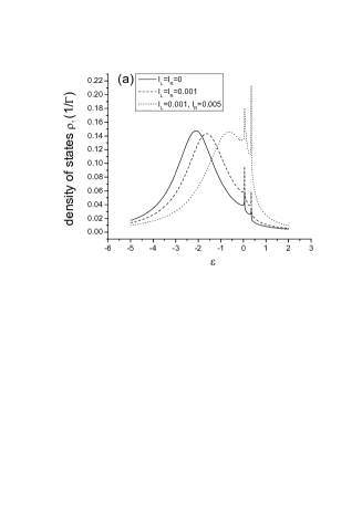
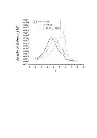
Figure 1: (a) and (b) are schematic diagrams of the density of states $\rho_{\sigma}(\epsilon)$ for a quantum dot symmetrically coupled to two leads with Lorentzian linewidth of $2D$. The quantum dot has two spin states with energies $\varepsilon_{\uparrow}=-2.9$, $\varepsilon_{\downarrow}=-3.1$ and an on-site interaction $U\rightarrow\infty$. The linewidth is chosen to be $D=500$ and the temperature is $T=0.005$. The spin bias is $V_{s}=0.3$ and the chemical potentials are $\mu_{L\uparrow}=-\mu_{L\downarrow}=V_{s}/2$ and $\mu_{R\downarrow}=-\mu_{R\uparrow}=V_{s}/2$. Solid, dashed and dotted curves correspond to interaction parameters of $I_{L}=I_{R}=0$, $I_{L}=I_{R}=0.001$ and $I_{L}=0.001,I_{R}=0.005$, respectively.

3 Numerical results

Having derived the nonequilibrium transport for the general case of a central region coupled to interacting leads, we investigate the spin transport through a quantum dot system with a spin bias $V_{s}$ applied at the two leads, namely $\mu_{L\uparrow}=-\mu_{L\downarrow}=V_{s}/2$ and $\mu_{R\downarrow}=-\mu_{R\uparrow}=V_{s}/2$. Our focus is to analyze the effect of the lead-dot Coulomb interaction on the spin-transport properties. Firstly, we start to study density of states of the quantum dot according to the relation $\rho_{\sigma}(\epsilon)=-(1/\pi)\mathrm{Im}G^{r}_{\sigma}(\epsilon)$. In the following numerical calculations, we assume that the quantum dot symmetrically couples to two leads with Lorentzian linewidth of $2D$, namely $\Gamma_{L\sigma}(\epsilon)=\Gamma_{R\sigma}(\epsilon)=\gamma_{0}D^{2}/2(\epsilon^{2}+D^{2})$, with $\gamma_{0}=1$ as the unit of energy and $D=500$. As for the dot-lead interaction, we adopt a flat-band profile, i.e., $I_{\alpha}(\epsilon)=I_{\alpha}\theta(D-|\epsilon|)$.

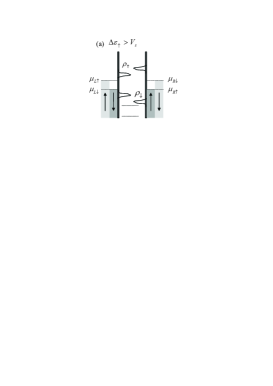
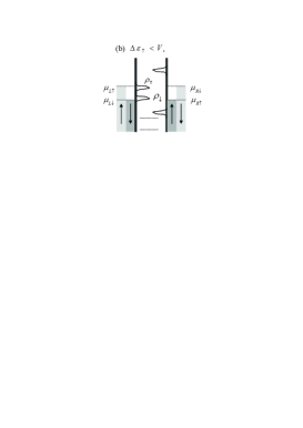
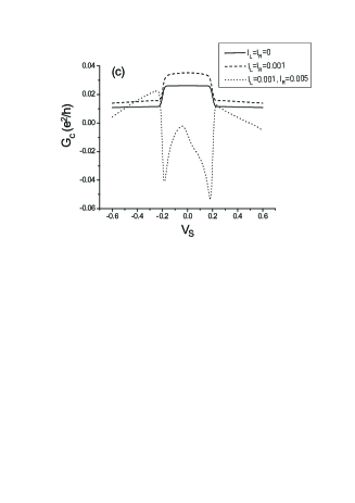
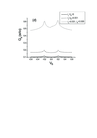
Figure 2: (a)-(b) Schematic energy diagrams of the Kondo density-of-state peaks and the electrochemical potentials of the two leads, for the case of $\Delta\varepsilon_{\uparrow}>V_{s}$ and $\Delta\varepsilon_{\uparrow}<V_{s}$. (c)-(d) The differential charge and spin conductance $G_{c}$ and $G_{s}$ plotted as a function of the spin bias $V_{s}$ for different lead-dot interaction strengths. Solid, dashed and dotted curves correspond to the case of $I_{L}=I_{R}=0$, $I_{L}=I_{R}=0.001$ and $I_{L}=0.001,I_{R}=0.005$, respectively. The energies of the quantum dot are chosen to be $\varepsilon_{\uparrow}=-2.9$, $\varepsilon_{\downarrow}=-3.1$, so that $\Delta\varepsilon_{\uparrow}=0.2$. Other parameters are the same as those of Figure 1.

As shown in Figure 1, the spin-up and spin-down density of states are plotted in the presence of dot-lead Coulombic interactions described by $I_{L}$ and $I_{R}$. In the absence of the dot-lead interaction, i.e., $I_{L}=I_{R}=0$ [solid line], a broad main peak is observed at $\epsilon\sim-2.5$, which is associated with the renormalized level $\varepsilon_{\uparrow}$ of the quantum dot. In addition, there are two sharp Kondo peaks at energies $\epsilon\approx 0$ and $\epsilon\approx 0.35$ [see Figure 1(a)]. The Kondo peaks for spin $\sigma$ arise from the contribution of the self-energy $\Sigma^{\prime}_{2\sigma}$, due to virtual intermediate states in which the site is occupied by an electron of opposite spin $\bar{\sigma}$ [3]. The real part of $\Sigma^{\prime}_{2\sigma}$ grows logarithmically near the energies $\epsilon_{\sigma}=\mu_{\alpha\bar{\sigma}}+\Delta\varepsilon_{\sigma}$ with $\Delta\varepsilon_{\sigma}=\varepsilon_{\sigma}-\varepsilon_{\bar{\sigma}}$, due to the sharp Fermi surface at low temperature. This logarithmic increase translates into peaks in the density of states near those energies. According to the same physical explanation, we can deduce that the Kondo peaks of the spin-down density of state $\rho_{\downarrow}$ should occur at energies $\epsilon=-0.05$ and $\epsilon=-0.35$, as can be confirmed from Figure 1(b). In the presence of the dot-lead interaction, for example $I_{L}=I_{R}=0.001$ (dashed lines), the position of the broad main peak is shifted. However, the positions of the Kondo peaks are not affected by the dot-lead interaction which induces the self-energies $\Sigma_{3\sigma}$ and $\Sigma_{4\sigma}$ and do not contribute to the Kondo effect. When the interaction strength is increased, e.g., $I_{R}=0.005$ (dotted line), the position of the broad main peak is shifted further to higher energy compared to the previous case, but the positions of the two Kondo peaks remain invariant.

Next, we investigate the effect of the dot-lead interaction on the charge and spin differential conductances, which are defined as $G_{c}=dJ/dV_{s}$ and $G_{s}=dJ_{s}/dV_{s}$, where $J_{s}=\hbar(J_{\uparrow}-J_{\downarrow})/2e$, respectively. The differential conductance $G_{c}$ and $G_{s}$ are plotted as a function of the spin bias $V_{s}$ for different interaction strengths as shown in Figure 2. To explain the observed trends in the spin and charge differential conductance, we sketch the electrochemical potentials in the two leads, and superimpose on it the Kondo peaks in the density-of-states [see Figs. 2(a) and (b)]. We observe a plateau in $G_{c}$ over the bias interval of $|V_{s}|\leq 0.2$, for the cases of $I_{L}=I_{R}=0$ and $I_{L}=I_{R}=0.001$. However, the conductance plateau is destroyed in the case of asymmetric lead-dot interaction, i.e. $I_{L}\neq I_{R}$, and the charge differential conductance assumes a negative value over the same bias interval [see Figure 2(c)]. The spin differential conductance $G_{s}$ shows two Kondo peaks at $|V_{s}|=0.2$, irrespective of the symmetry or strength of the lead-dot interactions [shown in Figure 2(d)]. $G_{s}$ is also enhanced with increasing strength of the dot-lead interactions.

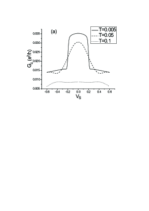
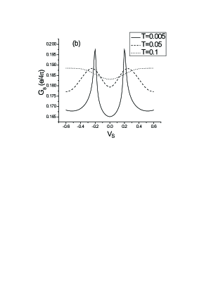
Figure 3: The differential charge and spin conductance $G_{c}$ (a) and $G_{s}$ (b) versus the spin bias $V_{s}$, for temperatures $T=0.005$ (solid line), $T=0.05$ (dashed line) and $T=0.1$ (dotted line). The lead-dot interaction strength is set at $I_{L}=I_{R}=0.001$. Other parameters are the same as those of Figure 1.

We note that the spin-up and spin-down electrons flow along opposite directions, i.e., $J=|J_{\uparrow}|-|J_{\downarrow}|$ and $J_{s}\propto|J_{\uparrow}|+|J_{\downarrow}|$, and that the two currents $J_{\uparrow}$ and $J_{\downarrow}$ can be different due to the energy splitting $\Delta\varepsilon_{\uparrow}$. To explain the above conductance dependence on $V_{s}$, we refer to the schematic diagram of the Kondo density-of-state peaks [see Figure 2(a)-(b)]. The Kondo peaks begin to enter the spin-bias conduction window when the spin bias is increased beyond $|V_{s}|=\Delta\varepsilon_{\uparrow}$. This results in the spin differential conductance $G_{s}$ having two Kondo peaks at $V_{s}=\pm\Delta\varepsilon_{\uparrow}$. The entry of the two Kondo peaks into the conduction window also reduces the difference in the magnitude of $J_{\uparrow}$ and $J_{\downarrow}$, thus resulting in a sharp drop (plateau step) in the charge conductance at $V_{s}=\pm\Delta\varepsilon_{\uparrow}$. The conductance plateau can thus be attributed to the combined effect of the spin bias in the leads and the Zeeman splitting in the QD. The dot-lead interaction tends to increase the coupling between the leads and the QD, thus resulting in a general increase in the charge and spin differential conductances. In the presence of asymmetrical dot-lead interaction, i.e., $I_{L}=0.001$ and $I_{R}=0.005$, the symmetry in the transport across the QD is broken, and thus the conductance plateau disappears. Two conductance dips occur at $|V_{s}|<\Delta\varepsilon_{\uparrow}$ due to the contribution from the Kondo peaks in the density-of-states.

Finally we study the temperature dependence of the differential conductances. As shown in Figure 3, the two Kondo peaks in $G_{s}$ at $V_{s}=\pm 0.2$, and the conductance plateau in $G_{c}$ in the bias interval $|V_{s}|<0.2$ can be clearly observed at a low temperature of $T=0.005$. With increasing temperature, e.g., at $T=0.05$, the Kondo peaks become thermally broadened, while the plateau in $G_{c}$ sharpens into a peak profile. With a further increase in temperature to $T=0.1$, the plateau in $G_{c}$ is almost completely suppressed. These changes can be largely attributed to the thermal distribution of electrons about the electrochemical potential in the leads. The thermal distribution in turn affects the self-energy $\Sigma_{2\sigma}^{\prime}$ of the intra-dot Coulomb interaction, which is primarily responsible for the Kondo resonances in the density-of-states [see Eq. (27)].

4 Summary

In this work, we analyze the spin-transport properties of a quantum dot system driven by spin bias in the presence of dot-lead Coulombic interactions. The transport property is discussed on the basis of Keldysh nonequilibrium Green’s function framework. According to the equation-of-motion technique and Langreth’s theorem, we derive the analytical expression of the current through the quantum dot in the presence of the dot-lead Coulombic interaction. Our numerical results show that although the interaction can renormalize the energy levels of the quantum dot, they leave the position of the Kondo peaks in the density of states unchanged. This is because the Kondo effect arises primarily for intra-dot Coulomb interactions involving electrons of opposite spins. The Kondo resonances in the density of states translate into peaks in the spin differential conductance when the magnitude of the spin bias is equal to that of the Zeeman energy split in the quantum dot. There also exists a plateau in the charge differential conductance at low bias, due to the combined effect of spin bias and the Zeeman energy splitting. The position of the steps of the conductance plateau can also be attributed to the Kondo effect. The strength of the Coulombic lead-dot interactions affects the magnitude of both the spin and charge conductances. Furthermore, in the presence of asymmetrical dot-lead interaction strengths, the plateau in the charge conductance disappears, and is replaced by conductance peaks. Finally, the temperature dependence of the differential conductances is qualitatively discussed.

The authors would like to thank the Agency for Science, Technology and Research (A*STAR) of Singapore, the National University of Singapore (NUS) Grant No. R-398-000-061-305 and the NUS Nanoscience and Nanotechnology Initiative for financially supporting their work. The work was also supported by Innovation Research Team for Spintronic Materials and Devices of Zhejiang Province.

References

[1]
T. K. Ng and P. A. Lee, Phys. Rev. Lett. 61, (1988) 1768; S.
Hershfield, J. H. Davies and J. W. Wilkins, Phys. Rev. Lett.
67, (1991) 3720.
[2]
L. I. Glazman and M. E. Raikh, JETP Lett., 47 (1988) 378.
[3]
Y. Meir, N. S. Wingreen and P. A. Lee, Phys. Rev. Lett. 70
(1993) 2601.
[4]
M. Pustilnik and L. I. Glazman, Phys. Rev. Lett. 87 (2001)
216601.
[5]
Q. F. Sun and H. Guo, Phys. Rev. B 66 (2002) 155308.
[6]
J. Martinek, Y. Utsumi, H. Imamura, J. Barnaś, S. Maekawa, J.
König, and G. Schön, Phys. Rev. Lett. 91(2003) 127203.
[7]
D. Goldhaber-Gordon, J. Göres, M. A. Kastner, H. Shtrikman, D.
Mahalu, and U. Meirav, Phys. Rev. Lett. 81 (1998) 5225.
[8]
S. Sasaki, S. De Franceschi, J. M. Elzerman, W. G. van der Wiel, M.
Eto , S. Tarucha, L. P. Kouwenhoven, Nature (London) 405 (2000)
764.
[9]
N. Sergueev, Q. F. Sun, H. Guo, B. G. Wang, and J. Wang, Phys. Rev.
B 65 (2002) 165303.
[10]
P. Zhang, Q. K. Xue, Y. P. Wang, and X. C. Xie, Phys. Rev. Lett.
89 (2002) 286803.
[11]
A. N. Pasupathy, R. C. Bialczak, J. Martinek, J. E. Grose, L. A. K.
Donev, P. L. Mceuen, and D. C. Ralph, Science, 306 (2004) 86.
[12]
Y. Utsumi, J. Martinek, G. Schön, H. Imamura, and S. Maekawa,
Phys. Rev. B 71 (2005) 245116.
[13]
E. J. Koop, B. J. van Wees, D. Reuter, A. D. Wieck, and C. H. van
der Wal, Phys. Rev. Lett. 101 (2008) 056602.
[14]
Y. K. Kato, R. C. Myers, A. C. Gossard, D. D. Awschalom, Science
306 (2004) 1910.
[15]
S. O. Valenzuela, M. Tinkham, Nature (London) 442 (2006) 176.
[16]
Y. J. Bao, N. H. Tong, Q. F. Sun, and S. Q. Shen, Europhys. Lett.
83, (2008) 37007.
[17]
R. Świrkovicz, J. Barnaś, and M. Wilczyński, J. Magn.
Magn. Mater. 321 (2009) 2414.
[18]
T. Kobayashi, S. Tsuruta, S. Sasaki, T. Fujisawa, Y. Tokura, and T.
Akazaki, Phys. Rev. Lett. 104 (2010) 036804.
[19]
Y. Meir and N. S. Wingreen, Phys. Rev. Lett. 68 (1992) 2512.
[20]
A. P. Jauho, N. S. Wingreen, and Y. Meir, Phys. Rev. B 50
(1994) 5528.
[21]
M. Buongiorno Nardelli, Phys. Rev. B 60 (1999) 7828.
[22]
Q. F. Sun, J. Wang, and H. Guo, Phys. Rev. B 71 (2005) 165310.
[23]
T. C. Li and S. P. Lu, Phys. Rev. B 77 (2008) 085408.
[24]
S. Bala Kumar, M. B. A. Jalil, S. G. Tan, and G. C. Liang, J. Appl.
Phys. 108 (2010) 033709.
[25]
M. Sade, Y. Weiss, M. Goldstein, and R. Berkovits, Phys. Rev. B
71 (2005) 153301.
[26]
Y. Meir, N. S. Wingreen, and P. A. Lee, Phys. Rev. Lett. 66
(1991) 3048.
[27]
H. Huag and A. P. Jauho 1998 Quantum Kinetics in transport and
optics of semiconductors, Springer serier in solid-state sciences,
edited by Cardona M, Fulde P, von Klitzing K and Queisser H J.