Link Prediction in Complex Networks: A Clustering Perspective

Abstract

Link prediction is an open problem in the complex network, which attracts much research interest currently. However, little attention has been paid to the relation between network structure and the performance of prediction methods. In order to fill this vital gap, we try to understand how the network structure affects the performance of link prediction methods in the view of clustering. Our experiments on both synthetic and real-world networks show that as the clustering grows, the precision of these methods could be improved remarkably, while for the sparse and weakly clustered network, they perform poorly. We explain this through the distinguishment caused by increased clustering between the score distribution of positive and negative instances. Our finding also sheds light on the problem of how to select appropriate approaches for different networks with various densities and clusterings.

1 Introduction

Many real world data sets can be represented as networks with nodes denoting objects and edges describing relationships between them Survey . Examples of complex networks include the Internet, a collection of connected Autonomous Systems(AS), routers and interfaces in different levels. The online social network for people maintaining their friendship is another major instance. For the pervasive existence of these networks, the last decade has witnessed the study of complex networks in the fields of both computer science and physics. An important issue relevant to the computational analysis of complex networks is the link prediction. Link prediction is a problem of both theoretical and practical significance. It aims to evaluate the likelihood of a link between two nodes not connected until now, based on the existing links information and possible node attributes information in the network physica . There are two aspects of link prediction problem: on the one hand, for most real network data, not all links are already observed, link prediction helps to find the missing links; on the other hand, it can help us infer the new interactions between nodes in the new future. Research on link prediction is also helpful to accomplish some other tasks, like collective classification CCLP and anomalous link discovery ALD .

The existing methods for link prediction can be divided into three categories. The first method defines a measure of proximity or similarity between two nodes in the network, taking into account that links between more similar nodes are of higher existing likelihood. Liben-Nowell and Kleinberg Nowell summarize many similarity measures based on node neighborhoods, the ensemble of all paths and higher-level approaches. They compare these measures with random predictors in five co-authorship networks and find that there is indeed useful information contained in the network topology alone. Motivated by the resource allocation process taking place in networks, Zhou et al. RA propose a new similarity measure, which has great performance in six representative networks drawn from different fields. Liu and Lü SRW put forward a method based on local random walk, which can give excellent prediction while has low computational complexity. The second method is based on the maximum likelihood estimation. Empirical studies suggest that many real-world networks exhibit hierarchical organization. Clauset, Moore and Newman Nature present a method inferring hierarchical structure from network data and use the knowledge of hierarchical structure to predict the missing links in partially known networks. The third method mainly uses machine learning techniques. Hasan et al Supervised_Learning view link prediction as a supervised learning task: for two potentially connected nodes, predicting whether it is a positive or negative example. The feature set extracted from the co-authorship graph contains proximity features, aggregated features and topological features. They experiment with seven different classification algorithms and compare the performance of these classifiers using different performance metrics. O’Madadhain et al. Event_network use primarily probabilistic classifiers to predict future “co-participating” in event-based network data. There are also many works related to link prediction concerning more complicated networks, like directed and weighted networks. Leung et al. LFR propose a novel Link Formation Rules mining algorithm for social networks. Romero and Kleinberg Closure investigate the directed closure process and analyze the link formation on twitter. In weight_network , Murata and Moriyasu describe an improved method for predicting links on Question-Answering Bulletin Boards (QABB), kind of a social network in which each link is assigned a weight.

Most of those works on link prediction aim to find a method with better prediction performance for some particular networks, such as the co-authorship network, terrorists network and so on. However, little was done to reveal how these existing methods perform on networks with different structural properties. In this paper, we try to find the relation between network structure and the prediction performance of these methods. In the real world, the attributes of nodes are usually difficult to collect and the simpleness of prediction methods is also necessary. For example, in online social networks, systems need to provide a list of potential friends for a certain user with least load to the server. Because of this, in the present work, we focus on the first kind of methods which are solely based on the network structure. Through experiments on both synthetic and real-world networks, we find that for the network with low clustering, these methods perform poorly. Nonetheless, as the clustering of the network grows, the precision of these methods is drastically improved. These phenomena tell us that for the networks with various clusterings, we should employ different methods for link prediction.

This rest of the present paper is organized as follows: In Section 2, we review several similarity based methods for link prediction. In Section 3, the data sets we use in the paper are introduced. We investigate the connection between clustering and performance of prediction methods in Section 4, and we also give a brief explanation in this section. In Section 5, we conclude this work briefly.

2 Preliminaries

In this section, we first describe the link prediction problem and introduce the evaluation metrics. Then we review several similarity-based methods.

Suppose we have an undirected simple network $G(V,E)$, where $V$ is the set of nodes and $E$ is the set of edges. Generally, the number of a node’s connections can be defined as its degree. The averaged degree of the network can be defined as

$$\langle k\rangle=\frac{2|E|}{|V|},$$

which could be used to characterize the density of the network. We use $p(k)$ to denote the degree distribution of the network and for the complex networks discussed in this paper, it always follows a power-law. The relative size of the giant connected component($GCC$) can be denoted as $f_{GCC}.$ Clustering of a node $i$ is used to characterize how closely its neighbors are connected. It can be defined as

$$C_{i}=\frac{2|E_{i}|}{k_{i}(k_{i}-1)},$$

where $E_{i}$ is the set of ties between $i$’s neighbors and $k_{i}$ is the degree of $i$. We do not take the case of $k_{i}=1$ into consideration. The averaged clustering of the network can be defined as

$$C=\frac{\sum_{\{i\in V\}}{C_{i}}}{|V|}.$$ (1)

In the rest of paper, we omit the word “averaged” if there is no confusion in the context.

For any pair of nodes $\langle x,y\rangle$, which is not existing in $E$, each similarity-based method defines a measure, i.e. a score $s(x,y)$ is assigned according to the given network topology. Then we rank all of these scores of node pairs and a higher score means a higher probability that the corresponding link will emerge in the future or more likely be missed in the present sample.

To test the prediction accuracy of each method, we adopt the approach used in RA . The edge set $E$ is randomly divided into two parts, including $E^{Train}$ and $E^{Test}$, respectively. The training set $E^{Train}$ is supposed to be known information and $E^{Test}$ is the testing set consisting of missing links or links to occur in the future. The training set contains 90% of links in $E$, and the remaining 10% of links are in the testing set. We use precision to quantify the accuracy of prediction measures, which is determined as follows. Let $n$ denote the number of links in $E^{Test}$. We compute the score list based on $G(V,E^{Train})$ and rank the list in decreasing order. The first $n$ pairs are taken and $m$ denotes the size of the intersection of this set of pairs with the $E^{Test}$. Then the precision is $P=m/n$.

We mainly explore six existing similarity-based measures for link prediction, including (1) Common Neighbors(CN); (2) Adamic-Adar Index(AA); (3) Resource Allocation Index(RA); (4) Katz Index(Katz); (5) Rooted PageRank(PR); (6) Superposed Random Walk(SRW). A brief introduction of these methods is given as follows.

Common Neighbors For a node $x$ in $G$, $N(x)$ denotes the set of neighbors of $x$. The Common Neighbors measure is determined by the number of nodes that link to both $x$ and $y$, that is to say, two nodes is more likely to be connected with more common neighbors. Therefore, the score can be defined as

$$s^{CN}(x,y)=|N(x)\cap N(y)|.$$ (2)

Adamic-Adar Index In AA , to determine whether two personal home pages are strongly “related”, Adamic and Adar define the similarity between two pages based on their shared features. For link prediction, this index assigns rarer connected node more weights, i.e.,

$$s^{AA}(x,y)=\sum_{z\in N(x)\cap N(y)}{1/log(k(z))},$$ (3)

where $k(z)$ is the degree of the node $z$.

Resource Allocation Index Zhou et al. RA consider such a process: for a pair of unconnected nodes $x$ and $y$, $x$ with a unit of resource can send some to $y$ by sending averaged amounts to its neighbors. The more resource $y$ receives from $x$, the more likely a link between $x$ and $y$ exists. Therefore, the score between x and y is defined as

$$s^{RA}(x,y)=\sum_{z\in N(x)\cap N(y)}{1/k(z)}.$$ (4)

Katz Index Katz Index is a path-ensemble based method. It sums over all paths between $x$ and $y$. The more number of paths with short length, the higher the score is. It is defined as

$$s^{Katz}(x,y)=\sum_{l=1}^{\infty}{\beta^{l}\cdot|paths^{l}_{x,y}|},$$ (5)

where $\beta$ is an adjusting parameter and $paths^{l}_{x,y}$ is the set of all paths with length $l$ from $x$ to $y$. As mentioned in  Nowell , we can get the score matrix $S^{Katz}$ by

$$S^{Katz}=\sum_{l=1}^{\infty}{\beta^{l}A^{l}}=(I-\beta A)^{-1}-I,$$ (6)

where $I$ is the identity matrix and $A$ is the adjacent matrix of $G$.

Rooted PageRank Index The Rooted PageRank defines a random walk on the underlying graph $G$. A random walk starts from a node $x$, and iteratively moves to a neighbor of $x$ chosen uniformly at random. We use the probability that a random walk starting from $x$ runs into $y$ as the indicator of similarity between $x$ and $y$ imc . The $s^{PR}(x,y)$ under the Rooted PageRank is defined to be the stationary probability of $y$ under such a random walk: with probability $1-\beta$ returns to $x$ at each step, moves to a random neighbor of the current node with probability $\beta$. Let

$$D_{ii}=1/\sum{A_{ij}},$$

$D_{ij}=0$ when $i\neq j$ and

$$T=DA,$$

we have the score matrix $S^{PR}$

$$S^{PR}=(1-\beta)(I-\beta T)^{-1}.$$ (7)

Superposed Random Walk Liu and Lü SRW propose the Superposed Random Walk Index, which focuses on just few-step random walk, rather than the stationary probability. The transition probability matrix is denoted as $P$, with $P_{xy}=a_{xy}/k_{x},$ where $a_{xy}$ represents the corresponding entry in $A$. Given a random walk starting at $x$, the probability that it locates at $y$ after $t$ steps is $\pi_{xy}(t)$. $\overrightarrow{\pi}_{x}(0)$ is a $N*1$ vector with $x^{th}$ element equals 1 and others equal 0. Then we have:

$$\overrightarrow{\pi}_{x}(t)=P^{T}\overrightarrow{\pi}_{x}(t-1).$$ (8)

The similarity based on Local Random Walk is defined as:

$$s^{LRW}_{xy}(t)=\frac{k_{x}}{2|E|}\cdot\pi_{xy}(t)+\frac{k_{y}}{2|E|}\cdot\pi_{yx}(t).$$ (9)

The Superposed Random Walk Index superposes the contribution of independently moved walkers and in our configuration we compute the 3 steps SRW rather than the optimal-steps SRW. The score for the pair $\langle x,y\rangle$ can be defined as

$$s^{SRW}(x,y,t)=\sum_{\tau=1}^{t}{s_{xy}^{LRW}(\tau)}.$$ (10)

Through the measure of precision and these prediction methods, we then perform experiments on both the synthetic and real-world networks that will be introduced in the next section.

3 Data Sets

The complex networks are pervasively existing in the real-world. Empirical study suggests that most complex networks exhibit the “scale-free” property, which means $p(k)\propto k^{-\gamma}$. Barabási and Albert BA proposed a scale-free network model to explain the generation mechanism of the “power-law” distribution, known as the BA model. We utilize this model to generate the synthetic networks. We denote the network generated by the BA model as $BA(N,m)$, where $N$ is the size of the network generated, $m$ is the number of links that a new node will establish when it is added to the network and the averaged degree is $2m$. We generate five networks in this paper.

We also import three typical real-world complex networks collected from different fields. Netscience is a network of co-authorships between scientists who are themselves publishing on the topic of network science netscience . There are 1589 scientists in this network and 128 of them are isolated. We will not use these isolated nodes in our experiment. Power Grid is a well-connected electrical power grid of western US, where nodes denote generators, transformers and substations and edges denote the transmission lines between them Grid . Politic Blog is a directed network of US political blogs PB . Here we treat its links as undirected and self-connections are omitted.

The detailed descriptions of these data sets are listed in Table 1.

Table 1: Synthetic and real-world data sets

Network	$|V|$	$|E|$	$\langle k\rangle$	$C$	$f_{GCC}$
BA(1000,2)	1000	1997	4	0.027	1
BA(1000,5)	1000	4985	10	0.039	1
BA(1000,10)	1000	9945	20	0.064	1
BA(2000,5)	2000	9985	10	0.024	1
BA(4000,5)	4000	19985	10	0.017	1
Netscience	1461	2742	3.75	0.878	0.26
Power Grid	4941	6594	2.67	0.107	1
Politic Blog	1224	16715	27.31	0.36	0.998

4 How Clustering affects Predicting Precision

In this section, we first perform experiments on synthetic networks with various clusterings and unveil the relation between the network structure and the precision of link prediction methods. Then we validate our findings on the representative real-world data sets. Finally, we give an explanation based on class distribution for the phenomenon.

4.1 Results from Synthetic Networks

We investigate the relationship between the clustering and the precision of link prediction in this subsection. In order to unveil this relationship, the variation of clustering of the network is necessary. For this reason, we use the method proposed by Kim et al. kim_clustering to rewire the links randomly and achieve the purpose of varying the clustering but without changing the degrees of the nodes. In particular, we first randomly pick up two edges, say $\langle A,B\rangle$ and $\langle C,D\rangle$. We then compare the numbers of local triangular structures associated with all three configurations $\{\langle A,B\rangle,\langle C,D\rangle\}$, $\{\langle A,C\rangle,\langle B,D\rangle\}$ and $\{\langle A,D\rangle,\langle B,C\rangle\}$, and select the one with most triangles and connect the nodes accordingly, where duplicated links are avoided ma_clustering . It is worthy to note that, in this process, if a link from a given node is detached, a different link is immediately attached to this node. We continue this process until a desirable value of $C$ of the network is attained. In this approach, the degree sequence of the network are fixed, and the only topological property changed is $C$.

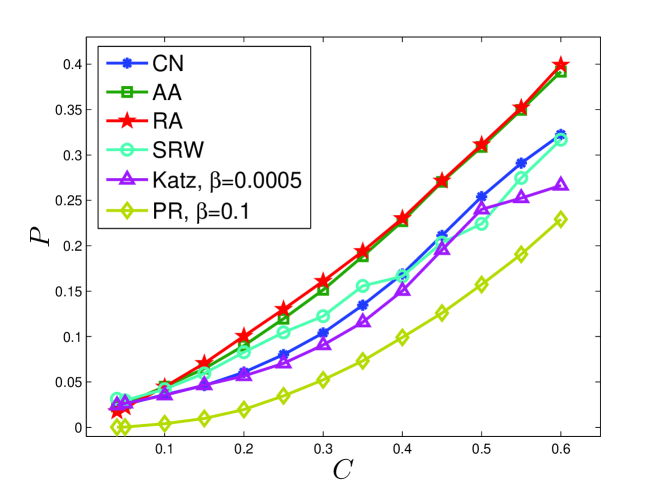
Figure 1: Link prediction on BA(1000,5) with varying clustering

Table 2: The result from BA(4000,5)

$C$	CN	AA	RA	SRW	Katz			PR
					$\beta=0.05$	$\beta=0.005$	$\beta=0.0005$	$\beta=0.1$	$\beta=0.5$	$\beta=0.9$
0.0176	0.0134	0.0128	0.0096	0.0145	0.0003	0.0134	0.0150	9.91E-05	5.04E-05	0.0012
0.1	0.0393	0.0595	0.0541	0.0509	0.0159	0.0318	0.0305	0.0046	0.0038	0.0051
0.15	0.0557	0.0901	0.0846	0.0704	0.0321	0.0404	0.0383	0.0091	0.0095	0.0105
0.2	0.0722	0.1189	0.1159	0.0932	0.0487	0.0534	0.0544	0.0205	0.0183	0.0185
0.25	0.0925	0.1461	0.1430	0.1132	0.0592	0.0638	0.0657	0.0358	0.0334	0.0326
0.3	0.1168	0.1781	0.1726	0.1342	0.0616	0.0832	0.0800	0.0522	0.0532	0.0501
0.35	0.1432	0.2130	0.2037	0.1610	0.0937	0.1054	0.1067	0.0744	0.0702	0.0690
0.4	0.1785	0.2514	0.2405	0.1827	0.1060	0.1383	0.1410	0.0979	0.0943	0.0898
0.45	0.2162	0.2898	0.2774	0.2140	0.1203	0.1790	0.1841	0.1184	0.1184	0.1104
0.5	0.2573	0.3279	0.3163	0.2458	0.1320	0.2391	0.2346	0.1541	0.1519	0.1364
0.55	0.3074	0.3704	0.3616	0.2824	0.1152	0.2983	0.3025	0.1882	0.1853	0.1702
0.6	0.3450	0.4132	0.4081	0.3154	0.1241	0.3226	0.3292	0.2267	0.2143	0.1903

We perform the six methods on different generated networks with various clusterings. The results from BA(1000,5) are shown in Fig. 1. As for Katz and PR, we only choose the best situation to represent them, i.e. $\beta=0.0005$ for Katz and $\beta=0.1$ for PR. It can be seen that while the clustering $C$ increases, all these similarity-based methods have better prediction performance. In networks with relatively small $C$, e.g. $C<0.01$, there doesn’t exist a more competitive method, and while $C$ grows to a certain value, AA and RA seem to be better. The results from other synthetic data sets are similar. For example, Table 2 shows the result from BA(4000,5). We can see that the correlated characteristic between $C$ and prediction value of different methods does not vary with the size and density of the network. It is also interesting that for the method of Katz, its performance depends on the value of $\beta$ greatly. For instance, when $\beta=0.0005$, it performs best as clustering grows. This phenomenon means that the nearest neighbors play a vital role in the prediction for Katz, however, considering the further hops is unnecessary.

Meanwhile, as shown in Fig. 2, we choose three representative clusterings, i.e., $C=0.1$, $C=0.3$ and $C=0.5$, to observe how these methods perform on networks with different densities when the size and clustering of the networks are constant. It is easy to learn from Fig. 2 that these methods perform better on denser networks. However, for the sparse network with low clustering, say $C=0.1$, as shown in Fig. 2(a), SRW performs best compared with other approaches when $m=2$. Nevertheless, the situation changes when the clustering of the network grows, AA and RA perform better, too. In particular, RA is the best way among these methods for the dense network with high clustering, as shown in Fig. 2(c).

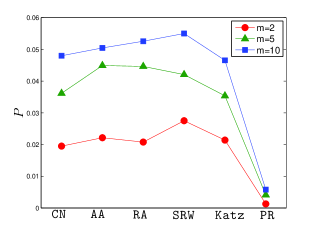
(a) $C=0.1$

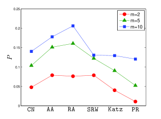
(b) $C=0.3$

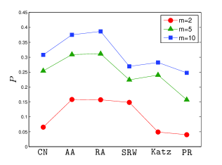
(c) $C=0.5$

Figure 2: $P$ varies with density of the network

In summary, we find that on the synthetic networks generated by BA model, when the clustering grows, the performance of these prediction methods improves. However, a natural question is whether similar phenomenon can be found in real-world networks. Therefore, we validate this finding on the real-world data sets in the next subsection.

4.2 Validation on Real-world Data Sets

The result of link prediction experiments on these real-world networks is shown in Table 3, which is consistent with the above simulation experiment. We can see that the prediction methods perform best on Netscience which has the largest clustering and worst on Power Grid with the least $C$.

Table 3: The result from real-world data sets

Network	CN	AA	RA	SRW	Katz			PR
					$\beta=0.05$	$\beta=0.005$	$\beta=0.0005$	$\beta=0.1$	$\beta=0.5$	$\beta=0.9$
Netscience	0.4494	0.6666	0.6805	0.5760	0.3796	0.4569	0.4423	0.3734	0.3817	0.3013
Power Grid	0.0438	0.0281	0.0252	0.0227	0.0085	0.0067	0.0110	0.0085	0.0067	0.0110
Politic Blog	0.1724	0.1712	0.1497	0.1421	0.0309	0.1776	0.1733	0.0141	0.0288	0.0537

Based on the validations above, we can conjecture that in real-world networks, the performance of these link prediction methods is closely related to their clusterings. That is, for the network with higher clustering, these methods perform better. However, when the clustering decreases, their precision drops.

4.3 An Explanation Based on Class Distribution

In this subsection, we try to explain the finding in the view of class distribution. Here we treat the pair of connected nodes as a positive instance while the pair of disconnected nodes is a negative instance. As mentioned in ALD , the highly skewed distribution of positive and negative examples yields computational cost of all node pairs and increases the variance of the prediction model. We assume that the scores of each particular link prediction method are drawn from separate distributions for linked and non-linked node pairs. In principle, the similarity-based method for link prediction tries to distinguish the two distributions of positive and negative examples by the corresponding scores. Next, we focus on how the distribution of scores on two types of node pairs varies as the network structure changes.

As shown in Fig. 3(a), Fig. 3(b) and Fig. 3(c), for CN, we can see a clear separation between the distributions of $s^{CN}$ on positive and negative pairs while $C$ of the network increases from 0.039 to 0.5. This trend can also be observed with RA, as shown in Fig. 3(d), Fig. 3(e), and Fig. 3(f). As clustering of the network increases, node pairs with higher scores are more likely positive instances. Remember that in the link prediction process, a higher score means a higher probability that a link will emerge or more likely be missed, so we can conclude that these prediction methods are more effective in networks with greater clusterings. In summary, the increment of clustering improves the capability of these methods for distinguishing the positive and negative node pairs, which leads to a higher prediction precision as the experiment shows.

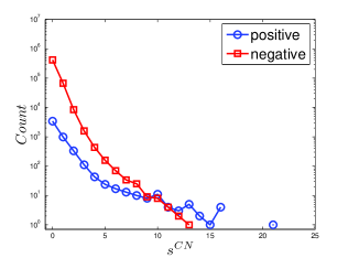
(a) CN, $C=0.039$

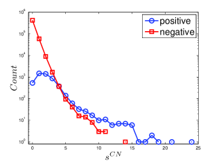
(b) CN, $C=0.3$

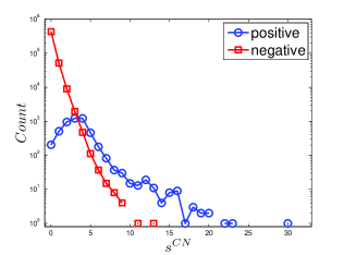
(c) CN, $C=0.5,$

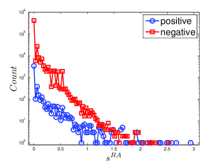
(d) RA, $C=0.039$

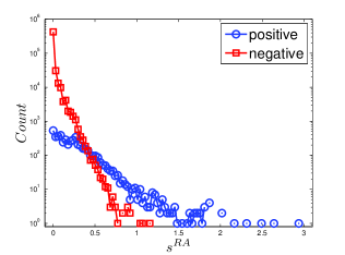
(e) RA, $C=0.3$

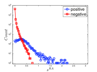
(f) RA, $C=0.5$

Figure 3: Relative distribution of scores for positive and negative instances as $C$ increases.

5 Conclusion

Link prediction is an open problem in the complex network, which attracts wide attention in recent years. Plenty of methods have been presented, some of which are solely based on the structure while some of which take other features of the network into account. However, in the real-world, the simpleness and freedom of need for rich attributes are necessary to the practical methods. For this reason, we mainly investigate the relationship between six structural approaches and the clustering of networks. It is interesting that we find the performance of these methods improves tremendously as the clustering increases both on synthetic and real-world networks. We also give this a brief explanation through the extent of distinguishment between the distribution of positive and negative instances caused by the variation of clustering. Our finding also sheds light on the problem of how to choose a simple but effective method when we meet real networks with various clusterings. We conjecture that for the sparse network with lower clustering, SRW is the best choice, while for the network which is dense and highly clustered, the best choice is RA.

6 Acknowledgement

This work was supported by the fund of the State Key Laboratory of Software Development Environment (SKLSDE-2008ZX-03).

References

- (1) R. Ackland. Mapping the us political blogosphere: Are conservative bloggers more prominent? Presentation to Blog Talk Downunder, 2005.
- (2) L. A. Adamic and E. Adar. Friends and neighbors on the web. SOCIAL NETWORKS, 25:211–230, 2001.
- (3) A.-L. Barabasi and R. Albert. Emergence of scaling in random networks. SCIENCE, 286:509, 1999.
- (4) M. Bilgic, G. M. Namata, and L. Getoor. Combining collective classification and link prediction. In Proceedings of the Seventh IEEE International Conference on Data Mining Workshops, ICDMW ’07, pages 381–386, Washington, DC, USA, 2007. IEEE Computer Society.
- (5) A. Clauset, C. Moore, and M. E. J. Newman. Hierarchical structure and the prediction of missing links in networks. Nature, 453:98–101, 2008.
- (6) L. Getoor and C. P. Diehl. Link mining: a survey. SIGKDD Explor. Newsl., 7:3–12, December 2005.
- (7) M. A. Hasan, V. Chaoji, S. Salem, and M. Zaki. Link prediction using supervised learning. In Proc. of SDM 06 workshop on Link Analysis, Counterterrorism and Security, 2006.
- (8) B. J. Kim. Performance of networks of artificial neurons: The role of clustering. Phys. Rev. E, 69(4):045101, Apr 2004.
- (9) C. W.-k. Leung, E.-P. Lim, D. Lo, and J. Weng. Mining interesting link formation rules in social networks. In Proceedings of the 19th ACM international conference on Information and knowledge management, CIKM ’10, pages 209–218, New York, NY, USA, 2010. ACM.
- (10) D. Liben-Nowell and J. Kleinberg. The link prediction problem for social networks. In Proceedings of the twelfth international conference on Information and knowledge management, CIKM ’03, pages 556–559, New York, NY, USA, 2003. ACM.
- (11) W. Liu and L. Lü. Link prediction based on local random walk. EPL, 89, 2010.
- (12) L. Lü and T. Zhou. Link prediction in complex networks: A survey. Physica A, 390:1150–1170, 2011.
- (13) X. Ma, L. Huang, Y.-C. Lai, and Z. Zheng. Emergence of loop structure in scale-free networks and dynamical consequences. Phys. Rev. E, 79(5):056106, May 2009.
- (14) T. Murata and S. Moriyasu. Link prediction of social networks based on weighted proximity measures. In Proceedings of the IEEE/WIC/ACM International Conference on Web Intelligence, WI ’07, pages 85–88, Washington, DC, USA, 2007. IEEE Computer Society.
- (15) M. E. J. Newman. Finding community structure in networks using the eigenvectors of matrices. Phys. Rev. E, 74(3):036104, Sep 2006.
- (16) J. O’Madadhain, J. Hutchins, and P. Smyth. Prediction and ranking algorithms for event-based network data. SIGKDD Explor. Newsl., 7:23–30, December 2005.
- (17) M. J. Rattigan and D. Jensen. The case for anomalous link discovery. SIGKDD Explor. Newsl., 7:41–47, December 2005.
- (18) D. Romero and J. Kleinberg. The directed closure process in hybrid social-information networks, with an analysis of link formation on twitter. In International AAAI Conference on Weblogs and Social Media, 2010.
- (19) H. H. Song, T. W. Cho, V. Dave, Y. Zhang, and L. Qiu. Scalable proximity estimation and link prediction in online social networks. In Proceedings of the 9th ACM SIGCOMM conference on Internet measurement conference, IMC ’09, pages 322–335, New York, NY, USA, 2009. ACM.
- (20) D. J. Watts and S. H. Strogatz. Collective dynamics of ‘small-world’ networks. Nature, 393:440–442, 1998.
- (21) T. Zhou, L. Lü, and Y.-C. Zhang. Predicting missing links via local information. Eur. Phys. J. B, 71:623–630, 2009.