Dispersive representation of the scalar and vector K$\pi$ form factors for $\tau\rightarrow K\pi\nu_{\tau}$ and $K_{\ell 3}$ decays

Abstract

Recently, the $\tau\rightarrow K\pi\nu_{\tau}$ decay spectrum has been measured by the Belle and BaBar collaborations. In this work, we present an analysis of such decays introducing a dispersive parametrization for the vector and scalar K$\pi$ form factors. This allows for precise tests of the Standard Model. For instance, the determination of $f_{+}(0)|V_{us}|$ from these decays is discussed. A comparison and a combination of these results with the analyses of the $K_{\ell 3}$ decays is also considered.

1 INTRODUCTION

Despite the great success of the Standard Model (SM), there are indications that it is the effective theory of a more fundamental theory with new degrees of freedom appearing at the TeV scale. There exist two main approaches to look for physics beyond the Standard Model: direct searches for new particles (Charged Higgs, Supersymmetric particles, Z’, W’…) at high ener-gy colliders and indirect searches, for instance in flavour physics, through precision experiments.

We will follow here the second approach and test the SM studying the $\tau\rightarrow K\pi\nu_{\tau}$ and $K_{\ell 3}$ decays. For that a very precise knowledge of the K$\pi$ form factors is necessary. Until recently, experimental information on these form factors was only coming from the $K_{\ell 3}$ ($K\rightarrow\pi\ell\nu_{\ell}$, $\ell=\mu,e$) decay measurements [1]. But new high statistic measurements of the $\tau\rightarrow K\pi\nu_{\tau}$ decays from Belle [2] and BaBar [3] make possible to constrain them further as the relevant hadronic matrix element in this decay corresponds to the crossed channel with respect to the $K_{\ell 3}$,

$$\langle K\pi|\bar{s}\gamma_{\mu}u|0\rangle=-\frac{\Delta_{K\pi}}{s}(p_{K}+p_{\pi})_{\mu}f_{0}^{K\pi}(s)+$$

$$\left[(p_{K}-p_{\pi})_{\mu}+\frac{\Delta_{K\pi}}{s}(p_{K}+p_{\pi})_{\mu}\right]f^{K\pi}_{+}(s)~{}.$$ (1)

$s=(p_{K}+p_{\pi})^{2}=(p_{\tau}-p_{\nu})^{2}$ is the exchanged four-momentum and $\Delta_{K\pi}=m_{K}^{2}-m_{\pi}^{2}$. The vector form factor $f_{+}(s)$ represents the $P$-wave projection of $\langle 0|\bar{s}\gamma_{\mu}u|K\pi\rangle$ whereas the scalar form factor $f_{0}(s)$ describes the $S$-wave projection, and one has $f_{0}(0)=f_{+}(0)$. These measurements motivated several analyses [4, 5, 6, 7] introducing some representations for the shape of the vector form factor $\bar{f}_{+}$,

$$\bar{f}_{+,0}(s)=\frac{f_{+,0}(s)}{f_{+,0}(0)}~{},$$ (2)

relying on fundamental properties such as ana-lyticity, unitarity and short distance QCD. In Ref. [7], a combined analysis of $\tau\rightarrow K\pi\nu_{\tau}$ and $K_{\ell 3}$ decays has also been performed. In all these studies $\bar{f}_{0}(s)$ has been taken from some models. In this work, we investigate the constraints on the K$\pi$ form factors coming from $\tau\rightarrow K\pi\nu_{\tau}$ and $K_{\ell 3}$ decays using a dispersive representation for both $\bar{f}_{0}(s)$ [8, 9] and $\bar{f}_{+}(s)$. Following Refs. [6, 7], we use three times subtracted dispersive relations, howe-ver in comparison to these references we will impose the short distance constraints from perturbative QCD. Furthermore and more importantly, we extract $f_{+}(0)$$|V_{us}|$ from the $\tau\rightarrow K\pi\nu_{\tau}$ decay measurements; it was an input in the previous analyses.

2 TESTS OF THE STANDARD MODEL

The knowledge of the K$\pi$ form factors allows for precision tests of the SM.

2.1 Extraction of $|V_{us}|$

The CKM mixing matrix element $|V_{us}|$ has been very precisely determined from $K_{\ell 3}$ decays [1]. However, it is also possible to extract it from the measurement of the $\tau\rightarrow K\pi\nu_{\tau}$ decays. Indeed, the $\tau\rightarrow K\pi\nu_{\tau}$ and $K_{\ell 3}$ decay rates can be expressed as

$$\Gamma_{i} \!\!= \!\!\ G_{F}^{2}\mathcal{N}_{i}\,C_{Ki}^{2}S_{\rm EWi}\left(|V_{us}|f_{+}^{K^{0}\pi^{-}}(0)\right)^{2}I_{K}^{i}$$ (3)

$$\times\left(1+\delta_{\rm EM}^{i}+\delta_{\rm SU(2)}^{i}\right)^{2},$$

with $i$ standing for $K_{\ell 3}$ or $\tau\rightarrow K\pi\nu_{\tau}$. The expression of the quantities entering Eq. (3) for $K_{\ell 3}$ decays can be found in Ref. [1]. We only give the ones for $\tau\rightarrow K\pi\nu_{\tau}$ below. $\mathcal{N}_{i}$ is a normalization coefficient ($\mathcal{N}_{\tau}=m_{\tau}^{3}/(48\pi^{3})$), $G_{F}$ the Fermi constant and $C_{Ki}$ a Clebsch-Gordan coefficient ($C_{K,\tau}=$ $1/\sqrt{2}$ for $K^{0}$ and $1/2$ for $K^{-}$). A very precise determination of $|V_{us}|$ requires:

i) a very accurate measurement of $\Gamma_{i}$,

ii) a very precise calculation of the phase space integrals $I_{K}^{i}$ that probe the energy dependence of the form factors

$$I_{K}^{\tau} \!\!= \!\!\int_{s_{K\pi}}^{m_{\tau}^{2}}\!\!\frac{ds}{s\sqrt{s}}\,\left(1-\frac{s}{m^{2}_{\tau}}\right)^{2}\left[\left(1+\frac{2s}{m^{2}_{\tau}}\right)\right.$$

$$\left.\times q^{3}_{K\pi}(s)\bar{f}^{2}_{+}(s)+\frac{3\Delta_{K\pi}^{2}}{4s}q_{K\pi}(s)\,\bar{f}_{0}^{2}(s)\right],$$

with $s_{K\pi}=(m_{K}+m_{\pi})^{2}$ and $q_{K\pi}$ the kaon momentum in the rest frame of the hadronic system

$$q_{K\pi}=\frac{1}{2\sqrt{s}}\sqrt{\left(s-s_{K\pi}\right)\left(s-t_{K\pi}\right)}\times\theta\left(s-s_{K\pi}\right),$$ (5)

with $t_{K\pi}=(m_{K}-m_{\pi})^{2}$.

iii) a good knowledge of the radiative corrections: the electroweak short-distance $\left(S_{EWi}\right)$, electromagnetic long-distance $\left(\delta_{\rm EM}^{i}\right)$ and isospin breaking $\left(\delta_{\rm SU(2)}^{i}\right)$ corrections. The radiative corrections have been precisely evaluated for the $K_{\ell 3}$ decays [10, 11], but in the case of $\tau\rightarrow K\pi\nu_{\tau}$ only $S_{EW,\tau}=1.0201$ [12] is known, $\delta_{\rm EM}^{\tau}$ and $\delta_{\rm SU(2)}^{\tau}$ have not been computed yet. They are estimated to be of $\sim 1\%$ [13].

iv) a determination of the value of the form factor at zero momentum transfer $f_{+}(0)$. This value can be obtained either from Chiral Perturbation Theory (ChPT) [14, 10] or from lattice calculations [15].

2.2 Callan-Treiman theorem

Another interesting test of the Standard Model is provided by the low energy theorem from Callan and Treiman (CT) [16]. This theorem predicts the value of the scalar form factor at the so-called CT point, $s_{\mathrm{CT}}\equiv\Delta_{K\pi}$,

$$C\equiv\bar{f}_{0}(\Delta_{K\pi})=\frac{f_{K}}{f_{\pi}}\frac{1}{f_{+}(0)}+\Delta_{CT}~{},$$ (6)

where $f_{K,\pi}$ are the kaon and pion decay constants respectively. $\Delta_{CT}\sim{\mathcal{O}}(m_{u,d}/4\pi F_{\pi})$ is a small correction computed in the framework of chiral perturbation theory [17, 10]. The test consists in determining the quantity $r$:

$$r=(C-\Delta_{CT})\times\left.\left(\frac{f_{\pi}\cdot f_{+}(0)}{f_{K}}\right)\right|_{SM}~{},$$ (7)

where $f_{K}/(f_{\pi}\cdot f_{+}(0))|_{SM}$ is obtained from the branching fractions $\Gamma_{K^{+}_{\mu\nu}}/\Gamma_{\pi^{+}_{\mu\nu}}$ and the $\Gamma_{K_{Le3}}$ measurements assuming the standard electroweak couplings (CKM) while the value of $C$ is directly extracted from $\tau$ or $K_{\mu 3}$ decay analyses. A value of $r$ different from unity would indicate the presence of physics beyond the SM such as for instance right-handed quark currents [8] or a charged Higgs [18]. For a determination of $r$ from $K_{\ell 3}$ decays, see Refs. [18, 19].

3 DISPERSIVE REPRESENTATION OF THE K$\pi$ FORM FACTORS

To determine $\bar{f}_{+}(s)$ and $\bar{f}_{0}(s)$, fits to the measured $K_{\ell 3}$ or $\tau$ decay distributions are performed assuming a parametrization for the form factors. Until recently, for the $K_{\ell 3}$ decays, the experimental collaborations were using a parametrization relying on a Taylor expansion

$$\bar{f}_{+,0}^{Tayl}(s)=1+\lambda^{\prime}_{+,0}\frac{s}{m_{\pi}^{2}}+\frac{1}{2}\lambda^{\prime\prime}_{+,0}\left(\frac{s}{m_{\pi}^{2}}\right)^{2}+\ldots~{},$$ (8)

where $\lambda^{\prime}_{+,0}$ and $\lambda^{\prime\prime}_{+,0}$ are the slope and curvature of the form factors respectively, or a pole parametrization. For $\tau$ decays ($s_{K\pi}\equiv(m_{K}+m_{\pi})^{2}<s<m_{\tau}^{2}$), the experimental analyses rely on a parametrization involving a sum of Breit-Wigner functions. While the use of such a parametrization, assuming the dominance of resonances for the vector form factor, is in good agreement with the data, for the scalar form factor there is no clear dominance of single resonances.

Following previous work [4, 5, 6, 7, 8, 9], we will use dispersive relations which will allow us to describe simultaneously the physical region of $K_{\ell 3}$ and $\tau\rightarrow K\pi\nu_{\tau}$ decays.

3.1 Vector form factor

Following Ref. [6], we write a dispersion relation for ln$\bar{f}_{+}(s)$ with three subtractions at $s=0$ leading to

$$\bar{f}_{+}(s) \!\!=\!\! \exp\left[\lambda_{+}^{\prime}\frac{s}{m_{\pi}^{2}}+\frac{1}{2}\left(\lambda_{+}^{\prime\prime}-\lambda_{+}^{\prime 2}\right)\left(\frac{s}{m_{\pi}^{2}}\right)^{2}\right.$$ (9)

$$\left.+\frac{s^{3}}{\pi}\int_{s_{K\pi}}^{\infty}\frac{ds^{\prime}}{s^{\prime 3}}\frac{\phi_{+}(s^{\prime})}{(s^{\prime}-s-i\epsilon)}\right]~{}.$$

Use has been made of $\bar{f}_{+}(0)=1$ to fix one subtraction constant. $\lambda_{+}^{\prime}$ and $\lambda_{+}^{\prime\prime}$ are the two other subtractions constants corresponding to the slope and curvature of the form factor, see Eq. (8). They are not known and are determined from a fit to the data. $\phi_{+}(s)$ represents the phase of $\bar{f}_{+}(s)$. According to Watson’s theorem [20], in the elastic region (here the inelasticity sets in with the opening of the first inelastic channel $K^{*}(892)\pi$), it is equal to the $P$-wave $I=1/2$ K$\pi$ scattering phase. Furthermore, $\bar{f}_{+}(s)$ vanishes as $\mathcal{O}(1/s)$ for large $s$ [21], implying that $\phi_{+}(s)\stackrel{{\scriptstyle s\mapsto\infty}}{{\longmapsto}}\pi$.

In the $\tau$ decay region two resonances dominate, $K^{*}(892)$ and $K^{*}(1414)$. As proposed in Refs. [6, 4], one can use a parametrization for the vector form factor including the two resonances $K^{*}$ and $K^{*^{\prime}}$ to determine $\phi_{+}(s)$:

$$\tilde{f}_{+}(s) \!\!= \!\!\frac{\tilde{m}_{K^{*}}^{2}-\kappa_{K^{*}}\tilde{H}_{K\pi}(0)+\beta s}{D(\tilde{m}_{K^{*}},\tilde{\Gamma}_{K^{*}})}$$ (10)

$$-\frac{\beta s}{D(\tilde{m}_{K^{*^{\prime}}},\tilde{\Gamma}_{K^{*^{\prime}}})}~{},$$

with

$$D(\tilde{m}_{R},\tilde{\Gamma}_{R}) \!\!\!\!\!= \!\!\!\!\!\tilde{m}_{R}^{2}-s-\kappa_{R}~{}{\rm{Re}}~{}\tilde{H}_{K\pi}(s)-i\tilde{m}_{R}\tilde{\Gamma}_{R}(s).$$

In this equation, $\tilde{m}_{R}$ and $\tilde{\Gamma}_{R}$ are some model parameters and the running width $\tilde{\Gamma}_{R}(s)$ is given by:

$$\tilde{\Gamma}_{R}(s)=\tilde{\Gamma}_{R}\frac{s}{\tilde{m}_{R}^{2}}\frac{\sigma_{K\pi}^{3}(s)}{\sigma_{K\pi}^{3}(\tilde{m}_{R}^{2})}~{},$$ (11)

with $\sigma_{K\pi}(s)=2q_{K\pi}(s)/\sqrt{s}$. $\kappa_{R}$ is a parameter proportional to ${\rm{Im}}~{}\tilde{H}_{K\pi}(s)$ and $\tilde{H}_{K\pi}(s)$ corresponds to a well known $K\pi$ loop function in ChPT. $\beta$ is the mixing parameter between the two resonances. The mass $m_{R}$ and width $\Gamma_{R}$ of the two resonances are extracted from the complex pole position $s_{R}$

$$D(\tilde{m}_{R},\tilde{\Gamma}_{R})=0~{}~{}{\rm{for}}~{}~{}\sqrt{s_{R}}=m_{R}-\frac{i}{2}\Gamma_{R}~{}.$$ (12)

One can take advantage of the $\tau\rightarrow K\pi\nu_{\tau}$ data for which the vector contribution dominates to determine the mass and width of the resonances from a fit to the data. As shown in Refs. [4, 6, 7], this leads to stringent constraints on the mass and width of the $K^{*}(892)$. Note that the parametrization, Eq. (10) fulfills the short distance QCD properties and takes into account the $K\pi$ rescattering effects through the $\tilde{H}_{K\pi}$ terms, see Refs. [4, 6, 7] for more details. Another remark concerns the $K^{*^{\prime}}$. It predominantly decays in $K^{*}(892)\pi$ [22] and work is in progress [23] to take into account this channel in the parametrization Eq. (10) following the coupled channel analysis performed in Ref. [5].

The model Eq. (10) is only valid in the $\tau$ decay region. Thus, in Eq. (9) the phase is taken as

$$\phi_{+}(s)=\left\{\begin{array}[]{l}{\rm{tan}}^{-1}\left[\frac{{\rm{Im}}~{}\tilde{f}_{+}(s)}{{\rm{Re}}~{}\tilde{f}_{+}(s)}\right]~{},\,\,\,s\leq s_{cut}\\ \pi\pm\pi,\,\,\,s\geq s_{cut}\end{array}\right.$$

with $s_{cut}$ of the order of $m_{\tau}^{2}$. For $s\geq s_{cut}$, we use the asymptotic value of $\phi_{+}$ with a large error band. The interest of using a three time subtracted dispersion relation is that the impact of our ignorance of the phase at relatively high e-nergy turns out to be very small. Using such a model, two sum-rules dictated by the asymptotic behaviour of $\bar{f}_{+}(s)$ have to be fulfilled

$$\lambda_{+}^{\prime}=-\frac{m_{\pi}^{2}}{\pi}\int_{s_{K\pi}}^{\infty}ds^{\prime}\frac{\phi_{+}(s^{\prime})}{s^{\prime 2}}~{},$$ (13)

$$\lambda_{+}^{\prime\prime}-\lambda_{+}^{\prime 2}=\frac{2m_{\pi}^{4}}{\pi}\int_{s_{K\pi}}^{\infty}ds^{\prime}\frac{\phi_{+}(s^{\prime})}{s^{\prime 3}}~{}.$$ (14)

If $\phi_{+}(s)$ was exactly known, these two sum-rules would allow for a determination of the two subtraction constants $\lambda_{+}^{\prime}$ and $\lambda_{+}^{\prime\prime}$. In our fits, these relations yield additional constraints on the parameters especially the second one where the influence of the high-energy region is suppressed.

3.2 Scalar form factor

Analogously to our discussion for the vector form factor, we write a dispersion relation for ln$\bar{f}_{0}(s)$ with three subtractions. Motivated by the existence of the CT theorem, one subtraction is performed at the CT point where we would like to determine the form factor and the other two at $s=0$. This leads to the following dispersive representation for $\bar{f}_{0}(s)$

$$\bar{f}_{0}(s) \!\!=\!\! \exp\left[\frac{s}{\Delta_{K\pi}}\left(\mathrm{ln}C+(s-\Delta_{K\pi})\right.\right.$$

$$\times\left(\frac{\mathrm{ln}C}{\Delta_{K\pi}}-\frac{\lambda_{0}^{\prime}}{m_{\pi}^{2}}\right)+\frac{\Delta_{K\pi}~{}s~{}(s-\Delta_{K\pi})}{\pi}$$

$$\left.\left.\times\int_{s_{K\pi}}^{\infty}\frac{ds^{\prime}}{s^{\prime 2}}\frac{\phi_{0}(s^{\prime})}{(s^{\prime}-\Delta_{K\pi})(s^{\prime}-s-i\epsilon)}\right)\right]~{}.$$

The two subtraction constants ln$C$ = ln$\bar{f}_{0}(\Delta_{K\pi})$, see Eq. (6), and $\lambda_{0}^{\prime}$, the slope of the form factor, see Eq. (8) (the third one is fixed since $\bar{f}_{0}(0)=1$), are determined from a fit to the data. $\phi_{0}(s)$ re-presents the phase of the form factor. It can be identified in the elastic region with the $S$-wave $I=1/2$ K$\pi$ scattering phase [20]. The latter has been extracted from the data in Ref. [24] and will be used as input in the dispersive parametrization, Eq. (3.2). In the inelastic region or high ener-gy region (for $s\geq s_{in}\equiv 2.77$ GeV²) where the phase is unknown a large band of $2\pi$ is considered for the phase ($\phi_{0,\mathrm{as}}(s)\equiv(\pi\pm\pi)~{}\theta(s-s_{in})$). Note that compared to the dispersive parametrization proposed in Refs. [8, 9], one more subtraction is needed since the $\tau\rightarrow K\pi\nu_{\tau}$ decays take place at much higher energy than the $K_{\ell 3}$ decays. This allows to have the theoretical uncertainties from the high energy phase under control, the phase being suppressed by $1/s^{\prime 3}$ in the dispersive integral, Eq. (3.2). In order for the form factor to have the correct asymptotic behaviour, the following sum-rules should be fulfilled

$${\mathrm{ln}C}=\frac{\Delta_{K\pi}}{\pi}\int_{s_{K\pi}}^{\infty}\frac{ds^{\prime}}{s^{\prime}}\frac{\phi_{0}(s^{\prime})}{(s^{\prime}-\Delta_{K\pi})}~{},$$ (16)

$$\frac{\mathrm{ln}C}{\Delta_{K\pi}}-\frac{\lambda_{0}^{\prime}}{m_{\pi}^{2}}=\frac{\Delta_{K\pi}}{\pi}\int_{s_{K\pi}}^{\infty}\frac{ds^{\prime}}{s^{\prime 2}}\frac{\phi_{0}(s^{\prime})}{(s^{\prime}-\Delta_{K\pi})}~{}.$$ (17)

While the constraint given by the sum-rule Eq. (16) is easy to fulfill due to the large band taken for $\phi_{0,\mathrm{as}}(s)$, this is not the case anymore for the constraint given by Eq. (17) which plays an important role in the determination of the two unknowns ln$C$ and $\lambda_{0}^{\prime}$ from the fit to the data.

4 FITS TO THE $\tau\rightarrow K\pi\nu_{\tau}$ AND $K_{\ell 3}$ DATA

4.1 Presentation

The $\tau\rightarrow K\pi\nu_{\tau}$ decay spectrum has been measured by Belle [2] and BaBar [3]. The Belle data are shown in Fig. 1. The number of events in a given bin i is given by [4]

$$N(i)=N_{tot}~{}b_{w}~{}\frac{1}{\Gamma_{K\pi}}\frac{d\Gamma_{K\pi}}{d\sqrt{s}}(s_{i})~{},$$ (18)

with $N_{tot}$, the total number of events, $b_{w}$ the bin width and $\Gamma_{K\pi}$ the decay width given by Eq. (3). An important remark here is that in Eq. (18) the normalization, see Eq. (3), cancels by taking the ratio $1/\Gamma_{K\pi}~{}d\Gamma_{K\pi}/d\sqrt{s}$. Thus, in order to fit the data one does not need to know $|V_{us}|$. We use for the two form factors the dispersive parametrizations of Eqs. (9) and (3.2) to fit the spectrum up to $s_{\mathrm{fit}}\sim(1.5$ GeV$)^{2}$, see Fig. 1. Indeed, above this energy theoretical as well as experimental uncertainties start to become important. Nine para-meters for the form factors are determined. Two for $\bar{f}_{0}(s)$, lnC=ln$\left(\bar{f}_{0}(\Delta_{K\pi})\right)$ and $\lambda_{0}^{\prime}$ and seven for $\bar{f}_{+}(s)$, $\lambda_{+}^{\prime}$, $\lambda_{+}^{\prime\prime}$, the mass and width of the $K^{*}$ and $K^{*^{\prime}}$ resonances $m_{K*}$, $\Gamma_{K*}$, $m_{K*^{\prime}}$, $\Gamma_{K*^{\prime}}$ and $\beta$, the mixing parameter. We add in the fits the cons-traints given by the sum-rules Eqs. (13,14,16,17). Once the form factors are determined, one can compute the phase space integrals and extract $f_{+}(0)$ $|V_{us}|$ from the decay width measurement, Eq. (3).

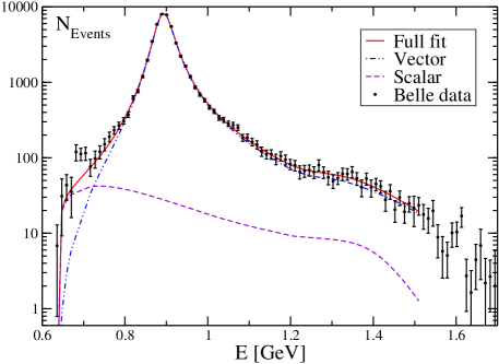
Figure 1: Fit result for the spectrum of $\tau\rightarrow K\pi\nu_{\tau}$. The data in black are from Belle Collaboration [2]. The dashed violet line represents the scalar form factor contribution fixed from the $K_{\mu 3}$ results, see text. The dot-dashed blue line is the vector form factor contribution and the solid red line gives the full result.

The introduction of the dispersive parametrizations Eqs. (9,3.2) which are valid in the full energy range allows to combine the $\tau\rightarrow K\pi\nu_{\tau}$ decay analysis with the $K_{\ell 3}$ one to further constrain the K$\pi$ form factors. Note that for the moment we cannot take into account the results on the vector form factor parameters coming from $K_{\mu 3}$ decays because we do not have the correlations between ln$C$ and $\lambda_{+}^{\prime}$ and $\lambda_{+}^{\prime\prime}$. In the future, a combined fit of the $\tau$ and $K_{\ell 3}$ decays should be performed using the same dispersive parametrization in order to take into account all the available data and the correlations between the two form factors.

4.2 Discussion

Since our fits are still preliminary we refrain from quoting final results. Instead, we concentrate in a discussion of the prospects of our analysis [23]. To do so, we show in Fig. 1 the contribution of the scalar form factor to the $\tau\rightarrow K\pi\nu_{\tau}$ decay spectrum, Eq. (18), where the value for ln$C$ has been taken from the $K_{\mu 3}$ analyses [1], $\mathrm{ln}C=0.2004\pm 0.0091$, and $\lambda_{0}^{\prime}$ has been determined from the sum-rule Eq. (17), $\lambda_{0}^{\prime}=13.71\cdot 10^{-3}$. The vector form factor has been fitted to the data with the two scalar form factor parameters fixed to the later values. Its contribution is also shown in Fig. 1 together with the total contribution to the decay spectrum. As can be seen, some information on $\bar{f}_{0}(s)$ can be obtained from $\tau\rightarrow K\pi\nu_{\tau}$ close to threshold ($s_{K\pi}$). But at present the Belle data alone are not precise enough to really be able to give strong constraints on $\bar{f}_{0}(s)$. A measurement of the forward-backward asymmetry would be very useful to di-sentangle the scalar and vector form factors [25]. As it has been already shown in Refs. [2, 3, 4, 5, 6], the $\tau\rightarrow K\pi\nu_{\tau}$ decay spectrum measurement gives interesting constraints on $\bar{f}_{+}(s)$ and in particular on the mass and width of $K^{*}(892)$. Note that in the Belle data, Fig. 1, there is a bump close to threshold given by three points, bins 6, 7 and 8 which cannot be accommodated by the form factor parametrizations and which does not seem to be present in the BaBar data [3]. Awaiting the more precise measurements of the $\tau\rightarrow K\pi\nu_{\tau}$ decays that are underway, an interesting possibility offered by the dispersive parametrization is to combine the $\tau$ decay analyses with the $K_{\ell 3}$ decays [7] and test the consistency of the determinations of the form factor parameters. As shown in Ref. [7], it allows for a very precise determination of $\lambda_{+}^{\prime}$ and $\lambda_{+}^{\prime\prime}$ since the correlations of these two parameters are of opposite sign in the two analyses. As for $\bar{f}_{0}(s)$, the combination allows for determining in addition to ln$C$, $\lambda_{0}^{\prime}$ directly from the data. Last but not least, this analysis offers a direct extraction of $|V_{us}|$ from $\tau\rightarrow K\pi\nu_{\tau}$ decays and an interesting consistency-test of the determination of $|V_{us}|$ from $\tau$ decays by comparing its value to the one coming from inclusive hadronic $\tau$ decays.

5 CONCLUSION

With the new measurements of $\tau\rightarrow K\pi\nu_{\tau}$ at the B factories [2, 3] and the forthcoming ones [26], a precise extraction of the K$\pi$ form factors becomes possible. To this end, we have built a physically well-motivated dispersive representation for the form factors. One interesting feature of this parametrization is that it allows to combine the $K_{\ell 3}$ and $\tau\rightarrow K\pi\nu_{\tau}$ analyses in order to increase the precision in the determination of the form factor parameters. This allows for stringent tests of the Standard Model and in particular for an extraction of $|V_{us}|$ directly from $\tau\rightarrow K\pi\nu_{\tau}$ decays.

References

- [1] M. Antonelli et al., Eur. Phys. J. C69 (2010) 399-424.
- [2] D. Epifanov et al. [Belle Collaboration], Phys. Lett. B 654 (2007) 65.
- [3] S. Paramesvaran [BaBar Collaboration], proceedings of Meeting of DPF 2009, arXiv:0910.2884 [hep-ex].
- [4] M. Jamin, A. Pich and J. Portoles, Phys. Lett. B 640 (2006) 176; ibid, Phys. Lett. B 664 (2008) 78.
- [5] B. Moussallam, Eur. Phys. J. C 53 (2008) 401.
- [6] D. R. Boito, R. Escribano and M. Jamin, Eur. Phys. J. C 59 (2009) 821.
- [7] D. R. Boito, R. Escribano and M. Jamin, JHEP 1009 (2010) 031.
- [8] V. Bernard, M. Oertel, E. Passemar and J. Stern, Phys. Lett. B 638 (2006) 480.
- [9] V. Bernard, M. Oertel, E. Passemar and J. Stern, Phys. Rev. D 80 (2009) 034034.
- [10] A. Kastner and H. Neufeld, Eur. Phys. J. C 57 (2008) 541.
- [11] V. Cirigliano, M. Giannotti and H. Neufeld, JHEP 0811 (2008) 006.
- [12] J. Erler, Rev. Mex. Fis. 50 (2004) 200.
- [13] F. V. Flores-Baez, Nucl. Phys. Proc. Suppl. 207-208 (2010) 141 and private communication.
- [14] H. Leutwyler and M. Roos, Z. Phys. C 25 (1984) 91; J. Bijnens and P. Talavera, Nucl. Phys. B 669 (2003) 341; M. Jamin, J. A. Oller and A. Pich, JHEP 0402 (2004) 047; V. Cirigliano et al., JHEP 0504 (2005) 006; V. Bernard and E. Passemar, Phys. Lett. B 661 (2008) 95.
- [15] See e.g. G. Colangelo et al., arXiv:1011.4408 [hep-lat] and references therein.
- [16] C. G. Callan and S. B. Treiman, Phys. Rev. Lett. 16 (1966) 153; R. F. Dashen and M. Weinstein, Phys. Rev. Lett. 22 (1969) 1337.
- [17] J. Gasser and H. Leutwyler, Nucl. Phys. B 250 (1985) 517; J. Bijnens and K. Ghorbani, arXiv:0711.0148 [hep-ph].
- [18] M. Antonelli et al. [FlaviaNet Working Group on Kaon Decays], arXiv:0801.1817 [hep-ph].
- [19] E. Passemar, PoS KAON09 (2009) 024.
- [20] K. M. Watson, Phys. Rev. 88, 1163 (1952).
- [21] G. P. Lepage and S. J. Brodsky, Phys. Lett. B 87 (1979) 359.
- [22] K. Nakamura et al. (Particle Data Group), J. Phys. G 37, 075021 (2010).
- [23] V. Bernard, D. R. Boito, E. Passemar, in preparation.
- [24] P. Buettiker, S. Descotes-Genon and B. Moussallam, Eur. Phys. J. C 33 (2004) 409.
- [25] L. Beldjoudi and T. N. Truong, Phys. Lett. B 351 (1995) 357.
- [26] D. M. Asner et al., Int. J. of Mod. Phys. A 24 Supplement 1 (2009).