When is social computation better than the sum of its parts?

Abstract

Social computation, whether in the form of searches performed by swarms of agents or collective predictions of markets, often supplies remarkably good solutions to complex problems. In many examples, individuals trying to solve a problem locally can aggregate their information and work together to arrive at a superior global solution. This suggests that there may be general principles of information aggregation and coordination that can transcend particular applications. Here we show that the general structure of this problem can be cast in terms of information theory and derive mathematical conditions that lead to optimal multi-agent searches. Specifically, we illustrate the problem in terms of local search algorithms for autonomous agents looking for the spatial location of a stochastic source. We explore the types of search problems, defined in terms of the statistical properties of the source and the nature of measurements at each agent, for which coordination among multiple searchers yields an advantage beyond that gained by having the same number of independent searchers. We show that effective coordination corresponds to synergy and that ineffective coordination corresponds to independence as defined using information theory. We classify explicit types of sources in terms of their potential for synergy. We show that sources that emit uncorrelated signals provide no opportunity for synergetic coordination while sources that emit signals that are correlated in some way, do allow for strong synergy between searchers. These general considerations are crucial for designing optimal algorithms for particular search problems in real world settings.

I Introduction

The ability of agents to share information and to coordinate actions and decisions can provide significant practical advantages in real-world searches. Whether the target is a person trapped by an avalanche or a hidden cache of nuclear material, being able to deploy multiple autonomous searchers can be more advantageous and safer than sending human operators. For example, small autonomous, possibly expendable robots could be utilized in harsh winter climates or on the battlefield.

In some problems, e.g. locating a cellular telephone via the signal strength at several towers, there is often a simple geometrical search strategy, such as triangulation, which works effectively. However, in search problems where the signal is stochastic or no geometrical solution is known, e.g. searching for a weak scent source in a turbulent medium, new methods need to be developed. This is especially true when designing autonomous and self-repairing algorithms for robotic agents Bourgault_2003 . Information theoretical methods provide a promising approach to develop objective functions and search algorithms to fill this gap. In a recent paper, Vergassola et al. demonstrated that infotaxis, which is motion based on expected information gain, can be a more effective search strategy when the source signal is weak than conventional methods such as moving along the gradient of a chemical concentration Vergassola_2007 . The infotaxis algorithm combines the two competing goals of exploration of possible search moves and exploitation of received signals to guide the searcher in the direction with the highest probability of finding the source Sulton_1998 .

To improve the efficiency of search by using more than one searcher requires determining under what circumstances a collective (parallel) search is better (faster) than the independent combination of the individual searches. Much heuristic work, anecdotally inspired by strategies in social insects and flocking birds couzin-2005-effective ; bonabeau-2000-swarm , has suggested that collective action should be advantageous in searches in real world complex problems, such as foraging, spatial mapping, and navigation. However, all approaches to date rely on simple heuristics that fail to make explicit the general informational advantages of such strategies.

The simplest extension of infotaxis to collective searches is to have multiple independent (uncoordinated) searchers that share information; this corresponds in general to a linear increase in performance with the number of searchers. However, given some general knowledge about the structure of the search, substantial increases in the search performance of a collective of agents can be achieved, often leading to exponential reduction in the search effort, in terms of time, energy or number of steps Seung_1992 ; Freund_1997 ; Fine_2002 . In this work we explore how the concept of information synergy can be leveraged to improve infotaxis of multiple coordinated searchers. Synergy corresponds to the general situation when measuring two or more variables together with respect to another (the target’s signal) results in a greater information gain than the sum of that from each variable separately Bettencourt_2007 ; Bettencourt_2008 . We identify the types of spatial search problems for which coordination among multiple searchers is effective (synergetic), as well as when it is ineffective, and corresponds to independence. We find that classes of statistical sources, such as those that emit uncorrelated signals (e.g. Poisson processes) provide no opportunity for synergetic coordination. On the other hand, sources that emit particles with spatial, temporal, or categorical correlations, do allow for strong synergy between searchers that can be exploited via coordinated motion. These considerations divide collective search problems into different general classes and are crucial for designing effective algorithms for particular applications.

II Information theory approach to stochastic search

Effective and robust search methods for the location of stochastic sources must balance the competing strategies of exploration and exploitation Sulton_1998 . On the one hand, searchers must exploit measured cues to guide their optimal next move. On the other hand, because this information is statistical, more measurements need to typically be made that are guided by different search scenarios. Information theory approaches to search achieve this balance by utilizing movement strategies that increase the expected information gain, which in turn is a functional of the many possible source locations. In this section we define the necessary formalism and use it to set up the general structure of the stochastic search problem.

II.1 Synergy and Redundancy

First we define the concepts of information, synergy and redundancy explicitly. Consider the stochastic variables $X_{i},i=1\ldots n$. Each variable $X_{i}$ can take on specific states, denoted by the corresponding lowercase letter, that is $X$ can take on a set of states $\{x\}$. For a single variable $X$ the Shannon entropy (henceforth “entropy”) is $S(X)=-\sum_{x}P(x)\log_{2}P(x)$, where $P(x)$ is the probability that the variable $X$ take on the value $x$ Cover_1991 . The entropy is a measure of uncertainty about the state of $X$, therefore entropy can only decrease or remain unchanged as more variables are measured. The conditional entropy of a variable $X_{1}$ given a second variable $X_{2}$ is $S(X_{1}|X_{2})=-\sum_{x_{1},x_{2}}P(x_{1},x_{2})\log_{2}(P(x_{1},x_{2})/P(x_{2}))\leq S(X_{1})$. The mutual information between two variables, which plays an important role in search strategy, is defined as the change in entropy when a variable is measured $I(X_{1},X_{2})=S(X_{1})-S(X_{1}|X_{2})\geq 0$. These definitions can be directly extended to multiple variables. For 3 variables, we make the following definition Schneidman_2003 : $R(X_{1},X_{2},X_{3})\equiv I(X_{1},X_{2})-I(\{X_{1},X_{2}\}|X_{3})$. This quantity measures the degree of “overlap” in the information contained in variables $X_{1}$ and $X_{2}$ with respect to $X_{3}$. If $R(X_{1},X_{2},X_{3})>0$, there is overlap and $X_{1}$ and $X_{2}$ are said to be redundant with respect to $X_{3}$. If $R(X_{1},X_{2},X_{3})<0$, more information is available when these variables are considered together than when considered separately. In this case $X_{1}$ and $X_{2}$ are said to be synergetic with respect to $X_{3}$. If $R(X_{1},X_{2},X_{3})=0$, $X_{1}$ and $X_{2}$ are independent Bettencourt_2007 ; Bettencourt_2008 .

II.2 Two-dimensional spatial search

We now formulate the two-dimensional stochastic search problem. We consider, for simplicity, the case of two searchers seeking to find a stochastic source located in a finite two-dimensional plane. This is a generalization of the single searcher formalism presented in Ref. Vergassola_2007 . At any time step, the searchers have positions $\{r_{i}\},i=1,2$ and observe some number of particles $\{h_{i}\}$ from the source. The searchers do not get information about the trajectories or speed of the particles; they only get information if a particle was observed or not. Therefore simple geometrical methods such as triangulation are not possible. Let the variable $R_{0}$ correspond to all the possible locations of the source $r_{0}$. The searchers compute and share a probability distribution $P^{(t)}(r_{0})$ for the source at each time index $t$. Initially the probability for the source is assumed to be to be uniform. After each measurement $\{h_{i},r_{i}\}$, the searchers update their estimated probability distribution of source positions via Bayesian inference. First the conditional probability $P^{(t+1)}(r_{0}|\{h_{i},r_{i}\})\equiv P^{(t)}(r_{0})P(\{h_{i},r_{i}\}|r_{0})/A$, is calculated, where $A$ is a normalization over all possible source locations as required by Bayesian inference. This is then assimilated via Bayesian update so that $P^{(t+1)}(r_{0})\equiv P^{(t+1)}(r_{0}|\{h_{i},r_{i}\})$.

If the searchers do not find the source at their present locations they choose the next local move using an infotaxis step to maximize the expected information gain. To describe the infotaxis step we first need some definitions. The entropy of the distribution $P^{(t)}(r_{0})$ at time $t$ is defined as $S^{(t)}(R_{0})\equiv-\sum_{r_{0}}P^{(t)}(r_{0})\log_{2}P^{(t)}(r_{0})$. In terms of a specific measurement $\{h_{i},r_{i}\}$ the entropy is (before the Bayesian update) $S^{(t)}_{\{h_{i},r_{i}\}}(R_{0})\equiv-\sum_{r_{0}}P^{(t)}(r_{0}|\{h_{i},r_{i}\})\log_{2}P^{(t)}(r_{0}|\{h_{i},r_{i}\})$. We define the difference between the entropy at time $t$ and the entropy at time $t+1$ after a measurement $\{h_{i},r_{i}\}$ to be $\Delta S^{(t+1)}_{\{h_{i},r_{i}\}}\equiv S^{(t+1)}_{\{h_{i},r_{i}\}}(R_{0})-S^{(t)}(R_{0})$.

Initially the entropy is at its maximum for a uniform prior: $S^{(0)}(R_{0})=\log_{2}N_{s}$, where $N_{s}$ is the number of possible locations for the source in a discrete space. For each possible joint move $\{r_{i}\}$, the change in expected entropy $\overline{\Delta S}$ is computed and the move with the minimum (most negative) $\overline{\Delta S}$ is executed. The expected entropy is computed by considering the reduction in entropy for all of the possible joint moves

$$\overline{\Delta S} =-\biggl{[}\sum_{i}P^{(t)}(R_{0}=r_{i})\biggr{]}S^{(t)}(R_{0})$$

$$+\biggl{[}1-\sum_{i}P^{(t)}(R_{0}=r_{i})\biggr{]}\Delta S^{(t+1)}_{\{h_{i},r_{i}\}}$$

$$\times\sum_{h_{1},h_{2}}\biggl{[}\sum_{r_{0}}P^{(t)}(r_{0})P^{(t+1)}(\{h_{i},r_{i}\}|r_{0})\biggr{]}.$$ (1)

The first term in Eq. (1) corresponds to one of the searchers finding the source in the next time step (the final entropy will be $S=0$ so $\overline{\Delta S}=-S$). The second term considers the reduction in entropy for all possible measurements at the proposed location, weighted by the probability of each of those measurements. The probability of the searchers obtaining the measurement $\{h_{i}\}$ at the location $\{r_{i}\}$ is given by the trace of the probability $P^{(t+1)}(\{h_{i},r_{i}\}|r_{0})$ over all possible source locations.

III Correlated stochastic source and synergy of searchers

The expected entropy reduction $\overline{\Delta S}$ is calculated for joint moves of the searchers, that is, all possible combinations of individual moves. Compared with multiple independent searchers this calculation incurs some extra computational cost. Thus, when designing a search algorithm, it is important to know whether an advantage (synergy) can be gained by considering joint moves instead of individual moves. Since the search is based on optimizing the maximum information gain we need to explore if joint moves are synergetic or redundant. In this section we will show how correlations in the source affect the synergy and redundancy of the search.

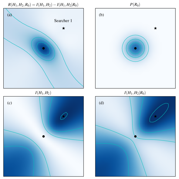
Figure 1: Synergy for the two searcher problem with angular correlations. (a) $R(H_{1},H_{2},R_{0})$ as a function of the position of searcher 2 ($r_{2}$) for a fixed location of searcher 1 ($r_{1}$, shown as a black star). The most probable source location is in the center (black dot). The white to blue scale indicates $R=0$ to $R=-2\times 10^{-5}$ and we note that $R\leq 0$ everywhere. The darker color indicates stronger synergy values when searcher 2 is near the source. The synergy is less when searcher 2 is away from or on the opposite side ($R\approx 0$) of the source. (b) The probability distribution of source locations, peaked at the center: $P(\vec{r_{0}})=A\exp{(-|\vec{r_{0}}|^{2}/0.02)}$, where $A=1/\sum_{\vec{r_{0}}}P(\vec{r_{0}})$ is a normalization factor. White to blue indicates $P=0$ to $P=0.02$. (c) $I(H_{1},H_{2})$; (d) $I(H_{1},H_{2}|R_{0})$. In (c) and (d) white to blue indicates $I=0$ to $I=6\times 10^{-5}$. Contour lines have been added to guide the eye. In all frames the data is plotted in a two-dimensional spatial domain of $x,y=[-0.5,0.5]$ and all vectors are measured from the origin $x=0,y=0$. The parameter $\sigma^{2}=1.1$ in Eq. 5.

In the following we will assume there are no radial correlations between particles emitted from the source and that the probability of detecting particles decays with distance to the source. For each particle emitted from the source, the searcher $i$ has an associated actual probability $\pi_{i}(r_{0})$ of catching the particle. The probability $\pi_{i}(r_{0})$ is defined in terms of a possible source location $r_{0}$ and the location $r_{i}$ of searcher $i$: $\pi_{i}(r_{0})=B\exp{(-|\vec{r}_{i}-\vec{r_{0}}|^{2})}$, where $\{r_{i}\}$ is the set of all the searcher positions and $B$ is a normalization constant. Note that this is just the radial component of the probability; if there are angular correlations these are treated separately. We may now write $R$, as a function of the variables $R_{0}$, $H_{1}$, and $H_{2}$, in terms of the conditional probabilities:

$$R(H_{1},H_{2},R_{0})=$$

$$\sum_{h_{1},h_{2},r_{0}}P(r_{0},h_{1},h_{2})\log_{2}\frac{P(h_{1}|r_{0})P(h_{2}|r_{0})P(h_{2}|h_{1})}{P(h_{2})P(h_{1},h_{2}|r_{0})}.$$ (2)

It is sufficient for $R\neq 0$ that the argument of the logarithm differs from $1$. This can be achieved even if measurements are conditionally independent (redundancy), mutually independent (synergy), or when neither of these conditions apply.

III.1 Uncorrelated signals: Poisson source

First, consider a source which emits particles according to a Poisson process with known mean $\lambda_{0}$ so emitted particles are completely uncorrelated spatially and temporally. If searcher 1 is able to get a particle that has already been detected by searcher 2, it is clear that the searchers are completely independent and there is no chance of synergy. It may appear at first that implementing a simple exclusion where two searchers cannot get the same particle would be enough to foster cooperation between searchers. We will instead show that it is the Poisson nature of the source that makes synergy impossible, even under mutual exclusion of the measurements.

The probability of the measurement $\{h_{i}\}$ is given by

$$P(\{h_{i},r_{i}\}|r_{0})=\sum_{h_{s}=\sum_{i}h_{i}}^{\infty}P_{0}(h_{s},\lambda_{0})M(\{\pi_{i}(r_{0})\},\{h_{i}\},h_{s}).$$ (3)

The sum is over all possible values of $h_{s}$, weighted by the Poisson probability mass function with the known mean $\lambda_{0}$. $M$ is the probability mass function of the multinomial distribution for that measurement; it handles the combinatorial degeneracy and the exclusion. It is not difficult to show by summing over $h_{s}$ that $P(\{h_{i},r_{i}\}|r_{0})$ can be written as a product of Poisson distributions with effective means $\lambda_{0}\pi_{i}$,

$$P(\{h_{i},r_{i}\}|r_{0})=\frac{\lambda_{0}^{\sum_{i}h_{i}}e^{-\lambda_{0}\sum_{i}\pi_{i}}\prod_{i}\pi_{i}^{h_{i}}}{\prod_{i}(h_{i}!)}=\prod_{i}P_{0}(h_{i},\lambda_{0}\pi_{i}).$$ (4)

At this point we consider whether a search like this can be synergetic for the 2 searcher case. Eq. (4) shows that the two measurements are conditionally independent and therefore $P(h_{1},h_{2}|r_{0})=P(h_{1}|r_{0})P(h_{2}|r_{0})$. It follows from Eq. (2) that $R(H_{1},H_{2},R_{0})$ $=I(H_{1},H_{2})\geq 0$. Therefore the searchers are either redundant (if the measurements interfere with each other) or independent with respect to the source. Synergy is impossible so that searchers gain no advantage by considering joint moves. The only advantage of coordination comes possibly from avoiding positions that lead to a decrease in performance of the collective due to competition for the same signal.

III.2 Correlated signals: angular biases

We now consider a source that emits particles that are spatially correlated. We assume for simplicity that at each time step the source emits 2 particles. The first particle is emitted at a random angle $\theta_{h_{1}}$ chosen uniformly from $[0,2\pi)$. The second particle is emitted at an angle $\theta_{h_{2}}$ with probability

$$P(\theta_{h_{2}}|\theta_{h_{1}})=D\exp{[-(|\theta_{h_{1}}-\theta_{h_{2}}|-\pi)^{2}/\sigma^{2}]}\equiv f,$$ (5)

where $D$ is a normalization factor. The searchers are assumed to know the variance $\sigma$ for simplicity; this is a reasonable assumption if the searchers have any information about the nature of the target (just as for the Poisson source they had statistical knowledge of the parameter $\lambda_{0}$). The calculation of the conditional probability $P(\{h_{i},r_{i}\}|r_{0})$ requires some care. Specifically, this quantity is the probability of the measurement $\{h_{i}\}$, assuming a certain source position. Since there are 2 particles emitted at each time step, there are 4 possible cases, each with a different probability, as shown in Table 1. Here $\theta_{h_{1}}$ and $\theta_{h_{2}}$ are calculated from $r_{1}$ and $r_{2}$, respectively: $\theta_{h_{i}}\equiv\arctan{\frac{r_{0,y}-r_{i,y}}{r_{0,x}-r_{i,x}}}$. Note that the $\pi_{i}$ are functions of $r_{0}$. The coefficient $D$ is chosen such that $\tfrac{1}{N}\sum_{h_{2}}\sum_{r_{2}}P(\{h_{1},h_{2},r_{1},r_{2}\}|r_{0})=P(\{h_{1},r_{1}\}|r_{0})$, corresponding to the normalization condition $\tfrac{1}{N}\sum_{r_{2}}f=1$.

$\{h_{1},h_{2}\}$	$\{1,1\}$	$\{1,0\}$	$\{0,1\}$	$\{0,0\}$
$P(\{h_{1},r_{1}\}|r_{0})$	$\pi_{1}$	$\pi_{1}$	$1-\pi_{1}$	$1-\pi_{1}$
$P(\{h_{2},r_{2}\}|r_{0})$	$\pi_{2}$	$\pi_{2}$	$1-\pi_{2}$	$1-\pi_{2}$
$P(\{h_{1},h_{2},r_{1},r_{2}\}|r_{0})$	$\pi_{1}\pi_{2}f^{2}$	$\pi_{1}f\bigl{(}1-\pi_{2}f\bigr{)}$	$\pi_{2}f\bigl{(}1-\pi_{1}f\bigr{)}$	$(1-\pi_{1}f)(1-\pi_{2}f)$

Table 1: Probability calculation for all possible states in the correlated source search. Here $\pi_{i}(r_{0})=B\exp{(-|\vec{r}_{i}-\vec{r_{0}}|^{2})}$ is written as $\pi_{i}$ to save space.

Figure 1 shows the value of $R(H_{1},H_{2},R_{0})$ and the values of the mutual informations $I(H_{1},H_{2})$ and $I(H_{1},H_{2}|R_{0})$ for each possible position $r_{2}$ of searcher 2. We assume a nonuniform, peaked probability distribution for the source [Figure 1(b)] and that the position of searcher 1 is fixed. In this setup we see that $R<=0$ for every possible position of searcher 2 indicating that only synergy is possible. This is a consequence of the angular spatial correlation between the particles emitted by the source. The synergy is highest near the source location, where the source probability is strongly peaked, and falls off rapidly away from the source location. Furthermore there is little to no synergy near searcher 1 since in that region it is very unlikely that both searchers would simultaneously observe a particle. The area of greatest synergy corresponds to the most probable source locations for both searchers to simultaneously observe a particle. $P(r_{0})$ is very flat at the boundaries; thus $R_{0}$ contributes little to $I(H_{1},H_{2}|R_{0})$ in the lower left corner and $R$ is small.

IV Conclusion

In the real world, communication between agents, as well as centralized or decentralized real-time computation can be difficult or expensive. Therefore it is important to consider the classes of search problems for which coordination between searchers can achieve quantitative advantages over independent agents. In this work we studied search algorithms for autonomous agents looking for the spatial location of a stochastic source. We defined the search problem for multiple agents in terms of infotaxis [see Eq. (1)]. We also showed why synergy gives rise to an advantage in this type of search. We considered two types of sources. We first demonstrated that a source emitting uncorrelated particles will afford no opportunity for synergy (see Section III.1). In a search for a Poisson source, multiple coordinated searchers (ones that consider sets of joint moves rather than each considering an independent move) can not hope to do better than multiple independent searchers. Next we showed that, for a source emitting particles with (angular) correlations (see Section III.2), only synergy or independence is possible (see Fig. 1). The ability of the searchers to leverage synergy depends strongly on their ability to estimate with some accuracy the probability distribution of source locations. These general considerations are crucial for the exploitation of social computation in terms of the design of optimal collective algorithms in particular applications. The next step to making this approach applicable to a broader class of problems, including those not limited to spatial searches, is to generalize the results to more than 2 searchers and to explore how synergy may be best leveraged to give increases in search speed and efficiency.

This paper is released under LA-UR 09-00432.

References

- (1) F. Bourgault, T. Furukawa, and H.F. Durrant-Whyte. Coordinated decentralized search for a lost target in a Bayesian world. Intelligent Robots and Systems, 2003. (IROS 2003). Proceedings. 2003 IEEE/RSJ International Conference on, 1:48, Oct. 2003.
- (2) M. Vergassola, E. Villermaux, and B. I. Shraiman. “Infotaxis” as a strategy for searching without gradients. Nature, 445:406, 2007.
- (3) R. S. Sulton and A. G. Barto. Reinforcement learning: an introduction. MIT Press, Cambrigde MA, 1998.
- (4) Iain D. Couzin, Jens Krause, Nigel R. Franks, and Simon A. Levin. Effective leadership and decision-making in animal groups on the move. Nature, 433:513, 2005.
- (5) E. Bonabeau and G. Theraulaz. Swarm smarts. Scientific American, pages 72–79, Mar. 2000.
- (6) H. S. Seung, M. Opper, and H. Sompolinsky. Query by committee. In COLT ’92: Proceedings of the fifth annual workshop on Computational learning theory, page 287, 1992.
- (7) Y. Freund, E. Shamir, and N. Tishby. Selective sampling using the query by committee algorithm. In Machine Learning, page 133, 1997.
- (8) S. Fine, R. Gilad-Bachrach, and E. Shamir. Query by committee, linear separation and random walks. Theor. Comput. Sci., 284(1):25, 2002.
- (9) Luis M. A. Bettencourt, Greg J. Stephens, Michael I. Ham, and Guenter W. Gross. Functional structure of cortical neuronal networks grown in vitro. Phys. Rev. E, 75:021915, 2007.
- (10) L. M. A. Bettencourt, V. Gintautas, and M. I. Ham. Identification of functional information subgraphs in complex networks. Phys. Rev. Lett., 100:238701, 2008.
- (11) T. M. Cover and J. A. Thomas. Elements of Information Theory. Wiley, New York, 1991.
- (12) E. Schneidman, W. Bialek, and M. J. Berry II. Synergy, redundancy, and independence in population codes. J. Neurosci., 23:11539, 2003.