3D+1 Lorentz type soliton in air

Abstract

Up to now the long range filaments have been considered as a balance between Kerr focusing and defocusing by plasma generation in the nonlinear focus. However, it is difficult to apply the above explanation of filamentation in far-field zone. There are basically two main characteristics which remain the same at these distances - the super broad spectrum and the width of the core, while the power in a stable filament drops to the critical value for self-focusing. At such power the plasma and higher-order Kerr terms are too small to prevent self-focusing. We suggest here a new mechanism for stable soliton pulse propagation in far-away zone, where the power of the laser pulse is slightly above the critical one, and the pulse comprises super-broad spectra. For such pulses the diffraction is not paraxial and an initially symmetric Gaussian pulse takes parabolic form at several diffraction lengths . The stable soliton propagation appears as a balance between the divergent parabolic type diffraction of broadband optical pulses and the convergent nonlinear refractive index due to the intensity profile. We investigate more precisely the nonlinear third order polarization, using into account the carrier-to envelope phase. This additional phase transforms the third harmonic term to THz or GHz one, depending on the spectral width of the pulse.

I Introduction

In the process of investigating the filamentation of a power femtosecond (fs) laser pulse many new physical effects have been observed, such as long-range self-channeling MOU ; WO ; MEC , coherent and incoherent radial and forward THz emission TZ ; DAMYZ ; DAHO , asymmetric pulse shaping, super-broad spectra HAU1 ; HAU2 ; COU1 ; SKUP ; CHIN1 ; KASP1 and others. The role of the different mechanisms in near zone (up to $1-2$ $m$ from the source) has been investigated experimentally and by numerical simulations, and most processes in this zone are well explained COU ; KAN ; FAC ; KOL1 . When a fs pulse with power of several $P_{cr}=\pi(0.61\lambda_{0})^{2}/(8n_{0}n_{2})$ starts from the laser source a slice-by-slice self-focussing process takes place SHEN . At a distance of one-two meters the pulse self-compresses, enlarging the $k_{z}$ spectrum to super-broad asymmetric spectrum $\triangle k_{z}\approx k_{0}$. The process increases the core intensity up to tens of $10^{13}W/cm^{2}$, where different types of plasma ionization, multi-photon processes and higher-order Kerr terms appear KASP2 . Usually, the basic model of propagation in near the zone is a scalar spatio-temporal paraxial equation including all the above mentioned mechanisms COU ; KAN ; KASP2 . The basic model is natural in the near zone because of the fact that the initial fs pulse contains a narrow-band spectrum $\triangle k_{z}<<k_{0}$. Thus, the paraxial spatio-temporal model gives a good explanation of nonlinear phenomena such as conical emission, X-waves, spectral broadening to the high frequency region and others. In far-away zone (propagation distance more than $2-3$ meters) plasma ionization and higher-order Kerr terms are admitted also as necessary for a balance between the self-focussing and plasma defocussing and for obtaining long range self-channeling in gases.

However, the above explanation of filamentation is difficult to apply in far-away zone. There are basically two main characteristics which remain the same at these distances - the superbroad spectrum and the width of the core, while the intensity in a stable filament drops to a value of $10^{12}W/cm^{2}$ COU ; KASP2 . The plasma and higher-order Kerr terms are too small to prevent self-focussing. The observation of long-range self-channeling MECH ; DUB ; BERN without ionization also leads to change the role of plasma in the laser filamentation.

In addition, there are difficulties with the physical interpretation of the THz radiation as a result of plasma generation. The plasma strings formed during filamentation should emit incoherent THz radiation in a direction orthogonal to the propagation axis. The nature of the THz emission, measured in DAHO is different. Instead of being emitted radially, it is confined to a very narrow cone in the forward direction. The contribution from ionization in far-away zone is negligible KASP2 and this is the reason to look for other physical mechanism which could cause THz or GHz radiations. Our analysis on the third order nonlinear polarization of pulses with broadband spectrum indicates that the nonlinear term in the corresponding envelope equation oscillates with frequency proportional to the group and phase velocity difference $\Omega_{nl}=3(k_{0}v_{ph}-v_{gr}\triangle k_{z})$. Actually, this is three times the well-known Carrier-to Envelope Phase (CEP) difference EXTR . This oscillation induces THz generation, where the generated frequency is exactly $\Omega_{THz}=93GHz$ for a pulse with superbroad spectrum $\triangle k_{z}\approx k_{0}$ with carryier wavelength $800$ $nm$.

Physically, one dimensional Schrödinger solitons in fibers appear as a balance between the Kerr nonlinearity and the negative dispersion HAS ; AGR ; SER1 . On the other hand, if we try to find 2D+1 and spatio-temporal solitons in Kerr media, the numerical and the real experiments demonstrate that there is no balance between the plane wave paraxial diffraction - dispersion and the Kerr nonlinearity. This leads to instability and self-focusing of a laser beam or initially narrow band optical pulse. Recently Serkin in SER2 suggested stable soliton propagation and reducing the 3D soliton problem to one dimensional, with introducing trapping potential in Bose - Einstein condensates.

In this paper we present a new mathematical model, on the basis of the Amplitude Envelope (AE) equation, up to second order of dispersion, without using paraxial approximation. In the non-paraxial zone the diffraction of pulses with superbroad spectrum or pulses with a few cycles under the envelope is closer to wave type KOV1 . For such pulses, a new physical mechanism of balance between nonparaxial (wave-type diffraction) and third order nonlinearity appears. Exact analytical three-dimensional bright solitons in this regime are found.

II Linear regime of narrow band and broad band optical pulses

The paraxial spatio-temporal envelope equation governs well the transverse diffraction and the dispersion of fs pulses up to $6-7$ cycles under the envelope. This equation relies on one approximation obtained after neglecting the second derivative in the propagation direction and the second derivative in time from the wave equation CHRIS or from the $3D+1$ AE equation BRAB . In air, the series of $k^{2}(\omega)$ are strongly convergent up to one cycle under the envelope and this is the reason why the AE equation is correct up to the single-cycle regime.

The linearized AE, governing the propagation of laser pulses when the dispersion is limited to second order, is:

$$-2ik_{0}\left(\frac{\partial A}{\partial z}+\frac{1}{v_{gr}}\frac{\partial A}{\partial t}\right)=\Delta A-\frac{1+\beta}{v_{gr}^{2}}\frac{\partial^{2}A}{\partial t^{2}},$$ (1)

where $\beta=k"k_{0}v_{gr}^{2}$ is a number representing the influence of the second order dispersion. In vacuum and dispesionless media the following Diffraction Equation (DE) ($v\sim c$ ) is obtained:

$$-2ik_{0}\left(\frac{\partial V}{\partial z}+\frac{1}{v}\frac{\partial V}{\partial t}\right)=\Delta V-\frac{1}{v^{2}}\frac{\partial^{2}V}{\partial t^{2}}.$$ (2)

We solve AE (1) and DE (2) by applying spatial Fourier transformation to the amplitude functions $A$ and $V$. The fundamental solutions of the Fourier images $\hat{A}$ and $\hat{V}$ in ($k_{x},k_{y},\triangle k_{z},t$) space are:

$$\hat{A}=\hat{A}(k_{x},k_{y},\triangle k_{z},t=0)\times$$

$$\exp\left\{i\frac{v_{gr}}{\beta+1}\left(k_{0}\pm\sqrt{k_{0}^{2}+(\beta+1)\left({k_{x}}^{2}+{k_{y}}^{2}+{\triangle k_{z}}^{2}-2k_{0}\triangle k_{z}\right)}\right)t\right\},$$ (3)

$$\hat{V}=\hat{V}(k_{x},k_{y},\triangle k_{z},t=0)\exp\left\{iv\left(k_{0}\pm\sqrt{{k_{x}}^{2}+{k_{y}}^{2}+({\triangle k_{z}}-k_{0})^{2}}\right)t\right\},$$ (4)

respectively. In air $\beta\simeq 2.1\times 10^{-5}$, AE (1) is equal to DE (2), and the dispersion is negligible compared to the diffraction. We solve analytically the convolution problem (4) for initial Gaussian light bullet of the kind $V(x,y,z,t=0)=\exp\left(-(x^{2}+y^{2}+z^{2})/2r_{0}^{2}\right)$. The corresponding solution is:

$$V(x,y,z,t)=\frac{i}{2\hat{r}}\exp\left[-\frac{k_{0}^{2}r^{2}_{0}}{2}+ik_{0}(vt-z)\right]\times$$

$$\Biggr{\{}i(vt+\hat{r})\exp\left[-\frac{1}{2r^{2}_{0}}(vt+\hat{r})^{2}\right]erfc\left[\frac{i}{\sqrt{2}r_{0}}(vt+\hat{r})\right]$$ (5)

$$-i(vt-\hat{r})\exp\left[-\frac{1}{2r^{2}_{0}}(vt-\hat{r})^{2}\right]erfc\left[\frac{i}{\sqrt{2}r_{0}}(vt-\hat{r})\right]\Biggr{\}},$$

where $\hat{r}=\sqrt{x^{2}+y^{2}+(z-ir^{2}_{0}k_{0})^{2}}$. On the other hand, multiplying the solution (II) with the carrier phase, we obtain solution of the wave equation $E\left(x,y,z,t\right)=V\left(x,y,z,t\right)\exp{\left(i(k_{0}z-\omega_{0}t)\right)}$, where $\omega_{0}$ and $k_{0}$ are the carrier frequency and carrier wave number in the wave packet:

$$\Delta E=\frac{1}{v^{2}}\frac{\partial^{2}E}{\partial t^{2}},$$ (6)

$$E(x,y,z,t)=\frac{i}{2\hat{r}}\exp\left(-\frac{k_{0}^{2}r^{2}_{0}}{2}\right)\times$$

$$\Biggr{\{}i(vt+\hat{r})\exp\left[-\frac{1}{2r^{2}_{0}}(vt+\hat{r})^{2}\right]erfc\left[\frac{i}{\sqrt{2}r_{0}}(vt+\hat{r})\right]$$ (7)

$$-i(vt-\hat{r})\exp\left[-\frac{1}{2r^{2}_{0}}(vt-\hat{r})^{2}\right]erfc\left[\frac{i}{\sqrt{2}r_{0}}(vt-\hat{r})\right]\Biggr{\}}.$$

A systematic study on the different kinds of exact solutions and methods for solving wave equation (6) was performed recently in KIS . Here, as in KOV1 we suggest another method: Starting with the ansatz $E\left(x,y,z,t\right)=V\left(x,y,z,t\right)\exp{\left(i(k_{0}z-\omega_{0}t)\right)}$, we separate the main phase and reduce the wave equation to $3D+1$ parabolic type one (2). Thus, the initial value problem can be solved and exact (II) (or numerical) solutions of the corresponding amplitude equation (2) can be obtained. The solution (II), multiplied by the main phase, gives an exact solution (II) of the wave equation (6). To investigate the evolution of optical pulses at long distances, it is convenient to rewrite AE (1) equation in Galilean coordinate system $t^{\prime}=t;z^{\prime}=z-v_{gr}t$:

$$-i\frac{2k_{0}}{v_{gr}}\frac{\partial A}{\partial t^{\prime}}=\Delta_{\bot}A-\beta\frac{\partial^{2}A}{\partial z^{\prime 2}}-\frac{1+\beta}{v_{gr}^{2}}\left(\frac{\partial^{2}A}{\partial t^{\prime 2}}-2v_{gr}\frac{\partial^{2}A}{\partial t^{\prime}\partial z^{\prime}}\right).$$ (8)

Pulses governed by DE (2) move with phase velocity and the transformation is $t^{\prime}=t;z^{\prime}=z-vt$:

$$-i\frac{2k_{0}}{v}\frac{\partial V}{\partial t^{\prime}}=\Delta_{\bot}V-\frac{1}{v^{2}}\left(\frac{\partial^{2}V}{\partial t^{\prime 2}}-2v\frac{\partial^{2}V}{\partial t^{\prime}\partial z^{\prime}}\right).$$ (9)

Here, $\Delta_{\bot}=\frac{\partial^{2}}{\partial x^{2}}+\frac{\partial^{2}}{\partial y^{2}}$ denotes the transverse Laplace operator. The corresponding fundamental solution of AE equation (8) in Galilean coordinates is:

$$\hat{A}_{G}(k_{x},k_{y},\triangle k_{z},t)=\hat{A}_{G}(k_{x},k_{y},\triangle k_{z},t=0)\times$$

(10)

$$\exp\Biggr{\{}i\frac{v_{gr}}{\beta+1}\left[k_{0}-(\beta+1)\triangle k_{z}\pm\sqrt{\left(k_{0}-(\beta+1)\triangle k_{z}\right)^{2}+(\beta+1)(k_{x}^{2}+k_{y}^{2}-\beta\triangle k_{z}^{2})}\right]t\Biggr{\}},$$

while the fundamental solution of DE (9) becomes:

$$\hat{V}_{G}=\hat{V}_{G}(k_{x},k_{y},\triangle k_{z},t=0)\times$$

(11)

$$\exp\Biggr{\{}iv\left[k_{0}-\triangle k_{z}\pm\sqrt{\left(k_{0}-\triangle k_{z}\right)^{2}+k_{x}^{2}+k_{y}^{2}}\right]t\Biggr{\}}.$$

The analytical solution of (II) for initial pulse in the form of Gaussian bullet is the same as (II), but with new radial component $\hat{r}=\sqrt{x^{2}+y^{2}+(z+vt-ir^{2}_{0}k_{0})^{2}}$ translated in space and time. The numerical and analytical solutions of AE (1) and DE (2) are equal to the solutions of the equations AE (8) and DE (9) in Galilean coordinates with only one difference: in Laboratory frame the solutions translate in $z$-direction , while in Galilean frame the solutions stay in the centrum of the coordinate system.

The basic theoretical studies governed laser pulse propagation have been performed in so called ”local time” coordinates $z=z$; $\tau=t-z/v_{gr}$. In order to compare our investigation with these results, we need to rewrite AE equation (1) for the amplitude function $A$ in the same coordinate system. Thus Eq. (1) becomes:

$$-2ik_{0}\frac{\partial A}{\partial z}=\Delta_{\bot}A+\frac{\partial^{2}A}{\partial z^{2}}-\frac{2}{v_{gr}}\frac{\partial^{2}A}{\partial\tau\partial z}-\frac{\beta}{v_{gr}^{2}}\frac{\partial^{2}A}{\partial\tau^{2}}.$$ (12)

Since this is a parabolic type equation with low order derivative on $z$, we apply Fourier transform to the amplitude function in form: $\hat{A}\left(k_{x},k_{y},\triangle\omega,z\right)=FFF\left[A\left(x,y,z,t\right)\right]$, where $FFF$ denotes 3D Fourier transform in $x,y,\tau$ space and $\triangle\omega=\omega-\omega_{0}$; $\triangle k_{z}=\triangle\omega/v_{gr}$ are the spectral widths in frequency and wave vector domains correspondingly. The following ordinary differential equation in $\left(k_{x},k_{y},\triangle\omega,z\right)$ space is obtained:

$$-2i\left(k_{0}-\frac{\triangle\omega}{v_{gr}}\right)\frac{\partial\hat{A}}{\partial z}=-\left(k_{x}^{2}+k_{y}^{2}-\frac{\beta\triangle\omega^{2}}{v_{gr}^{2}}\right)\hat{A}+\frac{\partial^{2}\hat{A}}{\partial z^{2}}.$$ (13)

As can be seen from (13), if the second derivative on $z$ is neglected,then the paraxial spatio-temporal approximation is valid. Equation (13) is more general and we will estimate where we can apply spatio-temporal paraxial optics (PO), and where PO does not works. The fundamental solution of (13) is:

$$\hat{A}\left(k_{x},k_{y},\triangle\omega,z\right)=\hat{A}\left(k_{x},k_{y},\triangle\omega,0\right)\times$$

$$\exp\left\{i\left[\left(k_{0}-\frac{\triangle\omega}{v_{gr}}\right)\mp\sqrt{\left(k_{0}-\frac{\triangle\omega}{v_{gr}}\right)^{2}+k_{x}^{2}+k_{y}^{2}-\frac{\beta\triangle\omega^{2}}{v_{gr}^{2}}}\right]z\right\}.$$ (14)

The analysis of the fundamental solution (II) of the equation (13) is performed in two basic cases:

a: Narrow band pulses - from nanosecond up to $50-100$ femtosecond laser pulses, where the conditions:

$$\frac{\beta\triangle\omega^{2}}{v_{gr}^{2}}\leq k_{x}^{2}\sim k_{y}^{2}<<k_{0}^{2};\ \triangle k_{z}=\frac{\triangle\omega}{v_{gr}}<<k_{0}$$ (15)

are satisfied, and the wave vector’s difference $k_{0}-\triangle\omega/v_{gr}$ can be replaced by $k_{0}$. Using the low order of the Taylor expansion and the minus sign in front of the square root from the initial conditions, equation (II) is transformed in a spatio - temporal paraxial generalization of the kind:

$$\hat{A}\left(k_{x},k_{y},\triangle\omega,z\right)=\hat{A}\left(k_{x},k_{y},\triangle\omega,0\right)\exp\left[i\left(\frac{k_{x}^{2}+k_{y}^{2}-\frac{\beta\triangle\omega^{2}}{v_{gr}^{2}}}{2k_{0}}\right)z\right].$$ (16)

From (16) the evolution of the narrow band pulses becomes obvious: while the transverse projection of the pulses enlarges by the Fresnel’s law, the longitudinal temporal shape will be enlarged in the same away, proportionally to the dispersion parameter $\beta$. Such shaping of pulses with initially narrow band spectrum is demonstrated in Fig.1, where the typical Fresnel diffraction of the intensity profile (spot $(x,y)$ projection) is presented. The numerical experiment is performed for $100$ femtosecond Gaussian initial pulse at $\lambda=800$ nm, $\Delta k_{z}<<k_{0}$, $z_{0}=30\mu m$, $r_{0}(x,y)=60\mu m$, with $37.5$ cycles under envelope propagating in air ($\beta=2.1\times 10^{-5}$). The result is obtained by solving numerically the inverse Fourier transform of the fundamental solution (II) of the AE equation in the local time frame (12). The spot enlarges twice at one diffraction length $z_{diff}=r_{0}^{2}k_{0}$. Fig. 2 presents the intensity side $(x,\tau)$ projection of the same pulse. We should note that while the spot ($(x,y)$ projection) enlarges considerably due to the Fresnel law, the longitudinal time shape (the $\tau$ projection) remains the same on several diffraction lengths from the small dispersion in air. The diffraction - dispersion picture, presented by the side $(x,\tau)$ projection of the pulse, gives idea of what should happen in the nonlinear regime: the plane wave diffraction with a combination of parabolic type nonlinear Kerr focusing always leads to self-focusing for narrow-band ($\Delta k_{z}<<k_{0}$) pulses. The same Taylor expansion for narrow band pulses can be performed to fundamental solutions of the equation in Laboratory (II) and Galilean (II) frames.

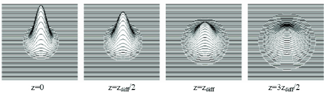
Figure 1: Plot of the waist (intensity’s) projection $|A(x,y)|^{2}$ of a $100$ $fs$ Gaussian pulse at $\lambda=800$ $nm$, with initial spot $r_{0}=60$ $\mu m$, and longitudinal spatial pulse duration $z_{0}=30$ $\mu m$, as solution of the linear equation in local time (12) on distances expressed by diffraction lengths. The spot deformation satisfies the Fresnel diffraction law and on one diffraction length $z=z_{diff}$ the diameter of the spot increases twice, while the maximum of the pulse decreases with the same factor.

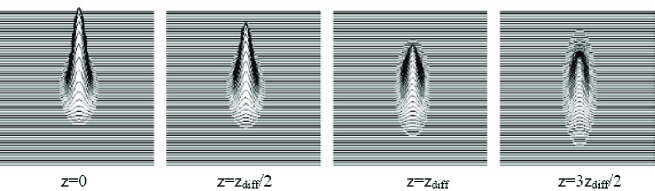
Figure 2: Side ($x,\tau$) projection of the intensity $|A(x,\tau)|^{2}$ for the same optical pulse as in Fig. 1. The ($x,y$) projection of the pulse diffracts considerably following the Fresnel law, while the ($\tau$) projection on several diffraction lengths preserves its initial shape due to the small dispersion. The diffraction - dispersion picture, presented by the side $(x,\tau)$ projection, gives idea of what should happen in the nonlinear regime: the plane wave diffraction with a combination of parabolic type nonlinear Kerr focusing always leads to self-focusing for narrow-band ($\triangle k_{z}<<k_{0}$) pulses.

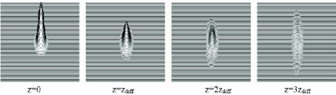
Figure 3: Side ($x,z$) projection of the intensity $|A(x,z^{\prime})|^{2}$ for a normalized $10$ fs Gaussian initial pulse at $\lambda=800$ nm, $\triangle k_{z}\simeq k_{0}/3$, $z_{0}=r_{0}/2$, and only $3$ cycles under the envelope (large-band pulse $\triangle k_{z}\approx k_{0}$), obtained numerically from the AE equation (8) in Galilean frame. At $3$ diffraction lengths a divergent parabolic type diffraction is observed. In nonlinear regime a possibility appear: the divergent parabolic type diffraction for large-band pulses to be compensated by the converged parabolic type nonlinear Kerr focusing.

b: broad band pulses - from attosecond up to $20-30$ femtosecond pulses, where the conditions:

$$\frac{\triangle\omega^{2}}{v_{gr}^{2}}\sim k_{0}^{2}\propto k_{x}^{2}\sim k_{y}^{2}$$ (17)

are satisfied. In this case we can not use Taylor expansion of the spectral kernels in Laboratory (II), Galilean (II) and local time (II) frames. The spectral kernels are in square root and we can expect evolution governed by wave diffraction. That why for broadband pulses we can expect curvature (parabolic deformation) of the intensity profile of the $(x,z)$ or $(x,\tau)$ side projection. Fig 3. present the evolution of the intensity (side $(x,z)$ projection) of a normalized $10$ fs Gaussian initial pulse at $\lambda=800$ nm; $\Delta k_{z}\simeq k_{0}/3$; $z_{0}=r_{0}/2$; and only $3$ cycles under the envelope (broadband pulse), obtained numerically from AE equation (8) in Galilean frame. The solution confirms the experimentally observed parabolic type diffraction for few cycle pulses. And here appears the main physical question for stable pulse propagation in nonlinear regime: Is it possible for the divergent parabolic intensity distribution due to non-paraxial diffraction to be compensated by the converged parabolic type nonlinear Kerr focusing? If this is the case, then a stable soliton pulse propagation exists. As we show below, only for broadband pulses one-directional soliton solution of the corresponding nonlinear equations can be found.

III Self-focusing of narrow band femtosecond pulses. Conical emission and spectral broadening

The laser pulses in a media acquire additional carrier -to envelope phase (CEP), connected with the group-phase velocity difference. In air the dispersion is a second order phase effect with respect to the CEP. In linear regime the envelope equations contain Galilean invariance, and thus CEP does not influence the pulse evolution. Taking into account the CEP in the expression for the nonlinear polarization of third order, a new frequency conversion in THz and GHz region takes place. In Laboratory frame, the nonlinear polarization of third order for a laser beam or optical pulse, without considering CEP, can be written as follows:

$$n_{2}E^{3}\left(x,y,z,t\right)\vec{x}=\vec{x}n_{2}\exp{\left[i(k_{0}(z-v_{ph}t)\right]}\times$$

(18)

$$\Biggr{\{}\frac{3}{4}|A|^{2}A+\frac{1}{4}\exp{\left[2i(k_{0}(z-v_{ph}t)\right]}A^{3}\Biggr{\}}+\vec{x}c.c.,$$

while in Galilean coordinates ($z^{\prime}=z-v_{gr}t;t^{\prime}=t$) the CEP, being an absolute phase EXTR , is present in the phase of the Third Harmonic (TH) term

$$n_{2}E^{3}\left(x,y,z,t\right)\vec{x}=\vec{x}n_{2}\exp{\left[i\left(k_{0}(z^{\prime}-(v_{ph}-v_{gr})t^{\prime}\right)\right]}\times$$

(19)

$$\Biggr{\{}\frac{3}{4}|A|^{2}A+\frac{1}{4}\exp{\left[2i\left(k_{0}(z^{\prime}-(v_{ph}-v_{gr})t^{\prime}\right)\right]}A^{3}\Biggr{\}}+\vec{x}c.c..$$

Note that we transform the TH term to a frequency shift of $\omega_{nl}=3k_{0}(v_{ph}-v_{gr})\cong 93GHz$ in air of the carrying wave number $\lambda_{0}=800nm$. The nonlinear amplitude equations for power near the critical one for self-focusing in Laboratory and Galilean frame are:

$$-2ik_{0}\left(\frac{\partial A}{\partial z}+\frac{1}{v_{gr}}\frac{\partial A}{\partial t}\right)=\Delta A-\frac{1+\beta}{v_{gr}^{2}}\frac{\partial^{2}A}{\partial t^{2}}+$$

(20)

$$n_{2}k_{0}^{2}\Biggr{\{}\frac{3}{4}|A|^{2}A+\frac{1}{4}\exp{\left[2i(k_{0}(z-v_{ph}t)\right]}A^{3}\Biggr{\}}+c.c.,$$

and

$$-i\frac{2k_{0}}{v_{gr}}\frac{\partial V}{\partial t^{\prime}}=\Delta_{\bot}V-\frac{1+\beta}{v_{gr}^{2}}\left(\frac{\partial^{2}V}{\partial t^{\prime 2}}-2v_{gr}\frac{\partial^{2}V}{\partial t^{\prime}\partial z^{\prime}}\right)+$$

(21)

$$n_{2}k_{0}^{2}\Biggr{\{}\frac{3}{4}|V|^{2}V+\frac{1}{4}\exp{\left[2i\left(k_{0}(z^{\prime}-(v_{ph}-v_{gr})t^{\prime}\right)\right]}V^{3}\Biggr{\}}+c.c.,$$

respectively. We use AE equations (III) and (III) to simulate the propagation of a fs pulse, typical for laboratory-scale experiments: initial power $P=2P_{kr}$, center wavelength $\lambda=800$ $nm$, initial time duration $t_{0}=400$ $fs$, corresponding to spatial pulse duration $z_{0}=v_{gr}t_{0}\cong 120$ $\mu m$, and waist $r_{0}=120$ $\mu m$.

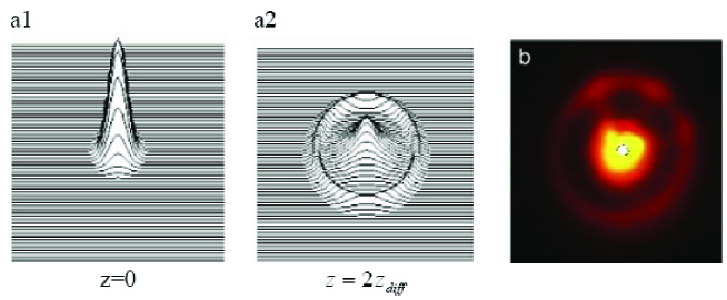
Figure 4: Nonlinear evolution of the waist (intensity) projection $|A(x,y)|^{2}$ of a $400$ $fs$ initial Gaussian pulse (a1) at $\lambda=800$ $nm$, with spot $r_{0}=120$ $\mu m$, and longitudinal spatial pulse duration $z_{0}=v_{gr}t_{0}\cong 120$ $\mu m$ at a distance $z=2z_{diff}$ (a2), obtained by numerical simulation of the 3D+1 nonlinear AE equation (III). The power is above the critical for self-focusing $P=2P_{kr}$ . Typical self-focal zone (core) surrounded by Newton’s ring is obtained. (b) Comparison with the experimental result presented in COU .

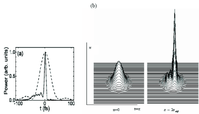
Figure 5: (a) Experimental result of pulse self compression and spliting of the initial pulse to a sequence of several decreasing maxima SKUP . (b) Numerical simulation of the evolution of (x,t=z) projection $|A(x,z^{\prime})|^{2}$ of the same pulse of Fig. 4 at distances $z=0,z=z_{diff}$, governed by the (3D+1) nonlinear AE equation (III) and the ionization-free model.

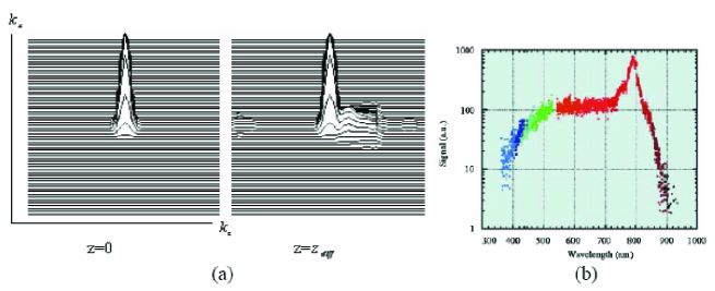
Figure 6: (a) Fourier spectrum of the same side ($x,z$) projection of the intensity $|A(k_{x},k_{z})|^{2}$ as in Fig.5. At one diffraction length the pulse enlarges asymmetrically forwards the short wavelengths (high $k_{z}$ wave-numbers),(b) a spectral form observed also in the experiments COU .

Fig.4 presents the evolution of the spot $|A(x,y|^{2}$ of the initial Gaussian laser pulse at distances $z=0,z=1/2z_{diff},z=z_{diff},z=3/2z_{diff}$. As a result, we obtain the typical self-focal zone (core) with colored ring around, observed in several experiments COU ; KAN ; FAC . The $3D+1$ nonlinear AE equation (III) gives an additional possibility for investigating the evolution of the side projection of the intensity $|A(x,z^{\prime}|^{2}$ profile. The side projection $|A(x,z^{\prime}|^{2}$ of the same pulse is presented in Fig.5. The initial Gaussian pulse begins to self-compress at about one diffraction length and it is split in a sequence of several maxima with decreasing amplitude. Fig. 6 presents the evolution of the Fourier spectrum of the side projection $|A(k_{x},k_{z^{\prime}}|^{2}$. At one diffraction length the pulse enlarges asymmetrically towards the short wavelengths (high wave-numbers). It is important to point here, that similar numerical results for narrow band pulses are obtained when only the self-action term in AE equation (III) is taken into account. The TH or THz term (the second nonlinear term in the brackets) practically does not influence the intensity picture during propagation. In conclusion of this paragraph, we should point out that our non-paraxial ionization-free model (III) and (III) is in good agreement with the experiments on spatial and spectral transformations of a fs pulse in a regime near the critical $P\geq P_{cr}$. Such transformation of the shape and spectrum of the fs pulse is typical in the near zone, up to several diffraction lengths, where the conditions for narrow-band pulse are satisfied $\triangle k_{z}<<k_{0}$.

IV Carrier-to-envelope phase and nonlinear polarization. Drift from THz to GHz generation

In nonlinear regime the spectrum of the amplitude function becomes large due to different nonlinear mechanisms. The Fourier expression $\hat{A}\left[k_{x},k_{y},k_{0}-k_{z},\omega_{0}-\omega\right]$ is a function of arbitrary $\Delta k_{z}=k_{0}-k_{z}$ and $\Delta\omega=\omega_{0}-\omega$, which are related to the group velocity $\Delta\omega/\Delta k_{z}=v_{gr}$ (here, we do not include the nonlinear addition to the group velocity - it is too small for power near the critical one). Let $\Delta k_{z}$ denote an arbitrary initial spectral width of the pulse. In the nonlinear regime $\Delta k_{z}(z)$ enlarges considerably and approaches values $\Delta k_{z}(z)\simeq k_{0}$. To see the difference between the evolution of narrow-band $\Delta k_{z}<<k_{0}$ and broadband $\Delta k_{z}\simeq k_{0}$ pulses, it is convenient to rewrite the amplitude function in Laboratory coordinates (the dispersion number $\beta\simeq 2.1\times 10^{-5}$, being smaller than the diffraction in air, is neglected):

$$A\left(x,y,z,t\right)=B_{0}{B}\left(x,y,z,t\right)\exp{\left(-i(\triangle k_{z}(z-v_{gr}t)\right)},$$ (22)

while in Galilean coordinates it is equal to:

$$V\left(x,y,z^{\prime},t^{\prime}\right)=B_{0}G\left(x,y,z^{\prime},t^{\prime}\right)\exp{\left(-i\triangle k_{z}z^{\prime}\right)}.$$ (23)

The Nonlinear Diffraction Equation (NDE) (III) in Laboratory frame becomes:

$$-2i(k_{0}-\triangle k_{z})\left(\frac{\partial B}{\partial z}+\frac{1}{v_{gr}}\frac{\partial B}{\partial t}\right)=\Delta B-\frac{1}{v_{gr}^{2}}\frac{\partial^{2}B}{\partial t^{2}}+$$

(24)

$$n_{2}k_{0}^{2}B_{0}^{2}\Biggr{\{}\frac{3}{4}|B|^{2}B+\frac{1}{4}\exp{\left[2i\left((k_{0}-\triangle k_{z})z-(k_{0}v_{ph}-v_{gr}\triangle k_{z})t\right)\right]}B^{3}\Biggr{\}}+c.c.,$$

and in Galilean frame, the equation (III) is:

$$-i\frac{2(k_{0}-\triangle k_{z})}{v_{gr}}\frac{\partial G}{\partial t^{\prime}}=\Delta_{\bot}G-\frac{1}{v_{gr}^{2}}\left(\frac{\partial^{2}G}{\partial t^{\prime 2}}-2v_{gr}\frac{\partial^{2}G}{\partial t^{\prime}\partial z^{\prime}}\right)+$$

(25)

$$n_{2}k_{0}^{2}B_{0}^{2}\Biggr{\{}\frac{3}{4}|G|^{2}G+\frac{1}{4}\exp{\left[2i\left((k_{0}-\triangle k_{z})z^{\prime}-k_{0}(v_{ph}-v_{gr})t^{\prime}\right)\right]}G^{3}\Biggr{\}}+c.c.,$$

where $\triangle k_{z}$ can get arbitrary values. It can be seen that the nonlinear phases in both coordinate systems are equal after the transformation $z^{\prime}=z-v_{gr}t;\ t^{\prime}=t$:

$$(k_{0}-\triangle k_{z})z-(k_{0}v_{ph}-\triangle k_{z}v_{gr})t=(k_{0}-\triangle k_{z})z^{\prime}-k_{0}(v_{ph}-v_{gr})t^{\prime}.$$ (26)

On the other hand, the corresponding frequency conversions are different. In Laboratory frame the frequency conversion depends on the spectral width $\triangle k_{z}$:

$$\omega^{Lab}_{nl}=k_{0}v_{ph}-\triangle k_{z}v_{gr},$$ (27)

while in Galilean frame the nonlinear frequency conversion is fixed to the offset frequency

$$\omega^{Gal}_{nl}=k_{0}(v_{ph}-v_{gr})=31GHz;\ (\lambda=800nm)$$ (28)

in air. The expression of the nonlinear frequency shift in Laboratory frame (27) explains the different frequency arising from pulses with different initial spectral width. When the laser is in ns or ps regime, $\triangle k_{z}<<k_{0}$ and the nonlinear frequency shift is equal to the third harmonic $3\omega^{Lab}_{nl}=3\omega_{0}$. In this case (spectral width of the pulse much smaller than the spectral distance to the third harmonic), the phase matching conditions can not be met. Thus, the nonlinear polarization is transformed into a self-action term. The fs pulses on the other hand have initial spectral width of the order $\triangle\omega^{fs}\simeq 10^{13-14}Hz$ and for such pulses at short distances in nonlinear regime the condition $\triangle\omega^{fs}\simeq\omega^{Lab}_{nl}$ can be satisfied. Thus, the nonlinear frequency shift lies within the spectral width of a fs pulse, and from (27) follows the condition for THz and not for TH generation. The self-action enlarges the spectrum up to values $\triangle k_{z}\simeq k_{0}$ and thus, following (27), the nonlinear frequency conversion in far field zone drifts from THz to $\sim 93$ GHz MECH . Note that we consider a single pulse propagation, while the laser system generates a sequences of fs pulses. The different pulses have different nonlinear spectral widths when moving from the source to the far field zone. One would detect in an experiment a mix of frequencies from THz up to GHz.

V Nonlinear sub-cycle regime for $\triangle k_{z}\approx k_{0}$

The separation of the nonlinear polarization to self-action and TH, THz or GHz generated terms is appropriate for fs pulses up to several cycles under envelope. For fs narrow-band pulses, as mentioned in the previous section, the pulse shape is changed by the self-action term, while the CEP frequency depending at the spectral width of the pulse $\triangle k_{z}$ leads to different type of frequency conversion drifts from THz to GHz region. However, when supper-broad spectrum occurs ($\triangle k_{z}\approx k_{0}$), the time width of the pulse $\triangle t$ becomes smaller than the period of the nonlinear oscillation $\omega^{Lab}_{nl}$. In this nonlinear sub-cycle regime, the nonlinear term starts to oscillate with $\omega^{Lab}_{nl}$ and separation of the self-action and the frequency conversion terms becomes mathematically incorrect, due to the mixing of frequencies KOL2 ; KOV2 . For the first time such possibility was discussed in KOL2 , where a correct expression of the nonlinear polarization, including Raman response is presented. In the sub-cycle regime the nonlinear polarization at a fixed frequency and Laboratory frame becomes:

$$n_{2}E^{3}\left(x,y,z,t\right)=n_{2}\exp{\left[i\left((k_{0}-\triangle k_{z})z-(k_{0}v_{ph}-\triangle k_{z}v_{gr})t\right)\right]]}\times$$

(29)

$$\Biggr{\{}\exp{\left[2i\left((k_{0}-\triangle k_{z})z-(k_{0}v_{ph}-\triangle k_{z}v_{gr})t\right)\right]}B^{3}\Biggr{\}},$$

and in Galilean frame it is

$$n_{2}E^{3}\left(x,y,z^{\prime},t^{\prime}\right)=n_{2}\exp{\left[i\left((k_{0}-\triangle k_{z})z^{\prime}-k_{0}(v_{ph}-v_{gr})t^{\prime}\right)\right]]}\times$$

(30)

$$\Biggr{\{}\exp{\left[2i\left((k_{0}-\triangle k_{z})z^{\prime}-k_{0}(v_{ph}-v_{gr})t^{\prime}\right)\right]}B^{3}\Biggr{\}}.$$

In spite of the super-broad spectrum, the dispersion parameter in the transparency region from $400$ $nm$ up to $800$ $nm$ continues to be small, in the range of $\beta\approx 10^{-4}-10^{-5}$. The nonlinear amplitude equations for pulses with super-broad spectrum in Laboratory system become:

$$-2i(k_{0}-\triangle k_{z})\left(\frac{\partial A}{\partial z}+\frac{1}{v_{gr}}\frac{\partial A}{\partial t}\right)=\Delta A-\frac{1}{v_{gr}^{2}}\frac{\partial^{2}A}{\partial t^{2}}+$$

(31)

$$n_{2}k_{0}^{2}\exp{\left[2i\left((k_{0}-\triangle k_{z})z-(k_{0}v_{ph}-\triangle k_{z}v_{gr})t\right)\right]}A^{3},$$

and in Galilean frame

$$-i\frac{(k_{0}-\triangle k_{z})}{v_{gr}}\frac{\partial V}{\partial t^{\prime}}=\Delta_{\bot}V-\frac{1}{v_{gr}^{2}}\left(\frac{\partial^{2}V}{\partial t^{\prime 2}}-2v_{gr}\frac{\partial^{2}V}{\partial t^{\prime}\partial z^{\prime}}\right)+$$

(32)

$$n_{2}k_{0}^{2}\exp{\left[2i\left((k_{0}-\triangle k_{z})z^{\prime}-k_{0}(v_{ph}-v_{gr})t^{\prime}\right)\right]}V^{3}.$$

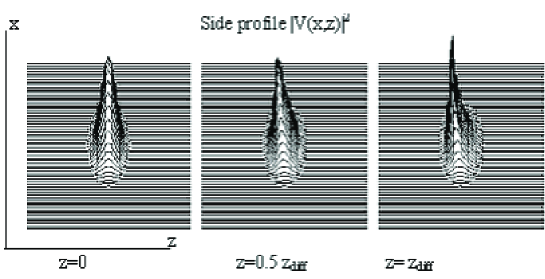
Figure 7: Numerical simulations for an initial Gaussian pulse with super-broad spectrum $\triangle k_{z}\approx k_{0}$ governed by the nonlinear equation (V). The power is slightly above the critical $P=2P_{kr}$. The side projection $|V(x,z^{\prime})|^{2}$ of the intensity is plotted. Instead of splitting into a series of several maxima, the pulse transforms its shape into a Lorentzian of the kind $V(x,y,z^{\prime})\simeq 1/[1+x^{2}+y^{2}+(z^{\prime}+ia)^{2}+a^{2}]$.

Fig. 7 shows a typical numerical solution of the nonparaxial nonlinear equation (V) (or (V)) for an initial Gaussian pulse with super-broad spectrum $\triangle k_{z}\approx k_{0}$. It is obtained by using the split step method ($4$ step Runge-Kutta method for the nonlinear part). These results are the same both in Laboratory and Galilean coordinate frames differing only by a translation. The side projection $|V(x,z^{\prime}|^{2}$ of the intensity profile is plotted for different propagation distances. Instead of splitting into to a series of several maxima, the pulse transforms its shape in a Lorentzian type form of the kind $V(x,y,z)\simeq 1/[1+x^{2}+y^{2}+(z^{\prime}+ia)^{2}+a^{2}]$. Here, the number $a$ accounts for compression in $z^{\prime}$ direction and a spatial angular distribution. Fig. 8 presents the evolution of the spectrum $|V(k_{x},k_{z^{\prime}}|^{2}$ of the side intensity projection for the same pulse. The spectrum enlarges forwards the small $k_{z}$ wave-numbers (long wavelengths) - typical for Lorentzian type profiles. To compare with Fig. 8, Fig. 9 gives a plot of the side projection $|V(k_{x},k_{z}^{\prime}|^{2}$ of the spectrum of a Lorentzian profile $V(x,y,z^{\prime})=1/[1+x^{2}+y^{2}+(z^{\prime}+ia)^{2}+a^{2}]$, $a=2$ increases toward the small wave-numbers. The numerical experiments lead to the conclusion that a possible shape of the stable $3D+1$ soliton can be in the form of a Lorentzian profile. Thus, if we take as an initial condition Lorentzian, instead Gaussian one, a relative stability in the shape and spectrum can be expected. Fig. 10 shows the evolution of the $|V(x,z^{\prime}|^{2}$ profile of a pulse with initial Lorentzian shape $V(x,y,z^{\prime},t=0)=1/[1+x^{2}+y^{2}+(z^{\prime}+ia)^{2}+a^{2}]$, $a=2$. The pulse propagates at distance of one diffraction length, preserving its initial shape.

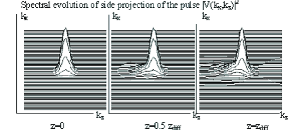
Figure 8: The evolution of the spectrum $|V(k_{x},k_{z})|^{2}$ of the same side intensity projection $|V(x,z^{\prime})|^{2}$ . The spectrum enlarges towards small $k_{z}$ wave-numbers (long wavelengths) - typical for Lorentzian profiles.

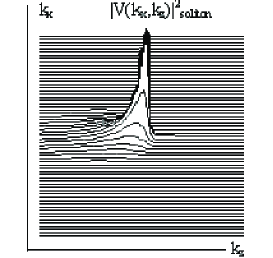
Figure 9: Plot of the side projection $|V(k_{x},k_{z}|^{2}$ of the spectrum of a Lorentzian profile $V(x,y,z)=1/[1+x^{2}+y^{2}+(z+ia)^{2}+a^{2}]$, $a=2$ increasing towards the small $k_{z}$ wave-numbers (compare with Fig. 8).

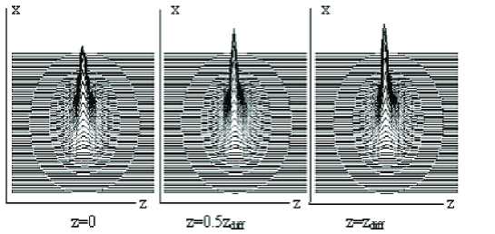
Figure 10: Evolution of the $|V(x,z^{\prime}|^{2}$ profile of a pulse with super-broad spectrum $\triangle k_{z}\approx k_{0}$ and initial Lorentzian shape $V(x,y,z^{\prime},t=0)=1/([1+x^{2}+y^{2}+(z^{\prime}+ia)^{2}+a^{2}$], $a=2$, governed by the nonlinear equation (V). The pulse propagates over one diffraction length with relatively stable form.

VI Spectrally asymmetric 3D+1 soliton solution

The numerical simulations in the previous section for broad band spectrum pulses demonstrate a stable soliton propagation with a specific initial Lorentzian shape. To find an exact soliton solution, we require that $\triangle k_{z}=k_{0}$ and $\triangle\omega\cong\omega_{0}$ be satisfied. In air $\beta\cong 0$ and the amplitude equation (V) can be rewritten as:

$$\Delta B-\frac{1}{v_{gr}^{2}}\frac{\partial^{2}B}{\partial t^{2}}+k_{0}^{2}n_{2}B_{0}^{2}\exp{\left[i\left(2\triangle\omega_{nl}t\right)\right]}B^{3}=0.$$ (33)

To minimize the influence of the GHz oscillation $\omega_{nl}$, we use an amplitude function with a phase opposite to CEP:

$$B(x,y,x,t)=C(x,y,z,t)\exp(-i\triangle\omega_{nl}t).$$ (34)

This corresponds to an oscillation of our soliton solution with frequency $\omega_{nl}\simeq 31$ GHz. The equation (33) becomes:

$$\Delta C-\frac{1}{v_{gr}^{2}}\frac{\partial^{2}C}{\partial t^{2}}+k_{0}^{2}n_{2}B_{0}^{2}C^{3}=2i\frac{\triangle\omega_{nl}}{v_{gr}^{2}}\frac{\partial C}{\partial t}-\frac{\triangle\omega_{nl}^{2}}{v_{gr}^{2}}C$$ (35)

To estimate the influence of the different terms on the propagation dynamics we rewrite equation (35) in dimensionless form. Substituting:

$$t=t_{0}t;\ z=z_{0}z;\ x=r_{0}x;\ y=r_{0}y;$$ (36)

$$r_{0}/z_{0}=\delta\sim 1;\ z_{0}=v_{gr}t_{0};\ t_{0}\cong 2\times 10^{-13}-10^{-14}sec,$$ (37)

we obtain the following normalized equation:

$$\Delta C-\frac{\partial^{2}C}{\partial t^{2}}+\gamma C^{3}=i\alpha\frac{\partial C}{\partial t}-\beta C,$$ (38)

where $\gamma=r_{0}^{2}k_{0}^{2}n_{2}B_{0}^{2}$ is the nonlinear constant, $\alpha=2\triangle\omega_{nl}r_{0}^{2}/v_{gr}^{2}t_{0}$ and $\beta=\triangle\omega_{nl}^{2}r_{0}^{2}/v_{gr}^{2}$. For typical fs laser pulse at carrier wavenumber $800$ $nm$ with spot $r_{0}=100$ $\mu m$, the constants of both terms in the r.h.s of equation (38) are very small ($\alpha\sim 10^{-2}$ and $\beta\sim 10^{-4}$) and can be neglected. Thus, equation (38) becomes:

$$\Delta C-\frac{\partial^{2}C}{\partial t^{2}}+\gamma C^{3}=0.$$ (39)

Furthermore, we shall assume that the new envelope wave equation (39) has solutions in the form:

$$C\left(x,y,z,t\right)=C(\tilde{r}),$$ (40)

where $\tilde{r}=\sqrt{x^{2}+y^{2}+(z+ia)^{2}-(t+ia)^{2}}$. From the nonlinear wave equation (39), using (40), the following ordinary nonlinear equation is obtained:

$$\frac{3}{\tilde{r}}\frac{\partial C}{\partial\tilde{r}}+\frac{\partial^{2}C}{\partial\tilde{r}^{2}}+\gamma C^{3}=0.$$ (41)

The number $a$ counts for the longitudinal compression and the phase modulation of the pulse. When the nonlinear coefficient is slightly above the critical and reaches the value $\gamma=2$, equation (41) has exact particle-like solution of the form:

$$C=\frac{sech(ln(\tilde{r}))}{\tilde{r}}.$$ (42)

Using the fact that $exp(ln(\tilde{r}))=\tilde{r}$ and $exp(-(ln\tilde{r}))=\frac{1}{\tilde{r}}$, the solution (42) is simplified to the following algebraic soliton:

$$C(\tilde{r})=\frac{2}{1+x^{2}+y^{2}+(z+ia)^{2}-(t+ia)^{2}}$$ (43)

The solution (43) gives the time evolution of our Lorentz initial form, investigated in the previous section. As be seen from equation (39), the solution appears as a balance between the parabolic (not paraxial) wave type diffraction of broad band pulse $\triangle k_{z}=k_{0}$ and the nonlinearity of third order. The maxima of this solution are at the points where $\tilde{r}^{2}=0$. If we turn back to standard, not normalized coordinates, and solve the second order equation $z^{2}+2iaz-2iav_{gr}t-v_{gr}^{2}t^{2}=0$, only one real solution $z=v_{gr}t$ can be obtained. It corresponds to one-directional propagation with position of the maximum on the $z$ - coordinate $z=v_{gr}t$. As it was pointed above, Fig. 8 presents the initial $k_{x},k_{z}$ spectrum of the soliton (43). While the $k_{x},k_{y}$ spectrum is symmetric, the $k_{z}$ projection is fully asymmetric, enlarging forwards to low $k_{z}$ wave-numbers (long wavelengths), and has typical Lorentz shape. Recently, in experiments with $2-3$ cycle pulses long range filaments with similar spectral profile KOVACEV are observed. We suppose that in this experiment a $3D+1$ Lorentz type soliton was found experimentally for the first time.

VII Conclusions

In this paper we investigate femtosecond pulse propagation in air, governed by the AE equation, in linear and nonlinear regime. The equation allows to solve the problem of propagation of pulses with super-broad spectrum. Note that this problem can not be studied in paraxial optics. In linear regime the fundamental solutions of AE (1) and DE (2) are obtained and different regimes of diffraction are analyzed. The typical fs pulses up to $50$ fs diffract by the Fresnel law, in a plane orthogonal to the direction of propagation, while their longitudinal shape is preserved in air or is enlarged a little, due to the dispersion. Broad-band pulses (only a few cycles under envelope) at several diffraction lengths diffract in a parabolic form. We solve the convolution problem of the diffraction equation DE (2) for an initial pulse in the form of a Gaussian bullet, and obtain an exact analytical solution (II). A new method for solving evolution problems of the wave equation is also suggested. We investigate precisely the nonlinear third order polarization, including the CEP into account. This additional phase transforms TH term to THz or GHz terms, depending on the spectral width of the pulse. Thus, we suggest a new mechanism of THz and GHz generation from fs pulses in nonlinear regime. For pulses with power a little above the critical for self-focusing, we investigate two basic cases: pulses with narrow-band spectrum and with broad-band spectrum. The numerical simulation of the evolution of narrow-band pulses (standard $100$ fs pulses), gives a typical conical emission and a spectral enlargement to the short wavelengths. Our study of broad-band pulses leads to the conclusion that their propagation is governed by the nonlinear wave equation with third order nonlinear term (39), when the THz oscillation is neglected as small term. An exact soliton solution of equation (39), with $3D+1$ Lorentz shape is also obtained. The soliton appears as a balance between parabolic divergent type diffraction and parabolic convergent type of nonlinear self-focusing. Numerically, we demonstrate a relative stability of the soliton pulse with respect to the THz oscillations.

VIII Acknowledgements

This work is partially supported by the Bulgarian Science Foundation under grant DO-02-0114/2008.

IX List of Figure Captions

Fig.1 Plot of the waist (intensity’s) projection $|A(x,y)|^{2}$ of a $100$ $fs$ Gaussian pulse at $\lambda=800$ $nm$, with initial spot $r_{0}=60$ $\mu m$, and longitudinal spatial pulse duration $z_{0}=30$ $\mu m$, as solution of the linear equation in local time (12) on distances expressed by diffraction lengths. The spot deformation satisfies the Fresnel diffraction law and on one diffraction length $z=z_{diff}$ the diameter of the spot increases twice, while the maximum of the pulse decreases with the same factor.

Fig. 2 Side ($x,\tau$) projection of the intensity $|A(x,\tau)|^{2}$ for the same optical pulse as in Fig. 1. The ($x,y$) projection of the pulse diffracts considerably following the Fresnel law, while the ($\tau$) projection on several diffraction lengths preserves its initial shape due to the small dispersion. The diffraction - dispersion picture, presented by the side $(x,\tau)$ projection, gives idea of what should happen in the nonlinear regime: the plane wave diffraction with a combination of parabolic type nonlinear Kerr focusing always leads to self-focusing for narrow-band ($\triangle k_{z}<<k_{0}$) pulses.

Fig. 3 Side ($x,z$) projection of the intensity $|A(x,z^{\prime})|^{2}$ for a normalized $10$ fs Gaussian initial pulse at $\lambda=800$ nm, $\triangle k_{z}\simeq k_{0}/3$, $z_{0}=r_{0}/2$, and only $3$ cycles under the envelope (large-band pulse $\triangle k_{z}\approx k_{0}$), obtained numerically from the AE equation (8) in Galilean frame. At $3$ diffraction lengths a divergent parabolic type diffraction is observed. In nonlinear regime a possibility appear: the divergent parabolic type diffraction for large-band pulses to be compensated by the converged parabolic type nonlinear Kerr focusing.

Fig. 4 Nonlinear evolution of the waist (intensity) projection $|A(x,y)|^{2}$ of a $400$ $fs$ initial Gaussian pulse (a1) at $\lambda=800$ $nm$, with spot $r_{0}=120$ $\mu m$, and longitudinal spatial pulse duration $z_{0}=v_{gr}t_{0}\cong 120$ $\mu m$ at a distance $z=2z_{diff}$ (a2), obtained by numerical simulation of the 3D+1 nonlinear AE equation (III). The power is above the critical for self-focusing $P=2P_{kr}$ . Typical self-focal zone (core) surrounded by Newton’s ring is obtained. (b) Comparison with the experimental result presented in COU .

Fig. 5 (a) Experimental result of pulse self compression and spliting of the initial pulse to a sequence of several decreasing maxima SKUP . (b) Numerical simulation of the evolution of (x,t=z) projection $|A(x,z^{\prime})|^{2}$ of the same pulse of Fig. 4 at distances $z=0,z=z_{diff}$, governed by the (3D+1) nonlinear AE equation (III) and the ionization-free model.

Fig. 6 (a) Fourier spectrum of the same side ($x,z$) projection of the intensity $|A(k_{x},k_{z})|^{2}$ as in Fig.5. At one diffraction length the pulse enlarges asymmetrically forwards the short wavelengths (high $k_{z}$ wave-numbers),(b) a spectral form observed also in the experiments COU .

Fig.7 Numerical simulations for an initial Gaussian pulse with super-broad spectrum $\triangle k_{z}\approx k_{0}$ governed by the nonlinear equation (V). The power is slightly above the critical $P=2P_{kr}$. The side projection $|V(x,z^{\prime})|^{2}$ of the intensity is plotted. Instead of splitting into a series of several maxima, the pulse transforms its shape into a Lorentzian of the kind $V(x,y,z^{\prime})\simeq 1/[1+x^{2}+y^{2}+(z^{\prime}+ia)^{2}+a^{2}]$.

Fig. 8 The evolution of the spectrum $|V(k_{x},k_{z})|^{2}$ of the same side intensity projection $|V(x,z^{\prime})|^{2}$ . The spectrum enlarges towards small $k_{z}$ wave-numbers (long wavelengths) - typical for Lorentzian profiles.

Fig. 9 Plot of the side projection $|V(k_{x},k_{z}|^{2}$ of the spectrum of a Lorentzian profile $V(x,y,z)=1/[1+x^{2}+y^{2}+(z+ia)^{2}+a^{2}]$, $a=2$ increasing towards the small $k_{z}$ wave-numbers (compare with Fig. 8).

Fig. 10 Evolution of the $|V(x,z^{\prime}|^{2}$ profile of a pulse with super-broad spectrum $\triangle k_{z}\approx k_{0}$ and initial Lorentzian shape $V(x,y,z^{\prime},t=0)=1/([1+x^{2}+y^{2}+(z^{\prime}+ia)^{2}+a^{2}$], $a=2$, governed by the nonlinear equation (V). The pulse propagates over one diffraction length with relatively stable form.

References

- (1) A. Braun, G. Korn, X. Liu, D. Du, J. Squier, and G. Mourou, ”Self-channeling of high-peak-power femtosecond laser pulses in air”, Opt. Lett. , 20(1), 73-75 (1995).
- (2) L. Wöste, C. Wedekind, H. Wille, P. Rairoux, B. Stein, S. Nikolov, C. Werner, S.Nierdermeier, F. Ronneberger, H. Schillinger, and R. Sauerbrey, ”Femtosecond atmospheric lamp”, AT-Fachverlag, Stuttgard, Laser and Optoelectronik 29, 51-53 (1997).
- (3) G. Méchain, C. D’Amico, Y.-B. André, S. Tzortzakis, M. Franco, B. Prade, A. Mysyrowicz, A. Couairon, E. Salmon, R. Sauerbrey, ”Length of plasma filaments created in air by a multiterawatt femtosecond laser”, Opt. Commun. , 247, 171-108 (2005).
- (4) S. Tzortzakis, G. Méchain, G. Patalano, Y.-B. André, B. Prade, M. Franco, A. Mysyrowicz, J. M. Munier, M. Gheudin, G. Beaudin, and P. Encrenaz, ”Coherent subterahertz radiation from femtosecond infrared filaments in air”, Opt. Lett. , 1944-1946, (2002).
- (5) C. D’Amico, A. Houard, M. Franco, B. Prade, A. Mysyrowicz, ”Coherent and incoherent THz radiation emission from femtosecond filaments in air”, Optics Express, 15, 15274-15279 (2007).
- (6) C. D’Amico, A. Houard, S. Akturk, Y. Liu, J. Le Bloas, M. Franco, B. Prade, A. Couairon, V. T. Tikhonchuk, and A. Mysyrowicz, ”Forward THz radiation emission by femtosecond filamentation in gases: theory and experiment”, New J. of Phys., 10, 013015 (2008).
- (7) C. P. Hauri, W. Kornelis, F. W. Helbing, A. Couairon, A. Mysyrowicz, J. Biegert, U. Keller, ”Generation of intense, carrier-envelope phase locked few-cycle laser pulses through filamentation”, Appl. Phys. B, 79, 673-677 (2004).
- (8) C. P. Hauri, A. Guandalini, P. Eckle, W. Kornelis, J. Biegert, U. Keller. ”Generation of intense few cycle laser pulses through filamentation - parameter dependence”, Optics Express, 13, 7541 (2005).
- (9) A. Couairon, J. Biegert, C. P. Hauri, W. Kornelis, F. W. Helbing, U. Keller, A. Mysyrowicz, ”Self-compression of ultrashort laser pulses down to one optical cycle by filamentation”, J. Mod. Opt., 53, 75-85 (2006).
- (10) S.L. Chin, A. Brodeur, S. Petit, O. G. Kosareva, V. P. Kandidov, ” Filamentation and supercontituum generation during the propagation of powerful ultrashort laser pulses in optical media (white light laser)”, J. Nonlinear Opt. Phys. Mater., 8, 121-146 (1998).
- (11) J. Kasparian, R. Sauerbrey, D. Mondelain, S. Niedermeier, J. Yu, Y. P. Wolf, Y.-B. André, M. Franco, B. S. Prade, S. Tzortzakis, A. Mysyrowicz, H. Wille, M. Rodriguez, L. Wöste, ”Infrared extenstion of the supercontinuum generated by femtosecond terrawattlaser pulses propagating in the atmosphere”, Opt. Lett. , 25, 1397-1399 (2000).
- (12) A. Couairon, and A. Mysyrowicz, ”Femtosecond filamentation in transparent media”, Physics Reports, 441, 47-189 (2007).
- (13) S. L. Chin, S. A. Hosseini, W. Liu, Q. Luo, F. Théberge, N. Aközbek, A. Becker, V. P. Kandidov, O. G. Kosareva, and H. Schoeder, ”The propagation of powerful femtosecond laser pulses in optical media: physics, applications, and new challenges”, Can. J. Phys. 83, 863-905 (2005).
- (14) Daniele Faccio, Alessandro Averhi, Antonio Lotti, Paolo Di Trapani, Arnaud Couairon, Dimitris Papazoglou, Stelios Tzortzakis, ”Ultrashort laser pulse filamentation from spontaneous X Wave formation in air”, Optics Express, 16 1565-1569 (2008)
- (15) M. Kolesik and J. V. Moloney, ”Perturbative and non-perturbative aspects of optical filamentation in bulk dielectric media.”, Optics Express, 16, 2971-2986 (2008).
- (16) Y. R. Shen, The Principles of Nonlinear Optics, Wiley-Interscience, New York, 1984.
- (17) P. Béjot, J. Kasparian, S. Henin, V. Loriot, T. Viellard, E. Hertz, O. Faucher, B. Lavorel, and J.-P. Wolf, ”Higher-Order Kerr Terms Allow Ionization-Free Filamentation in Gases”, Phys. Rev. Lett., 104, 103903 (2010).
- (18) G. Méchain, A. Couairon, Y.-B. André, C. D’Amico, M. Franco, B. Prade, S. Tzortzakis, A. Mysyrowicz, R. Sauerbrey, ”Long-range self-channeling of infrared laser pulses in air: a new regime without ionization”, Appl. Phys B, 79, 379-382 (2004).
- (19) A. Dubietis, E. Gaižauskas, G. Tamožauskas, P. Di Trapani, ”Light filaments without self-channeling”, Phys. Rev. Lett 92, 253903 (2004).
- (20) Todd A. Pitts, Ting S. Luk, James K. Gruetzner, Thomas R. Nelson, Armon McPherson, Stewart M. Cameron and Aaron C. Bernstein, ”Propagation of self-focused laser pulse in atmosphere: experiment versus numerical simulation”, J. Opt. Soc. Am. B, 21, 2006-2016 (2004).
- (21) Martin Wegener, Extreme Nonlinear Optics, (Springer-Verlag, Berlin Heidelberg, 2005).
- (22) A. Hasegawa, Optical Solitons in Fibers, (Springer, Berlin,1989).
- (23) G. P. Agrawal, Nonlinear Fiber Optics, (Academic, San Diego, 2001).
- (24) E. M. Dianov, P.V. Mamyshev, A. M. Prokhorov, and V. N. Serkin, Nonlinear Effects in Fibers, (Harwood Academic, NewYork, 1989).
- (25) V. N. Serkin, A. Hasegawa, and T. L. Belyaeva, ”Nonautonomous Solitons in External Potentials”, Phys. Rev. Lett. 98, 074102 (2007).
- (26) Lubomir M. Kovachev, Kamen Kovachev, ”Diffraction of femtosecond pulses: nonparaxial regime”,J. Opt. Soc. Am. A, 25, 2232-2243 (2008); ”Erratum ”, 25, 3097-3098 (2008).
- (27) I. P. Christov, ”Propagation of femtosecond light pulses”, Opt. Comm., 53, 364-366 (1985).
- (28) T. Brabec, F. Krausz, ”Nonlinear Optical Pulse Propagation in the Single-Cycle Regime”, Phys. Rev. Lett. 78, 3282-3285 (1997).
- (29) A. P. Kiselev, ”Localized Light Waves: Paraxial and Exact Solutions of the Wave Equation”, Optics and Spectroscopy, 102, 603-622 (2007).
- (30) Stefan Skupin, Gero Stibenz, Luc Berge, Falk Lederer, Thomas Sokollik, Matthias Schnurer, Nickolai Zhavoronkov, and Gunter Steinmeyer ,”Self-compression by femtosecond pulse filamentation: Experiments versus numerical simulations” Phys. Rev. E 74, 056604 (2006).
- (31) J. Kasparian, R. Sauerbrey, and S. L. Chin, ”The critical laser intensity of self-guided light filaments in air”, Appl. Phys. B 71, 877-879 (2000).
- (32) M. Kolesik, E. M. Wright, A. Becker, and J. V. Moloney, ”Simulation of third-harmonic and supercontinuum generation for femtosecond pulses in air”, Appl. Phys. B, 85, 531-538 (2006).
- (33) L. M. Kovachev, ”New mechanism for THz oscillation of the nonlinear refractive index in air: particle-like solutions”, J. Mod. Opt., 56, 1797 - 1803 (2009).
- (34) E. Schulz and M. Kovacev, private communication.