Arrangement Computation for Planar Algebraic Curves

Abstract

We present a new certified and complete algorithm to compute arrangements of real planar algebraic curves. Our algorithm provides a geometric-topological analysis of the decomposition of the plane induced by a finite number of algebraic curves in terms of a cylindrical algebraic decomposition of the plane. Compared to previous approaches, we improve in two main aspects: Firstly, we significantly reduce the amount of exact operations, that is, our algorithms only uses resultant and $\gcd$ as purely symbolic operations. Secondly, we introduce a new hybrid method in the lifting step of our algorithm which combines the usage of a certified numerical complex root solver and information derived from the resultant computation. Additionally, we never consider any coordinate transformation and the output is also given with respect to the initial coordinate system.

We implemented our algorithm as a prototypical package of the C++-library Cgal. Our implementation exploits graphics hardware to expedite the resultant and $\gcd$ computation. We also compared our implementation with the current reference implementation, that is, Cgal’s curve analysis and arrangement for algebraic curves. For various series of challenging instances, our experiments show that the new implementation outperforms the existing one.

1 Introduction

Computing the topology of a planar algebraic curve

$$C=V(f)=\{(x,y)\in\mathbb{R}^{2}:f(x,y)=0\}$$ (1.1)

can be considered as one of the fundamental problems in real algebraic geometry with numerous applications in computational geometry, computer graphics and computer aided geometric design. Typically, the topology of $C$ is given in terms of a planar graph $\mathcal{G}_{C}$ isotopic to $C$. For a geometric-topological analysis, we further require the vertices of $\mathcal{G}_{C}$ to be located on $C$. In this paper, we study the general problem of computing an arrangement of a given set of algebraic curves, that is, the decomposition of the plane into cells of dimensions $0$, $1$ and $2$ induced by the given curves. The proposed algorithm is certified and complete, and the overall arrangement computation is exclusively carried out in the initial coordinate system. Efficiency of our approach is shown by implementing our algorithm and comparing it to the current reference implementation.

There exist a number of certified and complete approaches to determine the topology of an algebraic curve; we refer the reader to [12, 18, 23, 25, 29] for recent work and further references. At present, only the method from [18] has been extended to arrangement computations of arbitrary algebraic curves [17]. Common to all existing approaches is that, in a first step, they use eliminations techniques (e.g., resultants) to project the $x$-critical points (i.e., points $p\in C$ with $f_{y}(p)=0$) of the curve into one dimension. In a second step, the fiber at each of these projected points is computed. In general, this lifting step has turned out to be the most time-consuming part because it amounts to determining the real roots of a non-square univariate polynomial $f(\alpha,y)\in\mathbb{R}[y]$ with algebraic coefficients. The high computational cost for computing the roots of $f(\alpha,y)$ is mainly due to a more comprehensive algebraic machinery such as subresultants (in [17, 18, 23]), Gröbner basis or rational univariate representation (in [12]) in order to obtain additional information on the number of distinct real (or complex) roots of $f(\alpha,y)$ or the multiplicity of the multiple roots of $f(\alpha,y)$. In addition, all except the method from [12] consider a shearing of the curve which guarantees that the sheared curve has no two $x$-critical points sharing the same $x$-coordinate which in turn simplifies the lifting step but for the price of giving up sparseness of the initial input; an approach, which usually results in larger bitsizes of the coefficients and considerably increased running times. In a final connection step, arcs adjacent to the same $x$-critical points are identified.

The high-level description of the algorithm presented in this paper is almost identical to that of the existing methods, and, similar as in [17, 18], we reduce the arrangement computation to the geometric-topological analysis of a single curve and of a pair of curves. However, we improve in the following two main aspects: Firstly, we considerably reduce the amount of purely symbolic computations, that is, we only use resultant and $\gcd$ computation. The main reason for this approach is that we can outsource both computations to graphics hardware [20, 21, 22], removing a bottleneck of previous methods which was due to the high amount of symbolic operations. Secondly, for curve analysis, we use a result from Teissier [24, 33] to obtain additional information for the number of distinct complex roots of $f(\alpha,y)$ along a critical fiber (actually, an upper bound which most likely matches the exact number). We combine this information with a new certified complex root solver [26] to isolate the roots of $f(\alpha,y)$. The latter symbolic-numeric step applies as an efficient filter denoted FastLift which fails only for very special instances. In order to achieve completeness of our overall method (i.e., for cases where FastLift fails), we modify the method from [4] for solving bivariate polynomial systems in order to isolate the roots of $f(\alpha,y)$.

We implemented our algorithm as a development branch of Cgal’s bivariate algebraic kernel (Ak_2 for short) which is based on the algorithms from [17, 18] for topology and arrangement computation. Intensive benchmarks [18, 29] have shown that Ak_2 can be considered as the current reference implementation. For fair comparison, we run an Ak_2 with GPU-enabled resultants and $\gcd$s against our implementation on numerous challenging benchmark instances. Our experiments show that the new approach outperforms Ak_2 for all instances. More precisely, our method is, on average, twice as fast for easy instances such as non-singular curves in generic position. For hard instances, we typically improve by large factors between $5$ and $120$ which is mainly due to the new symbolic-numeric filter FastLift, the exclusive usage of resultant and $\gcd$ as only symbolic operations and the abstinence of shearing. In summary, the presented approach demonstrates the strength of symbolic-numeric techniques. It further proves that, in order to achieve efficiency in an actual implementation, it is of great importance to reduce the amount of symbolic operations and to consider approximate operations whenever this is possible.

Finally, we are confident that our new approach will have some positive impact in the following respects: Existing subdivision methods [2, 11, 28] show excellent behavior for non-singular input. For singular input, they can be made certifying and complete when considering worst case separation bounds, however, this approach has not shown effective in practice so far. Another advantage of subdivision methods compared to elimination approaches is that they are local and do not need (global) algebraic operations. In our method, we considerably reduced the amount of such algebraic operations and outsourced the remaining computations to graphics card. Hence, it seems reasonable that combining our algorithm with a subdivision approach eventually leads to a certified and complete method which shows excellent “local” behavior as well. We further see numerous applications of our method, in particular, when computing arrangements of surfaces. The actual implementation [7] for surface triangulation is crucially based on planar arrangement computations of singular curves. Thus, we are confident to considerably improve its efficiency based on the new algorithm for planar arrangement computation.

2 Curve Analysis

2.1 The Algorithm

The input of our algorithm is a planar algebraic curve $C$ as defined in (1.1), where $f$ is a square-free, bivariate polynomial $f\in\mathbb{Z}[x,y]$ with integer coefficients. If $f$ is considered as polynomial in $y$ with coefficients $f_{i}(x)\in\mathbb{Z}[x]$, its coefficients typically share a trivial content $h:=\gcd(f_{0},f_{1},\ldots)$. A non-trivial content $h\notin\mathbb{Z}$ defines vertical lines at the real roots of $h$. Our algorithm handles this situation by dividing out $h$ first and finally merging the vertical lines defined by $h=0$ and the curve analysis of the curve $C^{\prime}:=V(f/h)$. Hence, throughout the following considerations, we can assume that $h$ is trivial, thus $C$ contains no vertical line.

The algorithm returns a planar graph $\mathcal{G}_{C}$ that is isotopic to $C$, where all vertices $V$ of $\mathcal{G}_{C}$ are located on $C$. The proposed algorithm follows a classical cylindrical algebraic decomposition approach. We start with a high-level description of the three-step algorithm.

In the first step, the projection phase, we project all $x$-critical points $(\alpha,\beta)\in C$ (i.e., $f(\alpha,\beta)=f_{y}(\alpha,\beta)=0$) onto the $x$-axis by means of a resultant computation and root isolation for the elimination polynomial. The set of $x$-critical points comprises exactly the points where $C$ has a vertical tangent or is singular. It is well known (e.g., see [25, Theorem 2.2.10] for a short proof) that, for any two consecutive $x$-critical values $\alpha$ and $\alpha^{\prime}$, $C$ is delineable over $I=(\alpha,\alpha^{\prime})$, that is, $C|_{I\times\mathbb{R}}$ decomposes into a certain number $m_{I}$ of disjoint function graphs $C_{I,1},\ldots,C_{I,m_{I}}$. In the lifting phase, we first isolate the roots of the (square-free) intermediate polynomial $f(q_{I},y)\in\mathbb{Q}[y]$, where $q_{I}$ constitutes an arbitrary chosen but fixed rational value in $I$. This computation yields the number $m_{I}$ ($=$ number of real roots of $f(q_{I},y)$) of arcs above $I$ and corresponding representatives $(q_{I},y_{I,i})\in C_{I,i}$ on each arc. We further compute all points on $C$ that are located above an $x$-critical value $\alpha$, that is, we determine the real roots $y_{\alpha,1},\ldots,y_{\alpha,m_{\alpha}}$ of each (non square-free) fiber polynomial $f(\alpha,y)\in\mathbb{R}[y]$. From the latter two computations, we obtain the vertex set $V$ of $\mathcal{G}_{C}$ as the union of all points $(q_{I},y_{I,i})$ and $(\alpha,y_{\alpha,i})$. In the final connection phase, which concludes the topology analysis, we determine which of the above vertices are connected via an arc of $C$. For each connected pair $(v_{1},v_{2})\in V$, we insert a line segment connecting $v_{1}$ and $v_{2}$. It is then straightforward to prove that $\mathcal{G}_{C}$ is isotopic to $C$; see [25, Theorem 6.4.4] for a proof. We remark that we never consider any kind of coordinate transformation, even in case where $C$ contains two or more $x$-critical points sharing the same $x$-coordinate.

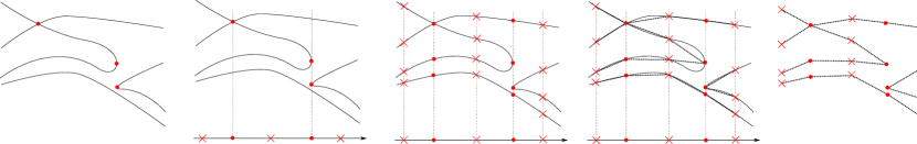
Figure 2.1: The figure on the left shows a curve $C$ with two $x$-extremal points and one singular point (red dots). In the projection phase, these points are projected onto the $x$-axis and rational points separating the $x$-critical values are inserted (red crosses). In the lifting phase, the fibers at the critical values (red dots) and at the rational points in between (red crosses) are computed. In the connection phase, each pair of lifted points connected by an arc of $C$ is determined and a corresponding line segment is inserted. The right figure shows the final graph that is isotopic to $C$.

We next describe the three phases in detail:

2.1.1 Projection Phase

In the projection step, we follow well-known techniques from elimination theory, that is, we compute the resultant $R(x):=\operatorname{res}(f,f_{y},y)\in\mathbb{Z}[x]$ and a square-free factorization of $R$. More precisely, we determine square-free and pairwise coprime factors $r_{i}\in\mathbb{Z}[x]$, $i=1,\ldots,\deg(R)$, such that $R(x)=\prod_{i=1}^{\deg(R)}\left(r_{i}(x)\right)^{i}$. We remark that, for some $i\in\{1,\ldots,\deg(R)\}$, $r_{i}(x)\equiv 1$. Yun’s algorithm [35, Alg. 14.21] constructs such a square-free factorization by essentially computing greatest common divisors of $R$ and its higher derivatives in an iterative way. Next, we isolate the real roots $\alpha_{i,j}$, $j=1,\ldots,\ell_{i}$, of the polynomials $r_{i}$ which in turn are $i$-fold roots of $R$. More precisely, we compute disjoint intervals $I(\alpha_{i,j})\subset\mathbb{R}$ with rational endpoints such that $I(\alpha_{i,j})$ contains $\alpha_{i,j}$ but no other root of $r_{i}$, and the union of all $I(\alpha_{i,j})$, $j=1,\ldots,\ell_{i}$, contains all real roots of $r_{i}$. For the real root isolation, we consider the Descartes method [15, 30] as a suited algorithm. By further refining the isolating intervals, we can achieve that all intervals $I(\alpha_{i,j})$ are pairwise disjoint and, thus, also constitute isolating intervals for the real roots of $R$. Then, for each pair $\alpha$ and $\alpha^{\prime}$ of consecutive roots of $R$ defining an open interval $I=(\alpha,\alpha^{\prime})$, we choose a separating rational value $q_{I}$ in between the corresponding isolating intervals.

2.1.2 Lifting Phase

Isolating the roots of the intermediate polynomials $f(q_{I},y)$ is rather straightforward: since $f(q_{I},y)$ is a square-free polynomial with rational coefficients, the Descartes method directly applies. Determining the roots of $f(\alpha,y)\in\mathbb{R}[y]$ at an $x$-critical value $\alpha$ is more complicated because $f(\alpha,y)$ has multiple roots and, in general, irrational coefficients. We propose to run the following approach: We first consider a method denoted FastLift which works as a filter for the fiber computation. We will see in the experiments enlisted in Section 4 that FastLift applies to all fibers for the majority of all input curves and only fails for a small number of fibers for some very special instances. In case of success, the fiber at $\alpha$ is returned. If FastLift fails, we use a second method denoted Lift which serves as a ”backup” for FastLift. In comparison to FastLift, Lift is a complete method which applies to any input curve and any corresponding $x$-critical value, however, for the price of being less efficient. Nevertheless, our experiments show that even the exclusive use of Lift significantly improves upon existing approaches.

Lift — a complete method for fiber computation: Lift is based on our recent studies on solving a bivariate polynomial system. In [4], we introduced a highly efficient method, denoted Bisolve, to isolate the real solutions of a system of two bivariate polynomials $f,g\in\mathbb{Q}[x,y]$. Its output consists of a set of disjoint boxes $B_{1},\ldots,B_{m}\subset\mathbb{R}^{2}$ such that each box $B_{i}$ contains exactly one real solution $\xi:=(x_{0},y_{0})$ of $f(x,y)=g(x,y)=0$, and the union of all $B_{i}$ covers all solutions. Furthermore, for each solution $\xi$, Bisolve provides square-free polynomials $p,q\in\mathbb{Z}[x]$ with $p(x_{0})=q(y_{0})=0$ and corresponding isolating (and refineable) intervals $I(x_{0})$ and $I(y_{0})$ for $x_{0}$ and $y_{0}$, respectively. Comparing $\xi$ with another point $\xi_{1}=(x_{1},y_{1})\in\mathbb{R}^{2}$ given by a similar representation is rather straightforward. Namely, let $\tilde{p},\tilde{q}\in\mathbb{Z}[x]$ be corresponding defining square-free polynomials and $I(x_{1})$ and $I(y_{1})$ isolating intervals for $x_{1}$ and $y_{1}$, respectively, then we can compare the $x$- and $y$-coordinates of $\xi$ and $\tilde{\xi}$ via $\gcd$-computation of the defining univariate polynomials and sign evaluation at the endpoints of the isolating intervals (see [3, Algorithm 10.44] for more details).

In order to compute the fiber at an $x$-critical value $\alpha$ of $C$, we proceed as follows: We first use Bisolve to determine all solutions $p_{i}=(\alpha,\beta_{i})$, $i=1,\ldots,l$, of the system $f=f_{y}=0$ with $x$-coordinate $\alpha$. Then, for each of these points, we compute

$$k_{i}:=\min\{k:f_{y^{k}}(\alpha,\beta_{i})=\frac{\partial^{k}f}{\partial y^{k}}(\alpha,\beta_{i})\neq 0\}\geq 2.$$

The latter computation is done by iteratively calling Bisolve for $f_{y}=f_{y^{2}}=0$, $f_{y^{2}}=f_{y^{3}}=0$, etc., and sorting the solutions along the vertical line $x=\alpha$. We eventually obtain disjoint intervals $I_{1},\ldots,I_{l}$ and corresponding multiplicities $k_{1},\ldots,k_{l}$ such that $\beta_{j}$ is a $k_{j}$-fold root of $f(\alpha,y)$ which is contained in $I_{j}$. The intervals $I_{j}$ already separate the roots $\beta_{j}$ from any other multiple root of $f(\alpha,y)$, however, $I_{j}$ might still contain ordinary roots of $f(\alpha,y)$. Hence, we further refine each $I_{j}$ until we can guarantee via interval arithmetic that $\frac{\partial^{k_{j}}f}{\partial y^{k_{j}}}(\alpha,y)$ does not vanish at $I_{j}$. If this condition is fulfilled, $I_{j}$ cannot contain any root of $f(\alpha,y)$ except $\beta_{j}$ due to the mean value theorem, thus, $I_{j}$ is an isolating interval.

After refining all intervals $I_{j}$, it remains to isolate the ordinary roots of $f(\alpha,y)$. For this purpose, we use the so-called Bitstream Descartes isolator [19] (Bdc for short) which can be considered as a variant of the Descartes method working on polynomials with interval coefficients. This method can be used to get arbitrary good approximations of the real roots of a polynomial with “bitstream” coefficients, that is, coefficients that can be approximated to arbitrary precision. Bdc starts from an interval guaranteed to contain all real roots of a polynomial and proceeds with interval subdivisions giving rise to a subdivision tree. Accordingly, the approximation precision for the coefficients is increased in each step of the algorithm. Each leaf of the tree is associated with an interval $I$ and stores a lower bound $l(I)$ and an upper bound $u(I)$ on the number of real roots within this interval based on Descartes’ Rule of Signs. Hence, $u(I)=0$ implies that $I$ contains no root and thus can be discarded. If $l(I)=u(I)=1$, then $I$ is an isolating interval for a simple root. Intervals with $u(I)>1$ are further subdivided. We remark that, after a number of iterations, Bdc isolates all simple roots of a bitstream polynomial, and intervals not containing any root are eventually discarded. For a multiple root $\xi$, Bdc constructs intervals $I$ which approximate $\xi$ to an arbitrary good precision but never certifies such an interval $I$ to be isolating.

In our situation, we have already isolated the multiple roots of $f(\alpha,y)$ by the intervals $I_{j}$. It remains to isolate the simple roots of $f(\alpha,y)$. Therefor, we consider the following modification of Bdc : We discard an interval $I$ if one of following three cases applies: i) $u(I)=0$, or ii) $I$is completely contained in one of the intervals $I_{j}$, or iii) $I$contains an interval $I_{j}$ and $u(I)\leq k_{j}$. Namely, in each of these situations, $I$ cannot contain an ordinary root of $f(\alpha,y)$. An interval $I$ is stored as isolating for an ordinary root of $f(\alpha,y)$ if $l(I)=u(I)=1$ and $I$ intersects no interval $I_{j}$. All intervals which do not fulfill one of the above conditions are further subdivided. In a last step, we sort the intervals $I_{j}$ (isolating the multiple roots) and the isolating intervals for the ordinary roots along the vertical line.

We remark that Bisolve applied in Lift reuses the resultant obtained in the projection phase of the algorithm. Furthermore, it is a local approach in the sense that it suits very well for computing the fiber only at some specific $x$-critical value $\alpha$. Hence, when considering only a small number of $x$-critical fibers, the running time of Lift is considerably lower than its application to all fibers.

FastLift — a fast method for fiber computation: FastLift is a hybrid method to isolate all complex roots and, thus, also the real roots of $f(\alpha,y)$, where $\alpha$ is an $x$-critical value of $C$. It combines a numerical solver to compute arbitrary good approximations (i.e., complex discs in $\mathbb{C}$) of the roots, an exact certification step to certify the existence of roots within the computed discs and the following result due to Teissier [24, 33]:

Lemma 1 (Teissier)

For an $x$-critical point $p=(\alpha,\beta)$ of $C=V(f)$, it holds that

$$\operatorname{mult}(f(\alpha,y),\beta)=\operatorname{Int}(f,f_{y},p)-\operatorname{Int}(f_{x},f_{y},p)+1,$$ (2.1)

where $\operatorname{mult}(f(\alpha,y),\beta)$ denotes the multiplicity of $\beta$ as root of $f(\alpha,y)\in\mathbb{R}[y]$, $\operatorname{Int}(f,f_{y},p)$ the intersection multiplicity of the curves implicitly defined by $f=0$ and $f_{y}=0$ at $p$, and $\operatorname{Int}(f_{x},f_{y},p)$ the intersection multiplicity of $f_{x}=0$ and $f_{y}=0$ at $p$.

Remark. In the case, where $f_{x}$ and $f_{y}$ share a common non-trivial factor $h=\gcd(f_{x},f_{y})\in\mathbb{Z}[x,y]$, $h$ does not vanish at any $x$-critical point $p$ of $C$. Namely, $h(p)=0$ would imply that $\operatorname{Int}(f_{x},f_{y},p)=\infty$ and, thus, $\operatorname{Int}(f,f_{y},p)=\infty$ as well, a contradiction to our assumption on $f$ to be square-free. Hence, we have $\operatorname{Int}(f_{x},f_{y},p)=\operatorname{Int}(f_{x}^{*},f_{y}^{*},p)$ with $f_{x}^{*}:=f_{x}/h$ and $f_{y}^{*}:=f_{y}/h$ and, thus, the following formula (which is equivalent to (2.1) for trivial $h$) applies:

$$\operatorname{mult}(f(\alpha,y),\beta)=\operatorname{Int}(f,f_{y},p)-\operatorname{Int}(f_{x}^{*},f_{y}^{*},p)+1,$$ (2.2)

We come to the description of FastLift. In the first step, we determine an upper bound $m_{\alpha}^{*}$ for the actual number $m_{\alpha}$ of distinct complex roots of $f(\alpha,y)$ which most likely matches $m_{\alpha}$. We distinguish the cases $\deg f(\alpha,y)\neq\deg_{y}f$ and $\deg f(\alpha,y)=\deg_{y}f$. In the first case, $C$ has a vertical asymptote at $\alpha$. Then, we define $m_{\alpha}^{*}:=\deg f(\alpha,y)$ which is obviously an upper bound for $m_{\alpha}$. If $C$ is in generic position, $f(\alpha,y)$ has only ordinary roots and, thus, $m_{\alpha}^{*}=m_{\alpha}$.

We now consider the case $\deg f(\alpha,y)=\deg_{y}f$. Then, due to the formula (2.2), we have

$$m_{\alpha} =\#\{\text{distinct complex roots of }f(\alpha,y)\}$$

$$=\deg_{y}f-\deg\gcd(f(\alpha,y),f_{y}(\alpha,y))$$

$$=\sum_{\beta\in\mathbb{C}:f(\alpha,\beta)=0}(\operatorname{mult}(f(\alpha,y),\beta)-1)$$

$$=\deg f_{y}-\sum_{\begin{subarray}{c}\beta\in\mathbb{C}:\\ \makebox[14.00003pt][c]{\scriptsize$(\alpha,\beta)$ is $x$-critical}\end{subarray}}\left(\operatorname{Int}(f,f_{y},(\alpha,\beta))-\operatorname{Int}(f_{x}^{*},f_{y}^{*},(\alpha,\beta))\right)$$

$$=\deg_{y}f-\operatorname{mult}(R,\alpha)+\sum_{\begin{subarray}{c}\beta\in\mathbb{C}:\\ \makebox[17.50003pt][c]{\scriptsize$(\alpha,\beta)$ is $x$-critical}\end{subarray}}\operatorname{Int}(f_{x}^{*},f_{y}^{*},(\alpha,\beta))$$ (2.3)

$$\leq\deg_{y}f-\operatorname{mult}(R,\alpha)+\sum_{\beta\in\mathbb{C}}\operatorname{Int}(f_{x}^{*},f_{y}^{*},(\alpha,\beta))$$ (2.4)

$$=\deg_{y}f-\operatorname{mult}(R,\alpha)+\operatorname{mult}(Q,\alpha)=:m_{\alpha}^{*}$$ (2.5)

where $R(x)=\operatorname{res}(f,f_{y},y)$ and $Q(x):=\operatorname{res}(f_{x}^{*},f_{y}^{*},y)$. The equality (2.3) is due to the fact that $f$ has no vertical asymptote at $\alpha$ and, thus, the multiplicity $\operatorname{mult}(R,\alpha)$ equals the sum $\sum_{\beta\in\mathbb{C}}\operatorname{Int}((f,f_{y},(\alpha,\beta))$ of the intersection multiplicities of $f$ and $f_{y}$ in the fiber at $\alpha$. (2.5) follows by an analogous argument for the intersection multiplicities of $f_{x}^{*}$ and $f_{y}^{*}$ along the vertical line at $\alpha$. From the square-free factorization of $R$, we already know $\operatorname{mult}(R,\alpha)$, and $\operatorname{mult}(Q,\alpha)$ can be determined by computing $Q$, its square-free factorization and checking whether $\alpha$ is a root of one of the factors. If the curve $C$ is in generic position, the inequality (2.4) becomes an equality because then $f_{x}^{*}$ and $f_{y}^{*}$ do not intersect in any point above $\alpha$ which is not located on $C$. Thus, in this case, we have $m_{\alpha}=m^{*}_{\alpha}$.

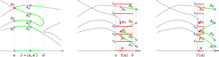
Figure 2.2: The left figure shows the generic case, where exactly one $x$-critical point ($p_{3}$) above $\alpha$ exists. The bottom-up method connects $A_{1}$ to $p_{1}$ and $A_{2}$ to $p_{2}$; the remaining arcs have to pass $p_{3}$. In the second figure, the fiber at $\alpha$ contains two critical points $p_{2}$ and $p_{3}.$ The red horizontal line segments pass through arbitrary chosen points $(\alpha,t_{i})$ separating $p_{i-1}$ and $p_{i}$. The initial isolating interval $I(\alpha)=(a,b)$ for $\alpha$ is not sufficient to determine the connections for all arcs since $A_{1},A_{2},A_{3}$ intersect the segments $I\times\{t_{i}\}.$ On the right, the refined isolating interval $I^{\prime}(\alpha)$ induces boxes $I^{\prime}(\alpha)\times(t_{i},t_{i+1})$ small enough such that no arc crosses the horizontal boundaries. By examination of the $y$-coordinates of the intersections between the arcs and the fiber over the right-hand boundary of $I^{\prime}(\alpha)$ (red crosses), we can match arcs and critical points.

In the second step of FastLift, we aim to isolate all (complex) roots of $f(\alpha,y)$. The above computation of an upper bound $m_{\alpha}^{*}$ motivates the following ansatz: In order to determine the roots of $f(\alpha,y)$, we combine a numerical complex solver for $f(\alpha,y)$ and an exact certification step. More precisely, we use the numerical solver to determine disjoint discs $D_{1},\ldots,D_{m}$ in the complex space and an exact certification step to certify the existence of a certain number $m_{i}\geq 1$ of roots (counted with multiplicity) of $f(\alpha,y)$ within each $D_{i}$; see Section 2.2 for details. Increasing the working precision and the number of iterations for the numerical solver eventually leads to arbitrary well refined discs $D_{i}$ – but without a guarantee that these discs are actually isolating! Since $m_{\alpha}^{*}$ constitutes an upper bound on the number of distinct complex roots of $f(\alpha,y)$, we must have $m\leq m_{\alpha}\leq m_{\alpha}^{*}$ at any time. Hence, if the number of discs $m$ equals the upper bound $m_{\alpha}^{*}$, we know for sure that all complex roots of $\deg f(\alpha,y)$ are isolated. Then, the isolating discs $D_{1},\ldots,D_{m}$ are further refined until, for all $i=1,\ldots,m$,

$$D_{i}\cap\mathbb{R}=\emptyset\text{ or }\bar{D}_{i}\cap D_{j}=\emptyset\text{ for all }j\neq i,$$ (2.6)

where $\bar{D}_{i}:=\{\bar{z}:z\in D_{i}\}$ denotes the complex conjugate of $D_{i}$. The latter condition guarantees that each disc $D_{i}$ which intersects the real axis actually isolates a real root of $f(\alpha,y)$. In addition, for each real root isolated by some $D_{i}$, we further obtain its multiplicity $m_{i}$ as a root of $f(\alpha,y)$.

If $m\neq m_{\alpha}^{*}$, either one of the roots of $f(\alpha,y)$ is still not isolated or it holds $m_{\alpha}<m_{\alpha}^{*}$. In the case that we do not succeed, that is, we still have $m<m_{\alpha}^{*}$ after a number of iterations (in the implementation, this number is set empirically) with increasing precision, we stop FastLift and proceed with Lift instead. In Section 2.3, we discuss the few failure cases.

We remark that the usage of Teissier’s formula is not entirely new when computing the topology of algebraic curves. In [12, 29], the formula (2.1) was used in its simplified form to compute $\operatorname*{mult}(\beta,f(\alpha,y))$ for a non-singular point $p=(\alpha,\beta)$ (i.e., $\operatorname*{Int}(f_{x},f_{y},p)=0$). In contrast, we use the formula in its general form and sum up the information along the entire fiber which eventually leads to the upper bound $m_{\alpha}^{*}$ on the number of distinct complex roots of $f(\alpha,y)$.

2.1.3 Connection Phase

Let us consider a fixed $x$-critical value $\alpha$, the corresponding isolating interval $I(\alpha)=(a,b)$ computed in the projection phase and the points $p_{i}:=(\alpha,y_{\alpha,i})\in C$, $i=1,\ldots,m_{\alpha}$, located on $C$ above $\alpha$. Furthermore, let $I=(\alpha,\alpha^{\prime})$ be the interval connecting $\alpha$ with the nearest $x$-critical value to the right of $\alpha$ (or $+\infty$ if none exists) and $A_{j}$, $j=1,\ldots,m_{I}$, the $j$-th arc of $C$ above $I$ with respect to vertical ordering. To its left, $A_{j}$ is either connected to $(\alpha,\pm\infty)$ (in case of a vertical asymptote) or to one of the points $p_{i}$. In order to determine the point to which an arc $A_{j}$ is connected, we consider the following two distinct cases:

• The generic case, in which there exists exactly one real $x$-critical point $p_{i_{0}}$ above $\alpha$ and $\deg f(\alpha,y)=\deg_{y}f$. The latter condition implies that $C$ has no vertical asymptote at $\alpha$. Then, the points $p_{1},\ldots,p_{i_{0}-1}$ must be connected with $A_{1},\ldots,A_{i_{0}-1}$ in button-up fashion, respectively, since, for each of these points, there exists a single arc of $C$ passing this point. The same argument shows that $p_{i_{0}+1},\ldots,p_{m_{\alpha}}$ must be connected to $A_{m_{I}-m_{\alpha}+i_{0}+1},\ldots,A_{m_{I}}$ in top-down fashion, respectively. Finally, the remaining arcs in between must all be connected to the $x$-critical point $p_{i_{0}}$.

• The non-generic case: Each arc $A_{j}$ is represented by a point $a_{j}:=(q_{I},y_{I,j})\in C$, where $y_{I,j}$ denotes the $j$-th real root of $f(q_{I},y)$ and $q_{I}$ an arbitrary but fixed rational value in $I$. We choose arbitrary rational values $t_{1},\ldots,t_{m_{\alpha}+1}$ with $t_{1}<y_{\alpha,1}<t_{2}<\ldots<y_{\alpha,m_{\alpha}}<t_{m_{\alpha}+1}$. Then, the points $\tilde{p}_{i}:=(\alpha,t_{i})$ separate the $p_{i}$’s from each other. Computing such $\tilde{p}_{i}$ is easy since we have isolating intervals with rational endpoints for each of the roots $y_{\alpha,i}$ of $f(\alpha,y)$. In a second step, we use interval arithmetic to obtain intervals $\mathfrak{B}f(I(\alpha)\times t_{i})$ with $f(I(\alpha)\times t_{i})\subset\mathfrak{B}f(I(\alpha)\times t_{i})$. As long as there exists an $i$ with $0\in\mathfrak{B}f(I(\alpha)\times t_{i})$, we refine $I(\alpha)$. Since none of the $\tilde{p}_{i}$ is located on $C$, we eventually obtain a sufficiently refined interval $I(\alpha)$ with $0\notin\mathfrak{B}f(I(\alpha)\times t_{i})$ for all $i$. It follows that none of the arcs $A_{j}$ intersects any line segment $I(\alpha)\times t_{i}$. Hence, above $I(\alpha)$, each $A_{j}$ stays within the the rectangle bounded by the two segments $I(\alpha)\times t_{i_{0}}$ and $I(\alpha)\times t_{i_{0}+1}$ and is thus connected to $p_{i_{0}}$. In order to determine $i_{0}$, we compute the $j$-th real root $\gamma_{j}$ of $f(b,y)\in\mathbb{Q}[y]$ and the largest $i_{0}$ such that $\gamma_{j}>t_{i_{0}}$. In the special case where $\gamma_{j}<t_{i}$ or $\gamma_{j}>t_{i}$ for all $i$, it follows that $A_{j}$ is connected to $(\alpha,-\infty)$ or $(\alpha,+\infty)$, respectively.

For the arcs located to the left of $\alpha$, we proceed in exactly the same manner. This concludes the connection phase and, thus, the description of our algorithm.

2.2 Numerical Solver with Certificate

In FastLift, we deploy a certified numerical solver for a fiber polynomial to find regions certified to contain its complex roots. Bini and Fiorentino presented a highly efficient solution to this problem in their MPSolve package [8]. We adapt their approach in a way suited to handle the case where the coefficients are not known a priori, but rather in an intermediate representation which can be refined to any arbitrary finite precision. The description given in this section is high-level. For the details of an efficient implementation, we refer the reader to [26]. In the following considerations, let $g(z):=f(\alpha,z)=\sum_{i=0}^{n}g_{i}z^{i}\in\mathbb{R}[z]$ be the fiber polynomial at an $x$-critical value $\alpha$ and $V(g)=\{\zeta_{i}\}$, $i=1,\dots,n,$ its complex roots. Thus, $g(z)=g_{n}\allowbreak\prod_{i=1}^{n}\allowbreak(z-\zeta_{i})$.

The main algorithm used in the numerical solver is the Aberth-Ehrlich iteration for simultaneous root finding. Starting from arbitrary distinct root guesses $(z_{i})_{i=1,\dots,n}$, it is given by the component-wise iteration rule $z^{\prime}_{i}=z_{i}$ if $g(z_{i})=0$, and

$$z^{\prime}_{i}=z_{i}-\frac{g(z_{i})/g^{\prime}(z_{i})}{1-g(z_{i})/g^{\prime}(z_{i})\cdot\sum_{j\neq i}\frac{1}{z_{i}-z_{j}}}$$

otherwise. As soon as the approximation vector $(z_{i})_{i}$ lies in a sufficiently small neighborhood of some permutation of the actual roots $(\zeta_{i})_{i}$ of $g$, this iteration converges with cubic order [34]. In practice, Aberth’s method shows excellent performance even if started from an arbitrary configuration far away from the solutions.

A straightforward implementation of [8] expects the coefficients $g_{i}$ of $g$ to be known up to some relative precision $p$, that is, the input is a polynomial $\tilde{g}=\sum\tilde{g_{i}}x^{i}$ whose floating point coefficients satisfy $\left|\tilde{g_{i}}-g_{i}\right|\leq 2^{-p}\left|g_{i}\right|$. In particular, this requirement implies that we have to decide in advance whether a coefficient vanishes. In general, though, the critical $x$-coordinate $\alpha$ of the fiber polynomial, and thus the coefficients of $g$, are not rational. Thus, it translates to expensive symbolic $\gcd$ computations of $R$ and the coefficients of $f$ as a univariate polynomial in $\mathbb{Z}[y][x]$.

Instead, we work on a Bitstream interval representation [16, 26] $[g]^{\mu}$ of $g$. Its coefficients are interval approximations of the coefficients of $g$, where we require the width $|g_{i}^{+}-g_{i}^{-}|$ of each coefficient $[g]^{\mu}_{i}=[g_{i}^{-},g_{i}^{+}]$ to be $\leq\mu$ for a certain absolute precision $\mu=2^{-p}$. In this sense $[g]^{\mu}$ represents the set $\{\tilde{g}:\tilde{g_{i}}\in[g]^{\mu}_{i}\}$ of polynomials in a $\mu$-polynomial neighborhood of $g$; in particular, $g$ itself is contained in $[g]^{\mu}$. Naturally, for the interval boundaries, we consider dyadic floating point numbers (bigfloats). Note that we can easily compute arbitrarily good Bitstream representations of $f(\alpha,z)$ by approximating $\alpha$ to an arbitrary small error, for example using the quadratic interval refinement technique [1].

Starting with some precision (say, $\mu=2^{-53}$) and a vector of initial approximations, we perform Aberth’s iteration on some representant $\tilde{g}\in[g]^{\mu}$. The natural choice is the median polynomial with $\tilde{g_{i}}=(g_{i}^{-}+g_{i}^{+})/2$, but we take the liberty to select other candidates in case of numerical singularities in Aberth’s rule (most notably, if $\tilde{g}^{\prime}(z_{i})=0$ in some iteration).

After a finite number of iterations (depending on the degree of $g$), we interrupt the iteration and check whether the current approximation state already captures the structure of $V(g)$. We use the following result by Neumaier and Rump [31], founded in the conceptually similar Weierstraß-Durand-Kerner simultaneous root iteration:

Lemma 2 (Neumaier)

Let $g(z)=g_{n}\prod_{i=1}^{n}(z-\zeta_{i})\in\mathbb{C}[z]$, $g_{n}\neq 0$. Let $z_{i}\in\mathbb{C}$ for $i=1,\dots,n$ be pairwise distinct root approximations. Then, all roots of $g$ belong to the union $\mathcal{D}$ of the discs

$$D_{i}:=D(z_{i}-r_{i},|r_{i}|),$$

$$\text{where }r_{i}:=\frac{n}{2}\cdot\frac{\omega_{i}}{g_{n}}\text{ and }\omega_{i}:=\frac{g(z_{i})}{\prod\nolimits_{j\neq i}(z_{i}-z_{j})}.$$

Moreover, every connected component $C$ of $\mathcal{D}$ consisting of $m$ discs contains exactly $m$ zeros of $g$, counted with multiplicity.

The above lemma applied to $[g]^{\mu}$ using conservative interval arithmetic yields a superset $\mathcal{C}=\{C_{1},\dots,C_{m}\}$ of regions and corresponding multiplicities $\lambda_{1},\dots,\lambda_{m}$ such that, for each $C_{k}\in\mathcal{C}$, all polynomials $\tilde{g}\in[g]^{\mu}$ (and, in particular, $g$) have exactly $\lambda_{k}$ roots in $C_{k}$ counted with multiplicities. Furthermore, once the quality of the approximations $(z_{i})_{i}$ and $[g]^{\mu}$ is sufficiently high, $\mathcal{C}$ converges to $V(g)$.

In FastLift, where we aim to isolate the roots of $g:=f(\alpha,y)$, we check whether $m=m_{\alpha}^{*}$. If the latter equality holds, Teissier’s lemma guarantees that the regions $C_{k}\in\mathcal{C}$ are isolating for the roots of $g$, and we stop. Otherwise, we repeat Aberth’s iteration after checking whether $0\in[g]^{\mu}(z_{i})$. Informally, if this holds the quality of the root guess is not distinguishable from any (possibly better) guess within the current interval approximation of $g$, and we double the precision ($\mu^{\prime}=\mu^{2}$) for the next stage.

Aberth’s iteration lacks a proof for convergence in the general case and, thus, cannot be considered complete. However, we feel this is a merely theoretical issue: to the best of our knowledge, only artificially constructed, highly degenerate configurations of initial approximations render the algorithm to fail. Regardless of this assumption, the regions $C_{k}\in\mathcal{C}$ are certified to comprise the roots of $g$ at any stage of the algorithm by Neumaier’s lemma and the rigorous use of interval arithmetic. Furthermore, since we use the numerical method as a filter only, the completeness of the overall approach is not harmed.

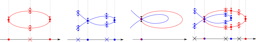
Figure 2.3: The two figures on the left show the topology analyses for the curves $C=V(f)$ and $D=V(g)$. The figure in the middle shows the intersection of the two curves. For the curve pair analysis, critical event lines (at dots) are sorted and non-critical event lines (at crosses) in between are inserted. Finally, for each event line $x=\alpha$, the roots of $f(\alpha,y)$ and $g(\alpha,y)$ are sorted. The latter task is done by further refining corresponding isolating intervals (blue or red intervals) and using the combinatorial information from the curve analyses and the computation of the intersection points.

2.3 Discussion

We conclude our description of the curve analysis algorithm with the following discussion on our method FastLift in the lifting step. FastLift is a certified method, that is, in case of success, it returns the mathematical correct result. However, the reader may notice that FastLift does not apply in all cases, a reason why we additionally consider the complete but less efficient backup method Lift for some of the $x$-critical fibers. The failure of FastLift is either due to a very special geometric situation along a certain fiber or due to the behavior of the numerical solver. Special geometric situations are:

1. $C$ has a vertical tangent at $x=\alpha$ and $f(\alpha,y)$ is not square-free, or

2. there exists an intersection point of $f_{x}^{*}=\frac{f_{x}}{\gcd(f_{x},f_{y})}$ and $f_{y}^{*}=\frac{f_{y}}{\gcd(f_{x},f_{y})}$ above an $x$-critical value $\alpha$ of $f$ which is not located on $C$.

In case that none of the above special geometric situations is given (or removed by applying a shear; see below), the success of FastLift is guaranteed if the following conditions on the numerical solver are fulfilled:

1. The numerical solver is run for sufficiently many iterations, and

2. the approximations returned by the numerical solver converge against the roots of $f(\alpha,y)$ when increasing precision and number of iterations.

As already mentioned in Section 2.2, we consider (Num2) as an exclusively theoretical problem. We further remark that, alternatively, we can use an exact and complete complex bitstream solver [32] to compute arbitrary good approximations of the fiber polynomial $f(\alpha,y)$, an approach which can be considered as an extension of Bdc to complex roots. However, for efficiency reasons, we decided to integrate a numerical method into our implementation instead. (Num1) is a practical problem and, in our implementation, we just empirically set the maximal number of iterations and the maximal precision as parameters depending on the degree and the bitsize of the polynomials. We noticed that the success of FastLift actually depends on these parameter values and consider it an interesting research question how they should be related to the given input to achieve optimal running times.

It is worth mentioning that a complete and exact topology computation can be fully based on FastLift if we allow shearing (i.e., a coordinate transformation $x\mapsto x+sy$ for a $s\in\mathbb{Q}$). Namely, for all but except a finite number $N$ of shearing factors, (Geo1) and (Geo2) do not apply to the sheared curve. Hence, when considering $N+1$ pairwise distinct shearing factors one by one in circular order and increasing the number of iterations and the precision in the numerical solver for each factor, FastLift eventually succeeds for all fibers.

In practice, as observed in our experiments presented in Section 4, the failure conditions for FastLift are almost negligible, as the method only fails for a few critical fibers on very special instances. For the remaining fibers and for all fibers of the majority of instances, FastLift is successful and extremely fast.

3 Arrangement Computation

Cgal’s recent implementation for computing arrangements of planar algebraic curves reduces all required geometric constructions (as intersections) and predicates (as comparisons of points and $x$-monotone curves) to the geometric-topological analysis of a single curve [18] and pairs of curves [17]; see also [5] and Cgal’s documentation [36].

Beyond the improved curve analysis proposed in Section 2, we aim to avoid subresultant sequences in general when analysing pairs of curves (see illustration in Figure 2.3), which is straightforward given the analyses of each single curve and the common intersection points of the two curves computed by Bisolve:

Let $C=V(f)$ and $D=V(g)$ be two planar algebraic curves implicitly defined by the square-free polynomials $f$, $g\in\mathbb{Z}[x,y]$. The curve analysis for $C$ provides a set of critical event lines $x=\alpha$, where $f(\alpha,y)$ is non square-free. Each $\alpha$ is represented as the root of a square-free polynomial $r_{i}$, with $r_{i}$ a factor of $R_{C}:=\operatorname{(}f,f_{y},y)$, together with an isolating interval $I(\alpha)$. In addition, we have isolating intervals for the roots of $f(\alpha,y)$. A corresponding result also holds for the curve $D$ with $R_{D}:=\operatorname*{res}(g,g_{y},y)$. For the common intersection points of $C$ and $D$, a similar representation is known. That is, we have critical event lines $x=\alpha^{\prime}$, where $\alpha^{\prime}$ is a root of a square-free factor of $R_{CD}:=\operatorname{res}(f,g,y)$ and, thus, $f(\alpha,y)$ and $g(\alpha,y)$ share at least one common root (or the their leading coefficients both vanish for $x=\alpha$). In addition, isolating intervals for each of these roots are computed. The curve-pair analysis now essentially follows from merging this information. More precisely, we first compute merged critical event lines (via sorting the roots of $R_{C}$, $R_{D}$ and $R_{CD}$) and, then, pad merged non-critical event lines at rational values $q_{I}$ in between. The intersections of $C$ and $D$ with a non-critical event line at $x=q_{I}$ are easily computed by isolating the roots of $f(q_{I},y)$ and $g(q_{I},y)$ and further refining the isolating intervals until all isolating intervals are pairwise disjoint. For a critical event line $x=\alpha$, we refine the already computed isolating intervals for $f(\alpha,y)$ and $g(\alpha,y)$ until the number of pairs of overlapping intervals matches the number $m$ of intersection points of $C$ and $D$ above $\alpha$. This number is obtained from the output of Bisolve applied to $f$ and $g$, restricted to $x=\alpha$. The information on how to connect the lifted points is provided by the curve analyses for $C$ and $D$.

We remark that, in the previous approach by Eigenwillig and Kerber [17], $m$ is determined via efficient filter methods, too, while in general, a subresultant computation is needed if the filters fail. This is, for instance, the case when two covertical intersections of $C$ and $D$ occur.

4 Implementation and Experiments

Setup. We have implemented our algorithms as a branch of the bivariate algebraic kernel released with version 3.7 in October 2010, and replaced the curve and curve-pair analyses therein with our new methods based on FastLift, Lift and Bisolve. As throughout Cgal, we follow the generic programming paradigm, which allows us to choose among various number types and methods to isolated the real roots of integral univariate polynomials. For our setup, we rely on the number types provided by Gmp 5.0.1 and the highly efficient univariate solver based on the Descartes method contained in Rs by Fabrice Rouillier [30], which is also the basis for Isolate in Maple 13.

All experiments have been conducted on 2.8 GHz $8$-Core Intel Xeon W3530 with 8 MB of L2 cache on a Linux platform. For the GPU-part of the algorithm, we have used the GeForce GTX580 graphics card (Fermi Core). All used data sets are available for download.

Symbolic Speedups. Our algorithm exclusively relies on two symbolic operations, that is, resultant and $\gcd$ computation. We outsource both computations to the graphics hardware to reduce the overhead of symbolic arithmetic which typically constitutes the main bottleneck in previous approaches. Besides a quick introduction given next, we refer the interested reader to [20, 21, 22] for more details.

Shortly, both approaches are based on the “divide-conquer-combine” principle used in the modular algorithms by Brown [10] and Collins [14]. This principle allows to distribute the computation over a large number of processor cores of the graphics card. At highest level, the modular approach can be formulated as follows. 1. Apply modular and/or evaluation homomorphisms to reduce the problem to a large set of subproblems over a simple domain. 2. Solve the subproblems individually in a finite field. 3. Recover the result with polynomial interpolation (in case evaluation homomorphism has been applied) and Chinese remaindering.

Altogether, the GPU realization is quite straightforward and does not deserve much attention within the context of this work. It is only worth noting that our implementation of univariate $\gcd$s on the graphics card is comparable in speed with the one from Ntl 5.5 running on the host machine. Our intuition for this is because, in contrast to bivariate resultants, computing a $\gcd$ of moderate degree univariate polynomials does not provide a sufficient amount of parallelism, and Ntl’s implementation is nearly optimal. Moreover, the time for initial modular reduction of polynomials, still performed on the CPU, can become noticeably large, thereby neglecting the efficiency of the GPU algorithm. Yet, we find it very promising to perform the modular reduction on the GPU which should further speed-up our algorithm.

Contestants. We compare the new implementation with Cgal’s bivariate algebraic kernel (see [5] and [6]) that has shown excellent performance in exhaustive experiments over existing approaches, namely cad2d and Isotop [23] which is based on Rs. Both contestants were, except for few example instances, less efficient than Cgal’s implementation, so that we omit further tests with them. Two further reasons can be given: Firstly, we enhanced Cgal’s kernel with GPU-supported resultants and $\gcd$s, which makes it more competitive to existing software, but also to our new software, in case of non-singular curves, though slowdowns are still expected for singular curves or curves in non-generic position due to the need of subresultants sequences performed on the CPU. Secondly, the contestants based on Rs require as subtask Rs to solve the bivariate polynomial system $f=f_{y}=0$ in the curve-analysis. In [4], we learned that the GPU-supported Bisolve was at least competitive to the current version of Rs and even showed in most cases an excellent speed gain over Rs. However, Rs is currently getting a very budding polish based on Rational Univariate Representations and modular arithmetic. Its theory will be presented at EuroCG 2011 [9]. We are looking forward to compare our algorithms with a preliminary version of the new Rs quite soon. Moreover, we are confident that the authors will support the computation of arrangements of algebraic curves in a similar setup. Though tackling the same problem, both realizations can be seen as orthogonal if not complementary.

4.1 Curve Analysis

We first present the experiments comparing the analyses of single algebraic curves for different families of curves: (R) random curves of various degree and bit-lengths of their coefficients, (I) curves interpolated through points on a grid, (S) curves in the two-dimensional parameter space of a sphere, (T) curves that were constructed by multiplying a curve $f(x,y)$ with $f(x,y+1)$, such that each fiber has more than one critical point. (P) projections of intersections of algebraic surfaces in 3D and, finally, (X) “special” curves of degrees up to 42 with many singularities or high-curvature points. We already considered these special curves in [4] and describe them in more detail in Table 5 in Appendix A. The non-random and non-special curves are taken from [25, 4.3]. For the curve topology analysis, we consider four different setups: (a) Bisolveis, strictly speaking, not comparable with the actual curve analysis as it only computes the solutions of the system $f=f_{y}=0$. Still, it is interesting to see that our new hybrid method even outperforms this algorithm that only solves a subproblem of the curve-analysis. (b) LiftAnaexclusively uses Lift for the fiber computations. (c) FastAnacombines FastLift and Lift in the fiber computations. More precisely, it uses FastLift first, and if it fails for a certain fiber, Lift is considered for this fiber instead, (d) Ak_2is the bivariate algebraic kernel shipped with Cgal 3.7, but with GPU-supported resultants and $\gcd$s. FastAna is our default setting, and its running time also includes the timing for the fiber computations where FastLift fails and Lift is applied instead.

Table 1: Running times (in sec) for analyses of algebraic curves of various families; timeout: algorithm timed out ($>$ 400 sec)

(R) sets of five random curves
degree, bits	Bisolve	LiftAna	FastAna	Ak_2
dense curves
9, 0010	0.83	0.73	0.24	0.66
9, 2048	4.17	9.00	2.24	3.43
15, 0010	2.82	3.47	1.01	2.21
15, 2048	20.48	50.06	13.31	16.82
sparse curves
9, 0010	0.25	0.33	0.11	1.00
9, 2048	0.25	0.39	0.15	0.98
15, 0010	1.50	3.31	0.57	3.19
15, 2048	15.66	32.15	8.08	24.32
(I) curve interpolated through points on a grid
degree	Bisolve	LiftAna	FastAna	Ak_2
9	4.51	7.25	2.50	4.98
12	25.25	45.58	14.66	27.07
(S) parametrized curve on a sphere with 16bit-coefficients
degree	Bisolve	LiftAna	FastAna	Ak_2
6	6.52	8.17	2.49	14.65
9	51.92	78.09	24.14	45.66
(T) curves wih a vertically translated copy
degree	Bisolve	LiftAna	FastAna	Ak_2
6	5.27	3.15	0.83	12.89
9	14.78	14.91	2.97	159.22
(P) projected intersection curve of surfaces with 8bit-coefficient
degree(s)	Bisolve	LiftAna	FastAna	Ak_2
$2\cdot 2$	0.26	0.23	0.09	0.22
$3\cdot 3$	2.87	1.75	0.52	1.97
$4\cdot 4$	10.01	11.93	2.24	38.91
$5\cdot 5$	83.00	95.37	13.76	timeout
(X) special curves (see Table 5, Appendix B for descriptions)
name	Bisolve	LiftAna	FastAna	Ak_2
curve_issac	2.89	2.30	0.44	2.96
SA_2_4_eps	0.35	2.18	0.64	73.00
grid_deg_10	1.32	2.52	0.79	1.54
L6_circles	4.52	92.24	2.10	224.19
huge_cusp	8.50	18.40	5.50	16.10
swinnerton	19.61	16.81	7.12	304.09
degree_7_surf	14.57	48.94	7.39	timeout
spider	57.09	195.21	26.26	timeout
FTT_5_4_4	11.70	44.27	32.23	timeout
challenge_12b	16.48	52.71	44.30	timeout
mignotte_xy	260.61	270.70	136.54	timeout

Table 1 lists the running times for single-curve analyses. We only give the results for representative examples; complete tables are given in Appendix A. It is easy to see that FastLift is generally superior to the existing kernel, even though Cgal’s implementation profits from GPU-accelerated symbolic arithmetic. Moreover, while the speed-up for curves in generic position is already considerable (about half of the time), it becomes even more impressive for projected intersection curves of surfaces and “special” curves with singularities. The reason for this tremendous speed-up is that, for singular curves, Ak_2’s performance drops significantly with the degree of the curve when the time to compute subresultants on the CPU becomes the dominating bottleneck of that approach. In addition, for curves in non-generic position, the efficiency of Ak_2 is affected because a coordinate transformation has to be considered in these cases.

Recall that the symbolic-numerical filter in FastLift fails for very few instances, in which case Lift is locally used instead. The switch to the backup method is observable in timings; see for instance, challenge_12b. As a result, the difference of the running times between Lift and FastLift are considerably less than for instances where the filter method succeeds for all fibers. In these cases, the numerical solver cannot isolate the roots within a given number of iterations, or we indeed have $m<m^{*}_{\alpha}$; see Section 2.3. Nevertheless, the running times are still very promising and yet perform better than Ak_2 for non-generic input, even though Lift’s implementation is not yet mature enough, and we anticipate a further performance improvement.

Similar as Ak_2 has improved on previous approaches when it was presented in 2008, our new methods improve on Ak_2 now. That is, for random, interpolated and parametrized curves, the speed gain is noticeable, while for translated curves and projected intersections, we improve the more the higher the degrees. On special curves of large degree(!), we improve by a factors up to 100 and more.

4.2 Arrangements

For arrangements of algebraic curves, we compare two implementations: (A) Ak_2is Cgal’s bivariate algebraic kernel shipped with Cgal 3.7 but with GPU-supported resultants and gcds. (B) FastKernelis the same, but relies on FastLift-filtered analyses of single algebraic curves. For the curve pair analysis, FastKernel exploits Ak_2’s functionality whenever subresultant computations are not needed (i.e., a unique transversal intersection of two curves along a critical event line). For more difficult situations (i.e., two covertical intersections or a tangential intersection), the curve pair analysis uses Bisolve as explained in Section 3. Our testbed consists of sets of curves from different families: (F) random rational functions of various degree (C) random circles (E) random ellipses (R) random curves of various degree and coefficient bit-length (P) sets of projected intersection curves of algebraic surfaces , and, finally, (X) combinations of “special” curves.

Table 2: Running times (in sec) for computing arrangements of algebraic curves; timeout: algorithm timed out ($>$ 4000 sec)

(P) increasing number of projected surface intersections
#resultants	FastKernel	Ak_2
2	0.21	0.49
3	0.48	0.93
4	1.03	1.64
5	2.44	3.92
6	5.14	7.84
7	13.65	21.70
8	22.69	35.77
9	41.53	67.00
10	58.37	91.84
(X) combinations of special curves (see Table 5, Appendix B)
#curves	FastKernel	Ak_2
2	9.2	81.93
3	25.18	148.46
4	248.87	730.57
5	323.42	836.43
6	689.39	3030.27
7	757.94	3313.27
8	1129.98	timeout
9	1166.17	timeout
10	1201.34	timeout
11	2696.15	timeout

We skip the tables for rational functions, circles, ellipses and random curves because the performance of both contestants are more or less equal: The linearly many curve-analyses are simple and, for the quadratic number of curve-pair analyses, there are typically no multiple intersections along a fiber, that is, Bisolve is not triggered. Thus, the execution paths of both implementations are almost identical, but only as we enhanced Ak_2 with GPU-enabled resultants and $\gcd$s. In addition, we also do not expect the need of a shear for such curves, thus, the behavior is anticipated. The picture changes for projected intersection curves of surfaces and combinations of special curves whose running times are reported in Table 2. The Ak_2 requires for both sets expensive subresultants to analyze single curves and to compute covertical intersections, while FastKernel’s performance is crucially less affected in such situations.

Appendix A Further Experiments of Curve Analyses

Table 3: Running times (in sec) for analyses of random algebraic curves; timeout: algorithm timed out ($>$ 400 sec)

(R) sets of five random curves
degree, bits	Bisolve	LiftAna	FastAna	Ak_2
dense curves
6, 0010	0.38	0.39	0.15	0.36
6, 0128	0.32	0.49	0.18	0.32
6, 0512	0.55	0.89	0.35	0.55
6, 2048	1.85	3.50	0.99	1.71
9, 0010	0.83	0.73	0.24	0.66
9, 0128	0.57	0.90	0.31	0.55
9, 0512	1.04	1.91	0.57	0.96
9, 2048	4.17	9.00	2.24	3.43
12, 0010	2.18	2.21	0.69	1.77
12, 0128	1.64	2.87	0.86	1.46
12, 0512	2.84	6.09	1.56	2.55
12, 2048	12.07	30.26	7.06	9.96
15, 0010	2.82	3.47	1.01	2.21
15, 0128	2.36	4.55	1.29	2.06
15, 0512	4.40	9.84	2.63	3.77
15, 2048	20.48	50.06	13.31	16.82
sparse curves
6, 0010	0.17	0.21	0.12	0.22
6, 0128	0.14	0.19	0.09	0.22
6, 0512	0.21	0.36	0.12	0.39
6, 2048	0.73	1.13	0.39	1.06
9, 0010	0.25	0.33	0.11	1.00
9, 0128	0.25	0.39	0.15	0.98
9, 0512	0.43	0.65	0.23	1.43
9, 2048	1.53	2.51	0.85	4.31
12, 0010	0.41	0.83	0.19	1.67
12, 0128	0.40	1.05	0.25	1.60
12, 0512	0.78	2.16	0.50	2.53
12, 2048	3.82	10.54	2.82	9.94
15, 0010	1.50	3.31	0.57	3.19
15, 0128	1.48	3.98	0.72	2.99
15, 0512	2.96	7.10	1.45	5.58
15, 2048	15.66	32.15	8.08	24.32

Table 4: Running times (in sec) for analyses of algebraic curves of various families; timeout: algorithm timed out ($>$ 400 sec)

(I) curve interpolated through points on a grid
degree	Bisolve	LiftAna	FastAna	Ak_2
5	0.41	0.50	0.21	0.49
6	0.72	1.13	0.41	0.84
7	1.42	2.20	0.78	1.62
8	2.59	3.78	1.32	2.86
9	4.51	7.25	2.50	4.98
10	6.62	11.52	3.62	7.65
11	12.38	23.27	7.25	13.93
12	25.25	45.58	14.66	27.07
13	48.97	93.97	27.90	46.21
14	101.96	193.61	59.14	90.27
15	211.95	timeout	114.68	166.68
16	timeout	timeout	236.39	314.61
(S) parametrized curve on a sphere with 16bit-coefficients
degree	Bisolve	LiftAna	FastAna	Ak_2
6	6.52	8.17	2.49	14.65
7	22.58	27.39	8.47	16.83
8	37.94	53.3	16.25	32.09
9	51.92	78.09	24.14	45.66
10	72.21	110.81	32.38	64.31
(T) curves with a vertically translated copy
degree	Bisolve	LiftAna	FastAna	Ak_2
5	3.95	1.93	0.6	5.61
6	5.27	3.15	0.83	12.89
7	7.31	6.14	1.28	33.97
8	9.66	7.99	1.75	73.59
9	14.78	14.91	2.97	159.22
10	17.03	15.78	3.36	timeout
(P) projected intersection curve of surfaces with 8bit-coefficient
degree(s)	Bisolve	LiftAna	FastAna	Ak_2
$2\cdot 2$	0.26	0.23	0.09	0.22
$2\cdot 3$	0.39	0.40	0.12	0.32
$2\cdot 4$	1.03	0.77	0.25	0.73
$2\cdot 5$	1.97	1.53	0.44	1.93
$3\cdot 3$	2.87	1.75	0.52	1.97
$3\cdot 4$	3.63	3.02	0.67	5.21
$3\cdot 5$	8.71	9.22	1.90	25.87
$4\cdot 4$	10.01	11.93	2.24	38.91
$4\cdot 5$	21.45	28.22	4.46	231.64
$5\cdot 5$	83.00	95.37	13.76	timout
(X) special curves (see Table 5, Appendix B for desciptions)
name	Bisolve	LiftAna	FastAna	Ak_2
curve_issac	2.89	2.30	0.44	2.96
L4_circles	1.56	8.80	0.52	9.92
SA_2_4_eps	0.35	2.18	0.64	73.00
grid_deg_10	1.32	2.52	0.79	1.54
ten_circles	6.77	3.79	0.82	24.07
dfold_10_6	4.45	4.62	1.58	30.80
L6_circles	4.52	92.24	2.10	224.19
cov_sol_20	8.68	12.16	3.38	65.05
curve24	14.07	15.61	4.07	50.73
huge_cusp	8.50	18.40	5.50	16.10
swinnerton	19.61	16.81	7.12	304.09
degree_7_surf	14.57	48.94	7.39	timeout
challenge_12a	7.47	15.84	14.41	timeout
spider	57.09	195.21	26.26	timeout
FTT_5_4_4	11.70	44.27	32.23	timeout
challenge_12b	16.48	52.71	44.30	timeout
mignotte_xy	260.61	270.70	136.54	timeout

Appendix B Description of Special Curves

Table 5: Description of the special curves used in the experiments of Section 4. Sources of curves are given where known.

Instance	$y$-degree	Description
curve_issac	15	isolated points, high-curvature points [13]
L4_circles	16	4 circles w.r.t. L4-norm; clustered solutions
SA_2_4_eps	16	singular points with high tangencies, displaced [27]
grid_deg_10	10	large coefficients; curve in generic position
ten_circles	20	set of 10 random circles multiplied together; rational solutions
dfold_10_6	30	many half-branches [27]
L6_circles	32	4 circles w.r.t. L6-norm; clustered solutions
cov_sol_20	20	covertical solutions
curve24	24	curvature of degree 8 curve; many singularities
huge_cusp	8	large coefficients; high-curvature points
swinnerton	25	covertical solutions in $x$ and $y$
degree_7_surf	42	silhouette of an algebraic surface; covertical solutions in $x$ and $y$
challenge_12a	30	many candidate solutions to be checked [27]
spider	12	degenerate curve; many clustered solutions
FTT_5_4_4	40	many non-rational singularities [27]
challenge_12b	40	many candidates to check [27]
mignotte_xy	42	a product of $x$/$y$-Mignotte polynomials, displaced; many clustered solutions

References

- [1] J. Abbott. Quadratic interval refinement for real roots, 2006. www.dima.unige.it/~abbott/publications/RefineInterval.pdf.
- [2] L. Alberti, B. Mourrain, and J. Wintz. Topology and Arrangement Computation of Semi-Algebraic Planar Curves. CAGD, 25(8):631–651, 2008.
- [3] S. Basu, R. Pollack, and M.-F. Roy. Algorithms in Real Algebraic Geometry, volume 10 of Algorithms and Computation in Mathematics. Springer, 2006.
- [4] E. Berberich, P. Emeliyanenko, and M. Sagraloff. An elimination method for solving bivariate polynomial systems: Eliminating the usual drawbacks. In ALENEX ’11, pages 35–47, San Francisco, USA, January 2011. Society for Industrial and Applied Mathematics (SIAM).
- [5] E. Berberich, M. Hemmer, and M. Kerber. A generic algebraic kernel for non-linear geometric applications. In SoCG ’11, Paris, France, June 2011. To appear.
- [6] E. Berberich, M. Hemmer, S. Lazard, L. Peñaranda, and M. Teillaud. Algebraic kernel. In CGAL User and Reference Manual 3.7. CGAL Editorial Board, 2010.
- [7] E. Berberich, M. Kerber, and M. Sagraloff. An efficient algorithm for the stratification and triangulation of algebraic surfaces. CGTA, 43:257–278, 2010. Special issue on SoCG ’08.
- [8] D. A. Bini and G. Fiorentino. Design, analysis, and implementation of a multiprecision polynomial rootfinder. Numerical Algorithms, 23:127–173, 2000.
- [9] Y. Bouzidi, S. Lazard, M. Pouget, and F. Rouillier. New bivariate system solver and topology of algebraic curves. In EuroCG ’11, Nancy, France, March 2011.
- [10] W. S. Brown. On Euclid’s algorithm and the computation of polynomial greatest common divisors. In SYMSAC ’71, pages 195–211, New York, NY, USA, 1971. ACM.
- [11] M. Burr, S. W. Choi, B. Galehouse, and C. K. Yap. Complete subdivision algorithms, II: Isotopic Meshing of Singular Algebraic Curves. In ISSAC ’08, pages 87–94. ACM, 2008.
- [12] J. Cheng, S. Lazard, L. Peñaranda, M. Pouget, F. Rouillier, and E. Tsigaridas. On the topology of real algebraic plane curves. MCS (special issue on Comp. Geom. and CAGD), 4(1):113–137, 2010.
- [13] J.-S. Cheng, X.-S. Gao, and J. Li. Root isolation for bivariate polynomial systems with local generic position method. In ISSAC ’09, pages 103–110, New York, NY, USA, 2009. ACM.
- [14] G. E. Collins. The calculation of multivariate polynomial resultants. In SYMSAC ’71, pages 212–222. ACM, 1971.
- [15] G. E. Collins and A. G. Akritas. Polynomial real root isolation using Descarte’s rule of signs. In SYMSAC ’76, pages 272–275, New York, NY, USA, 1976. ACM.
- [16] A. Eigenwillig. Real Root Isolation for Exact and Approximate Polynomials Using Descartes’ Rule of Signs. PhD thesis, Universität des Saarlandes, Saarbrücken, Germany, 2008.
- [17] A. Eigenwillig and M. Kerber. Exact and Efficient 2D-Arrangements of Arbitrary Algebraic Curves. In SoDA ’08, pages 122–131. ACM & SIAM, 2008.
- [18] A. Eigenwillig, M. Kerber, and N. Wolpert. Fast and Exact Geometric Analysis of Real Algebraic Plane Curves. In ISSAC ’07, pages 151–158. ACM, 2007.
- [19] A. Eigenwillig, L. Kettner, W. Krandick, K. Mehlhorn, S. Schmitt, and N. Wolpert. A Descartes algorithm for polynomials with bit-stream coefficients. In CASC ’05, volume 3718 of LNCS, pages 138–149, 2005.
- [20] P. Emeliyanenko. High-performance polynomial GCD computations on graphics processors. Submitted to HPCS ’11.
- [21] P. Emeliyanenko. A complete modular resultant algorithm targeted for realization on graphics hardware. In PASCO ’10, pages 35–43, New York, NY, USA, 2010. ACM.
- [22] P. Emeliyanenko. Modular Resultant Algorithm for Graphics Processors. In ICA3PP ’10, pages 427–440, Berlin, Heidelberg, 2010. Springer-Verlag.
- [23] L. Gonzalez-Vega and I. Necula. Efficient Topology Determination of Implicitly Defined Algebraic Plane Curves. CAGD ’02, 19(9):719–743, 2002.
- [24] J. Gwozdziewicz, A. Ploski, and J. G. Zdziewicz. Formulae for the singularities at infinity of plane algebraic curves, 2000.
- [25] M. Kerber. Geometric Algorithms for Algebraic Curves and Surfaces. PhD thesis, Saarland University, Saarbrücken, Germany, 2009.
- [26] A. Kobel. Certified Numerical Root Finding. Master’s thesis, Universität des Saarlandes, Saarbrücken, Germany, 2011.
- [27] O. Labs. A list of challenges for real algebraic plane curve visualization software. In Nonlinear Computational Geometry, volume 151 of The IMA Volumes, pages 137–164. Springer New York, 2010.
- [28] B. Mourrain and J.-P. Pavone. Subdivision methods for solving polynomial equations. Technical report, INRIA, Sophia Antipolis, France, 2005.
- [29] L. Peñaranda. Non-linear computational geometry for planar algebraic curves. PhD thesis, Uni. Nancy, 2010.
- [30] F. Rouillier and P. Zimmermann. Efficient isolation of polynomial’s real roots. J. Comput. Appl. Math., 162(1):33–50, 2004.
- [31] S. M. Rump. Ten methods to bound multiple roots of polynomials. J. Comp. Appl. Math., 156:403–432, 2003.
- [32] M. Sagraloff. A general approach to isolating roots of a bitstream polynomial. Mathematics in Computer Science, 2011. Accepted for publication, see also http://www.mpi-inf.mpg.de/~msagralo/bit11.pdf.
- [33] B. Teissier. Cycles évanescents, sections planes et conditions de whitney. (french). Singularités à Cargèse, (78):285–362, 1973.
- [34] P. Tilli. Convergence conditions of some methods for the simultaneous computation of polynomial zeros. Calcolo, 35:3–15, 1998.
- [35] J. von zur Gathen and J. Gerhard. Modern Computer Algebra. Cambridge University Press, New York, NY, USA, 2003.
- [36] R. Wein, E. Fogel, B. Zukerman, and D. Halperin. 2D arrangements. In CGAL User and Reference Manual 3.7. CGAL Editorial Board, 2010. http://www.cgal.org/Manual/3.7/doc_html/cgal_manual/packages.html#Pkg:A%rrangement2.