On the role of the magnetic dipolar interaction in cold and ultracold collisions: Numerical and analytical results for NH(${}^{3}\Sigma^{-}$) + NH(${}^{3}\Sigma^{-}$)

Abstract

We present a detailed analysis of the role of the magnetic dipole-dipole interaction in cold and ultracold collisions. We focus on collisions between magnetically trapped NH molecules, but the theory is general for any two paramagnetic species for which the electronic spin and its space-fixed projection are (approximately) good quantum numbers. It is shown that dipolar spin relaxation is directly associated with magnetic-dipole induced avoided crossings that occur between different adiabatic potential curves. For a given collision energy and magnetic field strength, the cross-section contributions from different scattering channels depend strongly on whether or not the corresponding avoided crossings are energetically accessible. We find that the crossings become lower in energy as the magnetic field decreases, so that higher partial-wave scattering becomes increasingly important below a certain magnetic field strength. In addition, we derive analytical cross-section expressions for dipolar spin relaxation based on the Born approximation and distorted-wave Born approximation. The validity regions of these analytical expressions are determined by comparison with the NH + NH cross sections obtained from full coupled-channel calculations. We find that the Born approximation is accurate over a wide range of energies and field strengths, but breaks down at high energies and high magnetic fields. The analytical distorted-wave Born approximation gives more accurate results in the case of $s$-wave scattering, but shows some significant discrepancies for the higher partial-wave channels. We thus conclude that the Born approximation gives generally more meaningful results than the distorted-wave Born approximation at the collision energies and fields considered in this work.

I Introduction

The ability to produce and trap atomic and molecular species at sub-kelvin temperatures offers numerous exciting possibilities in condensed-matter physics Greiner et al. (2002); Jaksch and Zoller (2005); Micheli et al. (2006); Bloch et al. (2008), quantum computing DeMille (2002); Gulde et al. (2003); André et al. (2006), high-precision spectroscopy Lev et al. (2006); Fortier et al. (2007); Bethlem and Ubachs (2009); Tarbutt et al. (2009); Poli et al. (2011), and physical chemistry van de Meerakker et al. (2005); Gilijamse et al. (2006, 2007); Campbell et al. (2007, 2008); Sawyer et al. (2008); Krems (2008); Campbell et al. (2009); Scharfenberg et al. (2010); Ospelkaus et al. (2010). Since the experimental realization of the first Bose-Einstein condensates Anderson et al. (1995); Davis et al. (1995), major advances have been made in the field of ultracold atomic gases. It is now well established that alkali-metal atoms can be efficiently cooled into the ultracold regime using a combination of laser cooling and evaporative cooling. However, laser cooling is not applicable to all atomic species, and is particularly difficult for molecules Shuman et al. (2010). In the last few years, several methods have been developed that aim at producing (ultra)cold molecular gases at relatively high densities. Techniques such as photoassociation Jones et al. (2006) and magnetic Feshbach association Köhler et al. (2006) employ an indirect scheme in which ultracold molecules are formed by pairing up pre-cooled, ultracold atoms. These methods are, however, currently limited to molecules consisting of two alkali-metal atoms. Direct-cooling methods such as Stark Bethlem and Meijer (2003) and Zeeman deceleration Narevicius et al. (2008), molecular-beam guiding Rieger et al. (2005), and buffer-gas cooling Weinstein et al. (1998) apply to a much wider range of molecular species, but require a second-stage cooling technique to reach the ultracold regime. Although several theoretical studies have shown that e.g. sympathetic cooling of cold molecules with ultracold co-trapped atoms Soldán et al. (2009); Wallis and Hutson (2009); Wallis et al. (2010); Barletta et al. (2009, 2010) or molecular evaporative cooling Avdeenkov and Bohn (2001); Janssen et al. (2011a, b) is likely to be successful, this is yet to be demonstrated experimentally.

Second-stage cooling methods such as forced evaporative cooling require strong elastic collisions that thermalize the gas cloud as the trap depth is slowly reduced Ketterle and van Druten (1996). Inelastic collisions, in which the internal quantum state of at least one of the collision partners is changed, can induce heating of the gas and trap loss. A detailed understanding of the interparticle interactions that govern these inelastic processes is thus crucial for assessing the feasibility of second-stage cooling. One of the most important inelastic loss mechanisms for trapped paramagnetic species is dipolar spin relaxation, which arises from the magnetic dipole-dipole interaction between the magnetic moments of the particles. For many spin-polarized atomic gases such as hydrogen Ketterle and van Druten (1996), lithium Gerton et al. (1999), nitrogen Tscherbul et al. (2010), and chromium Hensler et al. (2003), but also for atom–molecule and molecule–molecule systems such as Li + NH Wallis et al. (2010), N + NH Hummon et al. (2011), and NH + NH Janssen et al. (2011a, b), the interparticle dipolar spin-spin interaction is indeed the dominant source of trap loss.

In this paper, we provide a comprehensive study on the role of the magnetic dipolar interaction in cold and ultracold collisions. Specifically, we consider collisions between magnetically trapped bosonic ¹⁵NH($X\,^{3}\Sigma^{-}$) molecules, but the theory should be general for any (ultra)cold paramagnetic species. We assume that the molecules are in their vibrational and rotational ground states, as is the case experimentally Campbell et al. (2007). For NH + NH, there are three spin-changing mechanisms that can induce trap loss: the intramolecular spin-spin and spin-rotation couplings, and the intermolecular magnetic dipolar coupling term Krems and Dalgarno (2004). Previous theoretical work Janssen et al. (2011b) has shown that the intermolecular magnetic dipole interaction is the main spin-relaxation mechanism for NH–NH at low collision energies and small to moderate magnetic field strengths. It was also shown, in the same paper, that the dipolar spin-spin coupling term induces certain avoided crossings between different adiabatic potential curves, which in turn give rise to spin-changing transitions. That is, the spin-flip due to the intermolecular magnetic dipolar interaction can be qualitatively understood in terms of the avoided curve crossings Janssen et al. (2011b). In the present work, we discuss the influence of these crossings on the cross section in much greater detail. We also provide analytical expressions for the dipolar spin-relaxation cross section based on the Born approximation (BA) and distorted-wave Born approximation (DWBA). We compare the analytical results with the cross sections obtained from rigorous close-coupling (CC) calculations, and show that the results are in excellent agreement over a wide range of collision energies and magnetic field strengths.

This paper is organized as follows. In Sec. II.1, we briefly describe the details of the CC calculations. The derivations of the BA and DWBA cross sections are given in Secs. II.2 and II.3, respectively, and the results are discussed in Sec. III. The numerical results are presented in Sec. III.1, with a particular emphasis on the role of the avoided curve crossings, and the validity of the analytical BA and DWBA cross sections is detailed in Sec. III.2. Finally, concluding remarks are given in Sec. IV.

II Theory

Throughout this paper, we will focus on collisions between two bosonic ¹⁵NH($X\,^{3}\Sigma^{-}$) molecules in their magnetically trappable, low-field seeking states $|S_{A}=1,M_{S_{A}}=1\rangle|S_{B}=1,M_{S_{B}}=1\rangle$. Here $S_{i}$ denotes the total electronic spin of the monomers ($i=A,B$) and $M_{S_{i}}$ is the spin projection onto the magnetic field axis. A collision complex of two such molecules is in the high-spin quintet $|S=2,M_{S}=2\rangle$ state, with $S$ denoting the total spin and $M_{S}$ its space-fixed projection. Collisions that change either the $M_{S}$ quantum number of the quintet state or the total spin $S$ to yield singlet ($S=0$) or triplet ($S=1$) complexes will lead to immediate trap loss.

II.1 Coupled-channel calculations

In order to obtain numerical values for the collision cross sections of NH + NH, we have performed full CC calculations as a function of energy and magnetic field. The details of these calculations are given elsewhere Janssen et al. (2011b) and we provide only a brief description here. The NH–NH scattering Hamiltonian is written as

$$\hat{H}=-\frac{\hbar^{2}}{2\mu R}\frac{\partial^{2}}{\partial R^{2}}R+\frac{\hat{L}^{2}}{2\mu R^{2}}+V(\bm{R},\omega_{A},\omega_{B})+V_{\rm{magn.dip}}(\bm{R},\hat{\bm{S}}_{A},\hat{\bm{S}}_{B})+\hat{H}_{A}+\hat{H}_{B},$$ (1)

where $\mu$ is the reduced mass of the complex, $\bm{R}$ is the intermolecular vector that connects the centers of mass of the monomers, $R=|\bm{R}|$, $\hat{L}^{2}$ is the angular momentum operator associated with rotation of $\bm{R}$, $V(\bm{R},\omega_{A},\omega_{B})$ is the potential-energy surface for the quintet ($S=2$) state of NH–NH, $\omega_{A}$ and $\omega_{B}$ describe the orientation of monomers $A$ and $B$, $V_{\rm{magn.dip}}(\bm{R},\hat{\bm{S}}_{A},\hat{\bm{S}}_{B})$ is the intermolecular magnetic dipolar interaction between the two spins, and $\hat{H}_{A}$ and $\hat{H}_{B}$ are the Hamiltonians of the individual monomers. The magnetic dipole-dipole term is given by

$$V_{\rm{magn.dip}}(\bm{R},\hat{\bm{S}}_{A},\hat{\bm{S}}_{B})=-\sqrt{6}g_{S}^{2}\mu_{\rm{B}}^{2}\frac{\alpha^{2}}{R^{3}}\sum_{q}(-1)^{q}C_{2,-q}(\Omega_{R})[\hat{\bm{S}}_{A}\otimes\hat{\bm{S}}_{B}]_{q}^{(2)},$$ (2)

where $g_{S}\approx 2.0023$ is the electron $g$-factor, $\mu_{\rm{B}}$ is the Bohr magneton, $\alpha$ is the fine-structure constant, $C_{2,-q}$ is a Racah-normalized spherical harmonic, $\Omega_{R}=(\Theta_{R},\Phi_{R})$ describes the orientation of $\bm{R}$, and the factor in square brackets is the tensor product of the monomer spin operators $\hat{\bm{S}}_{A}$ and $\hat{\bm{S}}_{B}$. The monomer operators $\hat{H}_{i}$ correspond to the asymptotic molecular states and account for the monomer rotation, intramolecular spin-spin coupling, spin-rotation coupling, and Zeeman interaction. Hyperfine coupling is neglected.

The scattering calculations were carried out in a symmetry-adapted basis set that accounts for the identical-particle symmetry of the system,

$$|\phi^{\eta,\epsilon}_{\gamma_{A}\gamma_{B}LM_{L}}\rangle=\frac{1}{[2(1+\delta_{\gamma_{A}\gamma_{B}})]^{1/2}}\big{[}|\gamma_{A}\gamma_{B}\rangle+\eta(-1)^{L}|\gamma_{B}\gamma_{A}\rangle\big{]}|LM_{L}\rangle.$$ (3)

Here $\eta$ defines the symmetry of the wave function with respect to molecular interchange, which is +1 for the bosonic ¹⁵NH – ¹⁵NH complex, $\epsilon=(-1)^{N_{A}+N_{B}+L}$ is the parity symmetry, which must be +1 for identical bosons in the same quantum state, and $|\gamma_{A},\gamma_{B}\rangle$ denotes the molecular rotation and spin functions in the space-fixed frame Krems and Dalgarno (2004),

$$|\gamma_{A}\gamma_{B}\rangle\equiv|N_{A}M_{N_{A}}\rangle|S_{A}M_{S_{A}}\rangle|N_{B}M_{N_{B}}\rangle|S_{B}M_{S_{B}}\rangle.$$ (4)

The basis set was truncated at $N_{A}=N_{B}=2$ and $L=6$. Although this basis set is not fully converged, we have verified that the calculated cross sections are very similar to those obtained with $N_{A}=N_{B}=3$ in the region where the intermolecular dipole-dipole coupling is dominant, i.e. at ultralow energies and small to moderate field strengths. Increasing the rotational basis set does yield a larger cross-section contribution from the intramolecular spin-spin coupling, but this term becomes important only at energies above $\sim$1 mK and fields above $\sim$100 G. For a more general discussion on the issue of basis-set convergence, the reader is referred to Refs. Janssen et al. (2011a) and Janssen et al. (2011b).

Let us now consider the identical-particle symmetry of the complex. Even though hyperfine coupling is neglected, the symmetry of the nuclear-spin wave function should be taken into account when evaluating the exchange symmetry of the total wave function. We have assumed that both monomers are in their nuclear-spin stretched states ($I=M_{I}=1$), so that the nuclear-spin function is symmetric under exchange. Thus, we have $\eta=+1$ and $\epsilon=+1$. We also point out that, due to parity conservation, collisions between rotational ground-state molecules can only occur for even values of $L$. Furthermore, the conservation of the total angular momentum projection $\mathcal{M}=M_{N_{A}}+M_{N_{B}}+M_{S_{A}}+M_{S_{B}}+M_{L}$ requires that any change in $M_{S_{A}}$ or $M_{S_{B}}$ must be accompanied by a change in $M_{L}$. It therefore follows that, in the ultracold regime, the $s$-wave spin-inelastic collision channel for magnetically trapped, rotational ground-state NH is dominated by the $L=2$ outgoing partial wave.

We performed the scattering calculations for each value of $\mathcal{M}$ and accumulated the resulting scattering $S$-matrices to extract the cross sections. The calculations were carried out using a modified version of the MOLSCAT package Hutson and Green ; González-Martínez and Hutson (2007). The propagation was performed using the hybrid log-derivative method of Alexander and Manolopoulos Alexander and Manolopoulos (1987). Prior to matching to asymptotic boundary conditions, an additional transformation was required to obtain the exact channel eigenfunctions Krems and Dalgarno (2004). This is because the intramolecular spin-spin coupling mixes states with $N_{i}$ and $N_{i}\pm 2$, which makes $N_{i}$, $M_{N_{i}}$, and $M_{S_{i}}$ only approximately good quantum numbers. The exact molecular eigenstates will be denoted as

$$|\bar{\gamma}_{A}\bar{\gamma}_{B}\rangle\equiv|(\bar{N}_{A},S_{A})J_{A},M_{J_{A}}\rangle|(\bar{N}_{B},S_{B})J_{B},M_{J_{B}}\rangle.$$ (5)

We emphasize that the intramolecular coupling is relatively weak and $N_{i}$, $M_{N_{i}}$, and $M_{S_{i}}$ may be treated as almost exact. Specifically, for the rotational ground state of ¹⁵NH, the magnetically trapped component with $J_{i}=M_{J_{i}}=1$ contains 99.992% of $|N_{i}=0,M_{N_{i}}=0,S_{i}=1,M_{S_{i}}=1\rangle$.

II.2 Born approximation

In this section, we derive an analytical expression for the inelastic spin-changing cross section due to $V_{\rm{magn.dip}}$ based on the first-order Born approximation. This approximation assumes that the interaction between projectile and target is so weak that the initial and final states can be described by undistorted plane waves. We note that the BA has been previously used in the study of cold collisions in e.g. Refs. Moerdijk and Verhaar (1996); Avdeenkov and Bohn (2005); Kajita (2006); Zygelman (2010). The aim of the present work is to give a cross-section expression in closed form, and we therefore outline the complete derivation for the sake of clarity. The derived expression is general for any two paramagnetic species for which the electronic spin and its space-fixed projection are (approximately) good quantum numbers, e.g. for Hund’s case (b) molecules and $S$-state atoms, but we will apply it only to the case of NH(${}^{3}\Sigma^{-}$) + NH(${}^{3}\Sigma^{-}$).

We start with the exact expression for the differential cross section (see e.g. Eq. (XIX.19) of Ref. Messiah (1969)),

$$\frac{d\sigma_{a\rightarrow b}(\Omega_{a})}{d\Omega_{b}}=\frac{2\pi}{\hbar v_{a}}\big{|}\big{\langle}\bm{k}_{b},\bar{\gamma}^{(b)}_{A},\bar{\gamma}^{(b)}_{B}\big{|}V_{\rm{int}}\big{|}\bm{k}_{a}^{(+)},\bar{\gamma}^{(a)}_{A},\bar{\gamma}^{(a)}_{B}\big{\rangle}\big{|}^{2}\rho_{b}(E),$$ (6)

where $a$ and $b$ label the initial and final states, respectively, $\Omega_{a}=(\theta_{k_{a}},\phi_{k_{a}})$ and $\Omega_{b}=(\theta_{k_{b}},\phi_{k_{b}})$ describe the directions of the incoming and outgoing collision fluxes, $\bm{k}_{a}^{(+)}$ is the exact incident wave function with wavenumber $k_{a}$, $\bm{k}_{b}$ is a plane wave with wavenumber $k_{b}$, $\bar{\gamma}^{(i)}_{A}$ and $\bar{\gamma}^{(i)}_{B}$ denote the internal quantum numbers of the monomers for the initial and final states ($i=a,b$), $V_{\rm{int}}$ is the interaction between the scattering particles, for which we take $V_{\rm{int}}=V_{\rm{magn.dip}}$, $v_{a}=\hbar k_{a}/\mu$ is the velocity of the incident beam, and $\rho_{b}(E)=\mu k_{b}/[\hbar^{2}(2\pi)^{3}]$ is the density of final states at energy $E=\frac{1}{2}\mu v_{a}^{2}$. The first-order Born approximation amounts to approximating the incident wave function as a plane wave, i.e. $|\bm{k}_{a}^{(+)}\rangle\approx|\bm{k}_{a}\rangle$. The plane waves are normalized to unit density and are mutually orthogonal,

$$|\bm{k}\rangle = e^{i\bm{k}\cdot\bm{R}},$$ (7)

$$\langle\bm{k}|\bm{k}^{\prime}\rangle = (2\pi)^{3}\delta(\bm{k}-\bm{k}^{\prime}).$$ (8)

Here $\delta(\bm{k}-\bm{k}^{\prime})$ represents the three-dimensional Dirac delta function.

In the case of NH + NH, the asymptotic states $\bar{\gamma}^{(i)}_{A}$ and $\bar{\gamma}^{(i)}_{B}$ should be described as in Eq. (5). However, since we focus on collisions between rotational ground-state molecules, we may treat $M_{S_{A}}$ and $M_{S_{B}}$ as almost exact quantum numbers. Furthermore, taking into account that $V_{\rm{magn.dip}}$ acts only on the vector $\bm{R}$ and the electron-spin coordinates, we can omit the molecular rotational quantum numbers and write

$$\big{|}\bar{\gamma}_{A}^{(i)}\big{\rangle}\approx\big{|}S_{A}M_{S_{A}}^{(i)}\big{\rangle},$$

$$\big{|}\bar{\gamma}_{B}^{(i)}\big{\rangle}\approx\big{|}S_{B}M_{S_{B}}^{(i)}\big{\rangle}.$$ (9)

The energies of the initial and final molecular states are now determined only by their Zeeman shifts. If we define the Zeeman levels relative to the initial state, the wavenumbers are $k_{a}=\sqrt{2\mu E}/\hbar$ and $k_{b}=\sqrt{2\mu(E+g_{S}\mu_{\rm{B}}\Delta M_{S}B)}/\hbar$, where $\Delta M_{S}$ is the total spin-change, $\Delta M_{S}=M_{S_{A}}^{(a)}+M_{S_{B}}^{(a)}-M_{S_{A}}^{(b)}-M_{S_{B}}^{(b)}$, the term $g_{S}\mu_{\rm{B}}\Delta M_{S}B$ is the corresponding change in Zeeman energy, and $B$ is the magnetic field strength. In the remainder of this paper, we will use $B$ exclusively to indicate the magnetic field strength, while the subscript $B$ is used to label the quantum numbers of monomer $B$.

The plane waves can be expanded in terms of partial waves as

$$e^{i\bm{k}\cdot\bm{R}}=4\pi\sum_{L=0}^{\infty}\sum_{M=-L}^{L}i^{L}j_{L}(kR)Y_{L,M}(\Theta_{R},\Phi_{R})Y^{*}_{L,M}(\theta_{k},\phi_{k}),$$ (10)

where $j_{L}(kR)$ is a spherical Bessel function of the first kind, the $Y_{L,M}$ functions are spherical harmonics, and the superscript * denotes complex conjugation. If we now substitute Eq. (2) for the particle interaction and use Eq. (II.2) to describe the molecular asymptotic states, we obtain

$$\big{\langle}\bm{k}_{b},\bar{\gamma}^{(b)}_{A},\bar{\gamma}^{(b)}_{B}\big{|}V_{\rm{magn.dip}}\big{|}\bm{k}_{a},\bar{\gamma}^{(a)}_{A},\bar{\gamma}^{(a)}_{B}\big{\rangle}=-4\pi\sqrt{6}g_{S}^{2}\mu_{\rm{B}}^{2}\alpha^{2}\sum_{L_{a}}\sum_{L_{b}}i^{L_{a}-L_{b}}$$ (11)

$$\times\sum_{M_{b}}Y_{L_{b},M_{b}}(\Omega_{b})\sum_{M_{a}}Y^{*}_{L_{a},M_{a}}(\Omega_{a})\sum_{q}(-1)^{q}\int_{R}j_{L_{b}}(k_{b}R)\frac{1}{R^{3}}j_{L_{a}}(k_{a}R)R^{2}dR$$

$$\times\int_{\Omega_{R}}Y_{L_{b},M_{b}}^{*}(\Omega_{R})C_{2,-q}(\Omega_{R})Y_{L_{a},M_{a}}(\Omega_{R})d\Omega_{R}\hphantom{x}$$

$$\times\big{\langle}S_{A}M_{S_{A}}^{(b)},S_{B}M_{S_{B}}^{(b)}\big{|}[\hat{\bm{S}}_{A}\otimes\hat{\bm{S}}_{B}]_{q}^{(2)}\big{|}S_{A}M_{S_{A}}^{(a)},S_{B}M_{S_{B}}^{(a)}\big{\rangle},$$

where the last factor represents an integral over the spin coordinates. The integral over $R$ can be performed analytically and gives, for $k_{a}\leq k_{b}$ (see also Ref. Avdeenkov and Bohn (2005)),

$$\int j_{L_{b}}(k_{b}R)\frac{1}{R}j_{L_{a}}(k_{a}R)dR=\frac{\pi}{8}\left(\frac{k_{a}}{k_{b}}\right)^{L_{a}}$$ (12)

$$\hphantom{xxx}\times\frac{\Gamma\left(\frac{L_{a}+L_{b}}{2}\right)}{\Gamma\left(\frac{L_{b}-L_{a}+3}{2}\right)\Gamma\left(L_{a}+\frac{3}{2}\right)}$$

$$\hphantom{xxx}\times{}_{2}F_{1}\left(\frac{L_{a}-L_{b}-1}{2},\frac{L_{a}+L_{b}}{2},L_{a}+\frac{3}{2},\frac{k_{a}^{2}}{k_{b}^{2}}\right),$$

where $\Gamma$ is the Gamma function and ${}_{2}F_{1}$ is Gauss’s hypergeometric function. The integral over $\Omega_{R}$ gives

$$\int_{\Omega_{R}}Y_{L_{b},M_{b}}^{*}(\Omega_{R})C_{2,-q}(\Omega_{R})Y_{L_{a},M_{a}}(\Omega_{R})d\Omega_{R}=$$ (17)

$$\hphantom{xx}\sqrt{(2L_{a}+1)(2L_{b}+1)}(-1)^{M_{b}}\left(\begin{array}[]{ccc}L_{b}&2&L_{a}\\ 0&0&0\end{array}\right)\left(\begin{array}[]{ccc}L_{b}&2&L_{a}\\ -M_{b}&-q&M_{a}\end{array}\right),\hphantom{xxx}$$

with the terms in large round brackets denoting Wigner 3$j$ symbols. The last 3$j$ symbol readily implies that $q=M_{a}-M_{b}$. Finally, for the spin-dependent term we find

$$\big{\langle}S_{A}M_{S_{A}}^{(b)},S_{B}M_{S_{B}}^{(b)}\big{|}[\hat{\bm{S}}_{A}\otimes\hat{\bm{S}}_{B}]_{q}^{(2)}\big{|}S_{A}M_{S_{A}}^{(a)},S_{B}M_{S_{B}}^{(a)}\big{\rangle}=$$ (24)

$$\sqrt{5}(-1)^{q+S_{A}+S_{B}-M_{S_{A}}^{(b)}-M_{S_{B}}^{(b)}}$$

$$\times[S_{A}(S_{A}+1)(2S_{A}+1)S_{B}(S_{B}+1)(2S_{B}+1)]^{1/2}$$

$$\times\sum_{M_{A}^{\prime},M_{B}^{\prime}}\left(\begin{array}[]{ccc}1&1&2\\ M_{A}^{\prime}&M_{B}^{\prime}&-q\end{array}\right)\left(\begin{array}[]{ccc}S_{A}&1&S_{A}\\ -M_{S_{A}}^{(b)}&M_{A}^{\prime}&M_{S_{A}}^{(a)}\end{array}\right)\left(\begin{array}[]{ccc}S_{B}&1&S_{B}\\ -M_{S_{B}}^{(b)}&M_{B}^{\prime}&M_{S_{B}}^{(a)}\end{array}\right).$$

Note that the sums over $M_{A}^{\prime}$ and $M_{B}^{\prime}$ collapse for given values of $M_{S_{A}}^{(i)}$ and $M_{S_{B}}^{(i)}$, since the last two 3$j$ symbols require that $M_{A}^{\prime}=M_{S_{A}}^{(b)}-M_{S_{A}}^{(a)}$ and $M_{B}^{\prime}=M_{S_{B}}^{(b)}-M_{S_{B}}^{(a)}$. Furthermore, we have $M_{A}^{\prime}+M_{B}^{\prime}=q$ so that $M_{b}-M_{a}=M_{S_{A}}^{(a)}+M_{S_{B}}^{(a)}-M_{S_{A}}^{(b)}-M_{S_{B}}^{(b)}=\Delta M_{S}$. The sums over $M_{a}$, $M_{b}$ and $q$ in Eq. (11) therefore reduce to a single sum for any individual matrix element. The differential cross section is now readily calculated by substituting Eqs. (11) – (24) into Eq. (6).

The integral cross section is obtained by integrating $d\sigma_{a\rightarrow b}/d\Omega_{b}$ over all orientations of the outgoing wave and averaging over all directions of the incoming collision flux,

$$\sigma_{a\rightarrow b}(E)=\frac{1}{4\pi}\int_{\Omega_{a}}d\Omega_{a}\int_{\Omega_{b}}\frac{d\sigma_{a\rightarrow b}(\Omega_{a})}{d\Omega_{b}}d\Omega_{b}.$$ (25)

Using the orthogonality relation $\int Y^{*}_{L,M}(\Omega)Y_{L^{\prime},M^{\prime}}(\Omega)d\Omega=\delta_{L,L^{\prime}}\delta_{M,M^{\prime}}$, we find the following expression for the BA cross section for $|S_{A}M_{S_{A}}^{(a)},S_{B}M_{S_{B}}^{(a)}\rangle\rightarrow|S_{A}M_{S_{A}}^{(b)},S_{B}M_{S_{B}}^{(b)}\rangle$ transitions induced by $V_{\rm{magn.dip}}$:

$$\sigma^{\rm{BA}}_{a\rightarrow b}(E)=\frac{15\pi^{3}}{2\hbar^{4}}\mu^{2}g_{S}^{4}\mu_{\rm{B}}^{4}\alpha^{4}\sum_{L_{a}}\sum_{L_{b}}(2L_{a}+1)(2L_{b}+1)\left(\frac{k_{a}}{k_{b}}\right)^{2L_{a}-1}$$ (38)

$$\times S_{A}(S_{A}+1)(2S_{A}+1)S_{B}(S_{B}+1)(2S_{B}+1)$$

$$\times\left[\frac{\Gamma\left(\frac{L_{a}+L_{b}}{2}\right)}{\Gamma\left(\frac{L_{b}-L_{a}+3}{2}\right)\Gamma\left(L_{a}+\frac{3}{2}\right)}\right]^{2}$$

$$\times\left[{}_{2}F_{1}\left(\frac{L_{a}-L_{b}-1}{2},\frac{L_{a}+L_{b}}{2},L_{a}+\frac{3}{2},\frac{k_{a}^{2}}{k_{b}^{2}}\right)\right]^{2}$$

$$\times\sum_{M_{a}}\left(\begin{array}[]{ccc}L_{b}&2&L_{a}\\ -(M_{a}+\Delta M_{S})&\Delta M_{S}&M_{a}\end{array}\right)^{2}$$

$$\times\left[\left(\begin{array}[]{ccc}L_{b}&2&L_{a}\\ 0&0&0\end{array}\right)\left(\begin{array}[]{ccc}1&1&2\\ \Delta M_{S_{A}}&\Delta M_{S_{B}}&\Delta M_{S}\end{array}\right)\right]^{2}$$

$$\times\left[\left(\begin{array}[]{ccc}S_{A}&1&S_{A}\\ -M_{S_{A}}^{(b)}&\Delta M_{S_{A}}&M_{S_{A}}^{(a)}\end{array}\right)\left(\begin{array}[]{ccc}S_{B}&1&S_{B}\\ -M_{S_{B}}^{(b)}&\Delta M_{S_{B}}&M_{S_{B}}^{(a)}\end{array}\right)\right]^{2},$$

with $\Delta M_{S_{A}}=M_{S_{A}}^{(b)}-M_{S_{A}}^{(a)}$ and $\Delta M_{S_{B}}=M_{S_{B}}^{(b)}-M_{S_{B}}^{(a)}$. The cross section for a specific incoming partial wave $L_{a}$ and a certain outgoing wave $L_{b}$ is obtained by simply omitting the sums over $L_{a}$ and $L_{b}$. We also point out that in the limit of $k_{a}\ll k_{b}$, which holds for ultracold exothermic collisions, the hypergeometric function ${}_{2}F_{1}$ becomes 1 (see e.g. Eq. 15.1.1 of Ref. Abramowitz and Stegun (1964)) and the energy dependence of the cross section is $\sigma_{a\rightarrow b}\sim k_{a}^{2L_{a}-1}\sim E^{L_{a}-1/2}$. The cross-section behaviour as a function of $B$ is then, for $B\gg E/(g_{S}\mu_{\rm{B}}\Delta M_{S})$, $\sigma_{a\rightarrow b}\sim k_{b}^{1-2L_{a}}\sim B^{1/2-L_{a}}$. Note that this $B$-dependence is different from the threshold law derived by Volpi and Bohn Volpi and Bohn (2002). They considered the case of spin-changing transitions induced inside the centrifugal barrier of the exit channel, and found that the cross section behaves as $\sigma_{a\rightarrow b}\sim B^{L_{b}+1/2}$. In our case, however, the spin-flip takes place at long range, outside the centrifugal barrier, and hence we find a different result. The long-range mechanism for dipolar spin relaxation will be addressed in detail in Sec. III.1.

Equation (38) is valid for any paramagnetic species that can be represented as in Eq. (II.2). We note that, in the case of identical particles, the cross section must be multiplied by a factor of 2 if both monomers are in the same initial state, i.e. if $M_{S_{A}}^{(a)}=M_{S_{B}}^{(a)}$ (see e.g. Appendix B of Ref. Tscherbul et al. (2009)). This also applies to collisions between two magnetically trapped NH molecules, for which $M_{S_{A}}^{(a)}=M_{S_{B}}^{(a)}=1$.

II.3 Analytical distorted-wave Born approximation

As will be shown in Sec. III, the first-order BA is very accurate at low collision energies, but starts to deviate from the CC result at high energies and strong magnetic fields. One of the causes for this discrepancy is the phase shift in the incoming scattering channel. In order to quantify this effect, we have developed an analytical distorted-wave Born approximation in which the phase shift in the incident plane wave is explicitly included.

Our starting point for the analytical DWBA is again Eq. (6), but now we approximate the incoming wave function $|\bm{k}_{a}^{(+)}\rangle$ as an elastically distorted wave $|\bm{k}_{a}^{\prime}\rangle$,

$$|\bm{k}_{a}^{\prime}\rangle=4\pi\sum_{L_{a}}\sum_{M_{a}}i^{L_{a}}\frac{1}{2}\big{[}h^{(2)}_{L_{a}}(k_{a}R)+S_{aa}^{(M_{a})}h^{(1)}_{L_{a}}(k_{a}R)\big{]}Y_{L_{a},M_{a}}(\Theta_{R},\Phi_{R})Y^{*}_{L_{a},M_{a}}(\theta_{k_{a}},\phi_{k_{a}}),$$ (39)

where $h^{(1)}_{L_{a}}$ and $h^{(2)}_{L_{a}}$ are spherical Hankel functions of the first and second kind, respectively, and $S_{aa}^{(M_{a})}$ is the elastic $S$-matrix element that contains the phase shift for the incident scattering channel $|S_{A}M_{S_{A}}^{(a)},S_{B}M_{S_{B}}^{(a)},L_{a},M_{a}\rangle$. The $S^{(M_{a})}_{aa}$ matrix elements for NH–NH are taken from the full CC calculations described in Sec. II.1. The Hankel functions are defined in terms of regular and irregular spherical Bessel functions as

$$h^{(1)}_{L}(z) = j_{L}(z)+iy_{L}(z),$$

$$h^{(2)}_{L}(z) = j_{L}(z)-iy_{L}(z),$$ (40)

where $y_{L}(z)$ is a spherical Bessel function of the second kind. We note that the wave function of Eq. (39) is unphysically divergent at the origin for nonzero phase shifts ($S_{aa}^{(M_{a})}\neq 1$), but matches the (exact) CC wave function at sufficiently large $R$. Hence, the approximation of $|\bm{k}_{a}^{(+)}\rangle\approx|\bm{k}_{a}^{\prime}\rangle$ constitutes an improvement over the first-order BA if the coupling occurs at long range.

The radial part of Eq. (39) may also be written in terms of the transmission matrix element $T^{(M_{a})}_{aa}=1-S^{(M_{a})}_{aa}$,

$$\frac{1}{2}\big{[}h^{(2)}_{L_{a}}(k_{a}R)+S_{aa}h^{(1)}_{L_{a}}(k_{a}R)\big{]} = \frac{1}{2}\big{[}h^{(2)}_{L_{a}}(k_{a}R)+h^{(1)}_{L_{a}}(k_{a}R)-T^{(M_{a})}_{aa}h^{(1)}_{L_{a}}(k_{a}R)\big{]}$$ (41)

$$= j_{L_{a}}(k_{a}R)-\frac{1}{2}T^{(M_{a})}_{aa}h^{(1)}_{L_{a}}(k_{a}R).$$

Substitution of Eqs. (39) and (41) into (11) for the matrix element over $V_{\rm{magn.dip}}$ gives a radial integral of the form

$$\int j_{L_{b}}(k_{b}R)\frac{1}{R}j_{L_{a}}(k_{a}R)dR-\frac{1}{2}T^{(M_{a})}_{aa}\int j_{L_{b}}(k_{b}R)\frac{1}{R}h_{L_{a}}^{(1)}(k_{a}R)dR.$$ (42)

Note that the first integral is identical to that of Eq. (12). Using Eq. (II.3), we may write the second integral of Eq. (42) as

$$\int j_{L_{b}}(k_{b}R)\frac{1}{R}h_{L_{a}}^{(1)}(k_{a}R)dR=$$ (43)

$$\hphantom{xxx}\int j_{L_{b}}(k_{b}R)\frac{1}{R}j_{L_{a}}(k_{a}R)dR+i\int j_{L_{b}}(k_{b}R)\frac{1}{R}y_{L_{a}}(k_{a}R)dR.$$

Again we observe that the first integral on the right-hand side is given by Eq. (12). The second integral on the right-hand side is convergent only for $L_{b}>L_{a}+1$ and gives, for $k_{a}<k_{b}$ and integer $L_{a}$ and $L_{b}$,

$$\int j_{L_{b}}(k_{b}R)\frac{1}{R}y_{L_{a}}(k_{a}R)dR=\frac{-1}{8}\left(\frac{k_{b}}{k_{a}}\right)^{L_{a}+1}$$ (44)

$$\times\frac{\Gamma\left(L_{a}+\frac{1}{2}\right)\Gamma\left(\frac{L_{b}-L_{a}-1}{2}\right)}{\Gamma\left(\frac{L_{a}+L_{b}+4}{2}\right)}$$

$$\times{}_{2}F_{1}\left(\frac{-L_{a}-L_{b}-2}{2},\frac{L_{b}-L_{a}-1}{2},\frac{1}{2}-L_{a},\frac{k_{a}^{2}}{k_{b}^{2}}\right).$$

We can now replace the radial integral in Eq. (11) by the expression of Eq. (42) to obtain the matrix element over $V_{\rm{magn.dip}}$ in our distorted-wave Born approximation. Substitution into Eq. (6) gives the differential DWBA cross section, and Eq. (25) subsequently yields the integral cross section. The final expression for the DWBA spin-inelastic cross section due to $V_{\rm{magn.dip}}$ is

$$\sigma^{\rm{DWBA}}_{a\rightarrow b}(E)=\frac{15\pi}{2\hbar^{4}}\mu^{2}g_{S}^{4}\mu_{\rm{B}}^{4}\alpha^{4}\sum_{L_{a}}\sum_{L_{b}}(2L_{a}+1)(2L_{b}+1)\frac{k_{b}}{k_{a}}$$ (57)

$$\times S_{A}(S_{A}+1)(2S_{A}+1)S_{B}(S_{B}+1)(2S_{B}+1)$$

$$\times\sum_{M_{a}}\left|\left(1-\frac{1}{2}T^{(M_{a})}_{aa}\right)\pi\left(\frac{k_{a}}{k_{b}}\right)^{L_{a}}\frac{\Gamma\left(\frac{L_{a}+L_{b}}{2}\right)}{\Gamma\left(\frac{L_{b}-L_{a}+3}{2}\right)\Gamma\left(L_{a}+\frac{3}{2}\right)}\right.$$

$$\times{}_{2}F_{1}\left(\frac{L_{a}-L_{b}-1}{2},\frac{L_{a}+L_{b}}{2},L_{a}+\frac{3}{2},\frac{k_{a}^{2}}{k_{b}^{2}}\right)+i\frac{1}{2}T_{aa}^{(M_{a})}\left(\frac{k_{b}}{k_{a}}\right)^{L_{a}+1}$$

$$\times\left.\frac{\Gamma\left(L_{a}+\frac{1}{2}\right)\Gamma\left(\frac{L_{b}-L_{a}-1}{2}\right)}{\Gamma\left(\frac{L_{a}+L_{b}+4}{2}\right)}{}_{2}F_{1}\left(\frac{-L_{a}-L_{b}-2}{2},\frac{L_{b}-L_{a}-1}{2},\frac{1}{2}-L_{a},\frac{k_{a}^{2}}{k_{b}^{2}}\right)\right|^{2}$$

$$\times\left(\begin{array}[]{ccc}L_{b}&2&L_{a}\\ -(M_{a}+\Delta M_{S})&\Delta M_{S}&M_{a}\end{array}\right)^{2}$$

$$\times\left[\left(\begin{array}[]{ccc}L_{b}&2&L_{a}\\ 0&0&0\end{array}\right)\left(\begin{array}[]{ccc}1&1&2\\ \Delta M_{S_{A}}&\Delta M_{S_{B}}&\Delta M_{S}\end{array}\right)\right]^{2}$$

$$\times\left[\left(\begin{array}[]{ccc}S_{A}&1&S_{A}\\ -M_{S_{A}}^{(b)}&\Delta M_{S_{A}}&M_{S_{A}}^{(a)}\end{array}\right)\left(\begin{array}[]{ccc}S_{B}&1&S_{B}\\ -M_{S_{B}}^{(b)}&\Delta M_{S_{B}}&M_{S_{B}}^{(a)}\end{array}\right)\right]^{2}.$$

The BA result of Eq. (38) is recovered in the limit of $T^{(M_{a})}_{aa}\rightarrow 0$. We emphasize that, in contrast to the BA, the sums over $L_{a}$ and $L_{b}$ in our DWBA expression should be restricted such that $L_{b}>L_{a}+1$ [see Eq. (44)]. We also note again that, for indistinguishable particles such as NH + NH, the cross section must be multiplied by 2 if the monomers are in the same initial state.

III Results and discussion

III.1 Numerical results

We first discuss the numerical results for NH–NH obtained from full CC calculations. Previous theoretical work Janssen et al. (2011b) has shown that the intermolecular magnetic dipole interaction is the dominant trap-loss mechanism for NH–NH at low collision energies and small magnetic fields, while at higher energies and fields the intramolecular couplings become increasingly important. Here we will address only the intermolecular coupling term and provide a careful analysis of its contribution to the total inelastic cross section.

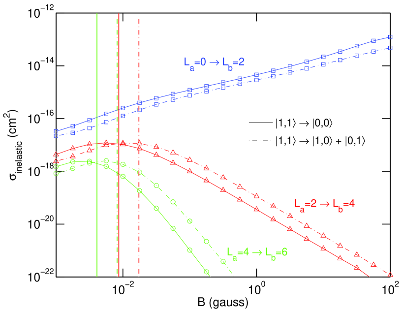
Figure 1: State-to-state collision cross sections for the $|M_{S_{A}}=1,M_{S_{B}}=1\rangle\rightarrow|M_{S_{A}}=0,M_{S_{B}}=0\rangle$ and $|M_{S_{A}}=1,M_{S_{B}}=1\rangle\rightarrow|M_{S_{A}}=1,M_{S_{B}}=0\rangle+|M_{S_{A}}=0,M_{S_{B}}=1\rangle$ transitions of NH + NH, obtained from full CC calculations as a function of magnetic field at $E=10^{-6}$ K. The (blue) lines marked with squares correspond to $L_{a}=0\rightarrow L_{b}=2$ transitions, the (red) lines marked with triangles correspond to $L_{a}=2\rightarrow L_{b}=4$, and the (green) lines marked with circles correspond to $L_{a}=4\rightarrow L_{b}=6$. The vertical lines indicate the $B_{c}$ values below which the crossings for $L_{a}=2\rightarrow L_{b}=4$ and $L_{a}=4\rightarrow L_{b}=6$ are energetically accessible.

As explained in Ref. Janssen et al. (2011b), the contribution from $V_{\rm{magn.dip}}$ is most easily understood by considering the adiabatic potential curves. We will repeat part of this discussion here for the sake of clarity. Asymptotically, the adiabatic curves correspond to the molecular eigenstates $\bar{\gamma}_{A}$ and $\bar{\gamma}_{B}$, and at finite $R$ each curve also contains a centrifugal barrier (see Fig. 1 of Ref. Janssen et al. (2011b)). Thus, at long range, the adiabats can be labeled by $|\bar{\gamma}_{A},\bar{\gamma}_{B}\rangle$ and $L$, and therefore also correlate to scattering channels. It has already been noted in Refs. Wallis et al. (2010) and Janssen et al. (2011b) that several adiabatic curves are narrowly avoided due to the intermolecular magnetic dipole interaction, and that the spin-flip induced by $V_{\rm{magn.dip}}$ takes place at the corresponding crossing. If we neglect the weak intramolecular spin-spin and spin-rotation couplings so that Eq. (II.2) holds, we can define the avoided-crossing points $R_{c}$ as

$$g_{S}\mu_{\rm{B}}B\Delta M_{S}=\frac{\hbar^{2}\left[L_{b}(L_{b}+1)-L_{a}(L_{a}+1)\right]}{2\mu R_{c}^{2}},$$ (58)

where $L_{a}$ and $L_{b}$ denote the values of $L$ for the adiabats correlating to the incoming and outgoing channels, respectively. The energies at which the crossings occur are given by

$$E_{c}=\frac{\hbar^{2}L_{a}(L_{a}+1)}{2\mu R_{c}^{2}},$$ (59)

defined relative to the threshold of the incident channel. We must point out that, since $V_{\rm{magn.dip}}$ contains a second-rank tensor in $\Omega_{R}$ and first-rank tensors in the monomer spin coordinates, the avoided crossings occur only if $L_{a}$ and $L_{b}$ differ at most by 2 and $M_{S_{i}}^{(a)}$ and $M_{S_{i}}^{(b)}$ ($i=A,B$) each differ at most by 1. Thus, not all crossings are avoided.

It can be deduced from Eq. (58) that, for small to moderate field strengths, the crossing points $R_{c}$ are located at very long range. Therefore, the spin-change due to $V_{\rm{magn.dip}}$ can occur without having to overcome the centrifugal barrier in the outgoing channel. More specifically, the $|M_{S_{A}}=M_{S_{B}}=1,L_{a}=0\rangle$ incident channel of NH–NH can couple with the $|M_{S_{A}}=1,M_{S_{B}}=0,L_{b}=2\rangle$ and $|M_{S_{A}}=M_{S_{B}}=0,L_{b}=2\rangle$ outgoing channels even at zero collision energy. Hence, at low energies and relatively low magnetic fields, the intermolecular magnetic dipolar interaction is the main source of trap loss for NH–NH.

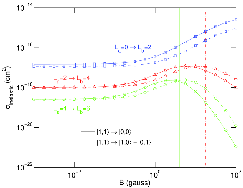
Figure 2: State-to-state collision cross sections for the $|M_{S_{A}}=1,M_{S_{B}}=1\rangle\rightarrow|M_{S_{A}}=0,M_{S_{B}}=0\rangle$ and $|M_{S_{A}}=1,M_{S_{B}}=1\rangle\rightarrow|M_{S_{A}}=1,M_{S_{B}}=0\rangle+|M_{S_{A}}=0,M_{S_{B}}=1\rangle$ transitions of NH + NH, obtained from full CC calculations as a function of magnetic field at $E=10^{-3}$ K. The (blue) lines marked with squares correspond to $L_{a}=0\rightarrow L_{b}=2$ transitions, the (red) lines marked with triangles correspond to $L_{a}=2\rightarrow L_{b}=4$, and the (green) lines marked with circles correspond to $L_{a}=4\rightarrow L_{b}=6$. The vertical lines indicate the $B_{c}$ values below which the crossings for $L_{a}=2\rightarrow L_{b}=4$ and $L_{a}=4\rightarrow L_{b}=6$ are energetically accessible.

It also follows from Eqs. (58) and (59) that the curve crossings for higher partial waves, e.g. for the $|M_{S_{A}}=M_{S_{B}}=1,L_{a}=2\rangle\rightarrow|M_{S_{A}}=M_{S_{B}}=0,L_{b}=4\rangle$ transition, become lower in energy as the magnetic field decreases. This implies that, at a fixed collision energy, the $L_{a}=2\rightarrow L_{b}=4$ channel transitions open up below a certain $B$-value. We will denote this critical magnetic field strength as $B_{c}$. Figures 1 and 2 show the state-to-state inelastic NH–NH cross sections for different $L_{a}\rightarrow L_{b}$ channel transitions as a function of $B$ at collision energies of 10^-6 K and 10^-3 K, respectively. The $B_{c}$ values for the $L_{a}=2\rightarrow L_{b}=4$ and $L_{a}=4\rightarrow L_{b}=6$ crossings are also indicated. For the $|M_{S_{A}}=M_{S_{B}}=1\rangle\rightarrow|M_{S_{A}}=M_{S_{B}}=0\rangle$ transitions, with $\Delta M_{S}=2$, the numerical values are $B_{c}=8.67\times 10^{-3}$ G at 10^-6 K and $B_{c}=4.09\times 10^{-3}$ G at 10^-3 K for $L_{a}=2\rightarrow L_{b}=4$, and $B_{c}=8.67$ G at 10^-6 K and $B_{c}=4.09$ G at 10^-3 K for $L_{a}=4\rightarrow L_{b}=6$. The critical field strengths for the $|M_{S_{A}}=M_{S_{B}}=1\rangle\rightarrow|M_{S_{A}}=1,M_{S_{B}}=0\rangle+|M_{S_{A}}=0,M_{S_{B}}=1\rangle$ transitions, with $\Delta M_{S}=1$, are twice as large as those for $\Delta M_{S}=2$. It can be seen that the inelastic cross sections for $L_{a}=2\rightarrow L_{b}=4$ and $L_{a}=4\rightarrow L_{b}=6$ indeed decrease as $B$ exceeds the corresponding $B_{c}$ value. This $B$-dependence is remarkable, considering that higher partial waves typically contribute only if the exothermicity in the outgoing channel is large. Due to the long-range nature of the magnetic dipole interaction, however, the scattering of higher partial waves becomes increasingly important as the exothermicity decreases, because the crossings points $R_{c}$ occur at a larger distance.

The influence of the kinetic energy on the inelastic cross section can also be understood in terms of the adiabatic curve crossings. For a given magnetic field strength, the avoided crossings for $L_{a}=2\rightarrow L_{b}=4$ and $L_{a}=4\rightarrow L_{b}=6$ are accessible only if the collision energy exceeds the $E_{c}$ value of Eq. (59). It followed from Eqs. (58) and (59) that, if $E_{c}$ increases, the critical field strength $B_{c}$ increases as well, and higher partial waves can contribute over an increasingly wide range of fields. This is also reflected in Figs. 1 and 2. In the ultracold regime, at a collision energy of 10^-6 K (Fig. 1), the $B_{c}$ values for $L_{a}=2\rightarrow L_{b}=4$ and $L_{a}=4\rightarrow L_{b}=6$ are relatively small and the $s$-wave incident channel ($L_{a}=0\rightarrow L_{b}=2$) is strongly dominant at all field strengths above $B\approx 10^{-2}$ G. At 10^-3 K, however, the $B_{c}$ values for the higher partial-wave channels are much larger, and we find that the $L_{a}=2$ and 4 incoming channels play a significant role at all magnetic field strengths below $B\approx 10$ G. A more detailed discussion on the energy dependence of the spin-inelastic cross section, based on the Born approximation, will be given in the next section.

III.2 Comparison with BA and DWBA

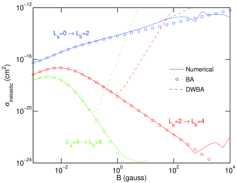
Figure 3: Total spin-inelastic collision cross sections for the $|M_{S_{A}}=1,M_{S_{B}}=1\rangle\rightarrow|M_{S_{A}}=0,M_{S_{B}}=0\rangle$ and $|M_{S_{A}}=1,M_{S_{B}}=1\rangle\rightarrow|M_{S_{A}}=1,M_{S_{B}}=0\rangle+|M_{S_{A}}=0,M_{S_{B}}=1\rangle$ transitions of NH + NH, calculated as a function of magnetic field at 10^-6 K. Different colors correspond to different $L_{a}\rightarrow L_{b}$ channel transitions.

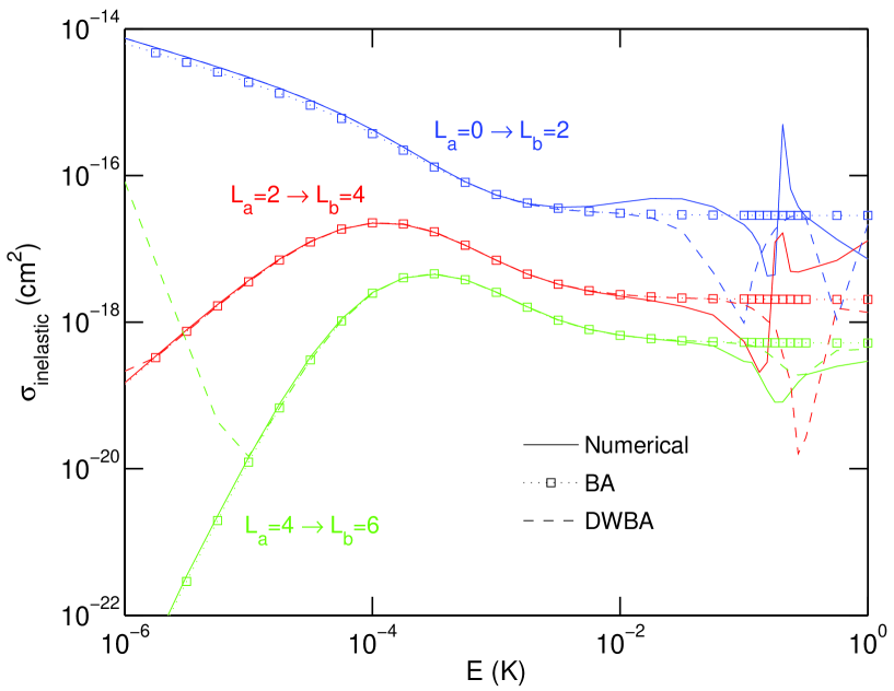
Figure 4: Total spin-inelastic collision cross sections for the $|M_{S_{A}}=1,M_{S_{B}}=1\rangle\rightarrow|M_{S_{A}}=0,M_{S_{B}}=0\rangle$ and $|M_{S_{A}}=1,M_{S_{B}}=1\rangle\rightarrow|M_{S_{A}}=1,M_{S_{B}}=0\rangle+|M_{S_{A}}=0,M_{S_{B}}=1\rangle$ transitions of NH + NH, calculated as a function of collision energy at a magnetic field strength of 1 G. Different colors correspond to different $L_{a}\rightarrow L_{b}$ channel transitions.

Before comparing our numerical results with the analytical BA and DWBA expressions, we must first point out that Eqs. (38) and (57) apply only to collisions in which $M_{S_{A}}$ and $M_{S_{B}}$ each change at most by 1 and $L$ changes at most by 2. Furthermore, the integral of Eq. (44) is defined only if $L_{b}>L_{a}+1$, and the DWBA cross section of Eq. (57) is therefore valid only for $L_{a}\rightarrow L_{a}+2$ transitions. Figure 3 shows the $|M^{(a)}_{S_{A}}=1,M^{(a)}_{S_{B}}=1,L_{a}\rangle\rightarrow|M^{(b)}_{S_{A}},M^{(b)}_{S_{B}},L_{a}+2\rangle$ cross sections as a function of $B$ at a collision energy of 10^-6 K. The cross sections are summed over all final states with $|M^{(b)}_{S_{A}}-M^{(a)}_{S_{A}}|\leq 1$ and $|M^{(b)}_{S_{B}}-M^{(a)}_{S_{B}}|\leq 1$. Figure 4 shows the results as a function of collision energy at a magnetic field strength of 1 G. It can be seen that the BA results are in very good agreement with the cross sections obtained from full CC calculations, in particular at low magnetic fields and low collision energies. At high fields and energies, the numerical cross sections exhibit several resonance features that arise mainly from the intramolecular spin-spin coupling term. Note that this coupling term is not included in the (DW)BA. Previous work has shown that the intramolecular spin-spin coupling becomes increasingly important as the kinetic energy in the outgoing channel increases, and, for $B>10^{2}$ G and $E>10^{-2}$ K, causes almost the same amount of spin relaxation as the intermolecular magnetic dipolar interaction Janssen et al. (2011b). Hence, the BA result of Eq. (38) deviates from the full CC result at high energies and field strengths.

It can also be seen in Figs. 3 and 4 that the analytical distorted-wave BA cross section, which contains an extra term due to the phase shift in the incoming channel, is in slightly better agreement with the numerical $L_{a}=0\rightarrow L_{b}=2$ cross section than the BA result. In particular, Fig. 3 shows that the BA cross section for $L_{a}=0\rightarrow L_{b}=2$ starts to deviate from the CC calculations around $B\approx 1$ G, while the DWBA is accurate up to $B\approx 100$ G. Thus, in the region between 1 and 100 G, the inelastic $L_{a}=0\rightarrow L_{b}=2$ cross section can be completely attributed to the intermolecular magnetic dipole interaction and to the phase shift in the incident channel. For the higher partial-wave channels, however, the analytical DWBA cross section deviates significantly from the full CC result at high fields and low energies. This is due to the $(k_{b}/k_{a})^{L_{a}+1}$ term in the expression for $\sigma^{\rm{DWBA}}_{a\rightarrow b}$ [Eq. (57)], which tends to infinity if $k_{a}\ll k_{b}$. Even for very small phase shifts, this term will dominate the DWBA inelastic cross section for $L_{a}>0$ if the collision energy is small and the exothermicity is large. More specifically, we estimate from Eq. (57) that the DWBA cross section diverges if $(k_{a}/k_{b})^{2L_{a}+1}\approx T^{(M_{a})}_{aa}$, and hence the effect is most pronounced for large $L_{a}$. We point out that the origin of the $(k_{b}/k_{a})^{L_{a}+1}$ term lies in the irregular spherical Bessel function $y_{L_{a}}(k_{a}R)$ [Eq. (44)], which enters the asymptotic wave function if the phase shift is nonzero. At short range, the $y_{L_{a}}$ function tends to infinity and ultimately leads to the unphysical behaviour observed in Figs. 3 and 4. A possible remedy for this problem is to evaluate the integral of Eq. (44) only for $R$-values larger than a certain cutoff radius. However, such an approach requires careful numerical analysis and falls out of the scope of the present study. Nevetheless, based on the results shown in Figs. 3 and 4, we conclude that the BA gives more meaningful results than the analytical DWBA at most of the energies and fields considered in this work. As a final point, we note that the numerical phase shifts for the higher partial-wave channels are orders of magnitude smaller than the $s$-wave scattering phase shift, and our DWBA results would not be substantially improved by including a phase shift in the outgoing channel.

As derived in Sec. II.2, the threshold behaviour of the BA spin-inelastic cross section in the limit of $k_{a}\ll k_{b}$ is given by $\sigma_{a\rightarrow b}\sim B^{1/2-L_{a}}$ and $\sigma_{a\rightarrow b}\sim E^{L_{a}-1/2}$. Indeed, we find that the $L_{a}=0\rightarrow L_{b}=2$, $L_{a}=2\rightarrow L_{b}=4$, and $L_{a}=4\rightarrow L_{b}=6$ inelastic cross sections at 10^-6 K behave as $B^{1/2}$, $B^{-3/2}$, and $B^{-7/2}$, respectively, for field strengths above $B\approx 5\times 10^{-2}$ G (see Fig. 3). Similarly, the cross sections at $B=1$ G follow an $E^{-1/2}$, $E^{3/2}$, and $E^{7/2}$ dependence, respectively, at collision energies below $E\approx 10^{-4}$ K (see Fig. 4). The validity regions of these threshold laws can also be explained in terms of the $V_{\rm{magn.dip}}$-induced avoided crossings discussed in Sec. III.1. The critical magnetic field strengths below which the $L_{a}=2\rightarrow L_{b}=4$ and $L_{a}=4\rightarrow L_{b}=6$ crossings are energetically accessible are on the order of $B_{c}\approx 10^{-2}$ G for a collision energy of 10^-6 K (see Fig. 1). If the magnetic field strength exceeds $B_{c}$, the crossings for the higher partial-wave channels are inaccessible and the corresponding scattering process can proceed only by (non-classical) tunneling through the centrifugal barrier. Hence we find the quantum-mechanical threshold behaviour at fields above $B\approx 10^{-2}$ G. For field strengths below $B_{c}$, the approximation of $k_{a}\ll k_{b}$ breaks down and the $B$-dependence follows from the explicit evaluation of Eq. (38). That is, the $B$-dependent threshold behaviour for $B<B_{c}$ is given by $(k_{a}/k_{b})^{2L_{a}-1}$ multiplied by the hypergeometric function. If the magnetic field is so small that $k_{a}\approx k_{b}$, the field dependence becomes negligible and the cross section flattens off to a constant value. In order to explain the energy dependence, we apply Eqs. (58) and (59) to determine the lowest possible $E_{c}$ values at which the avoided curve crossings can occur. At a magnetic field of 1 G, the corresponding values are $E_{c}=5.8\times 10^{-5}$ K for the $L_{a}=2\rightarrow L_{b}=4$ transition and $E_{c}=1.2\times 10^{-4}$ K for $L_{a}=4\rightarrow L_{b}=6$. Since the crossings for the higher partial-wave channels are inaccessible if $E<E_{c}$, we recover the quantum-mechanical threshold law at collision energies below $E\approx 10^{-4}$ K.

The results presented so far apply only to collisions where $M_{S_{A}}$ and $M_{S_{B}}$ decrease at most by 1 and $L$ increases by 2. The total spin-inelastic cross section, however, contains contributions from all (symmetry-allowed) outgoing partial waves and all final states, i.e. also the states with $M_{S_{A}}^{(b)}=-1$ and $M_{S_{B}}^{(b)}=-1$. Let us now compare the BA and DWBA results with the numerical total spin-inelastic cross sections for magnetically trapped NH ($M_{S_{A}}^{(a)}=M_{S_{B}}^{(a)}=1$), summed over all possible incoming partial waves and all outgoing channels. The total BA cross section is obtained by performing the sums over $L_{a}$ and $L_{b}$ in Eq. (38) for all possible (even) partial waves. To calculate the total DWBA cross section, we perform the sums over $L_{a}$ and $L_{b}$ in Eq. (57) for all possible (even) $L_{a}$ values and $L_{b}=L_{a}+2$. Since the numerical scattering calculations were carried out for $L_{\rm{max}}=6$, we also took this maximum value for $L_{a}$ and $L_{b}$ in the (DW)BA expressions.

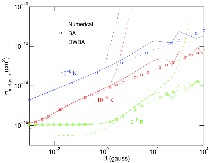
Figure 5: Total spin-inelastic collision cross sections for two magnetically trapped NH molecules, calculated as a function of magnetic field. Different colors correspond to different collision energies.

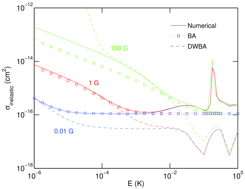
Figure 6: Total spin-inelastic collision cross sections for two magnetically trapped NH molecules, calculated as a function of collision energy. Different colors correspond to different magnetic field strengths.

The total inelastic cross sections are presented in Figs. 5 and 6. It can be seen that the BA is generally in much better agreement with the full CC result than the DWBA, except for a small region near 10 G at 10^-3 K (Fig. 5) and near 10^-3 K at 100 G (Fig. 6), where $k_{a}\approx k_{b}$. As noted previously, the deviation of the DWBA at high $B$ and low $E$ is due to the $(k_{b}/k_{a})^{L_{a}+1}$ term in Eq. (57), which causes unphysical behaviour if $k_{b}\gg k_{a}$. At low magnetic fields and relatively high energies, in particular at $E=10^{-3}$ K (see Fig. 5), we find that the DWBA cross section also deviates from the numerical result. In this region, the spin relaxation arises mainly from the $L_{a}=2\rightarrow L_{b}=2$ transition, and, to a smaller extent, also from the $L_{a}=0\rightarrow L_{b}=2$ and $L_{a}=2\rightarrow L_{b}=0$ transitions. Since the total DWBA cross section is restricted such that $L_{b}=L_{a}+2$, the most dominant inelastic transitions at low $B$ are thus not included in the DWBA. Similarly, the total DWBA cross section as a function of energy (Fig. 6) shows a clear discrepancy with the numerical result at $B=0.01$ G for nearly all energies considered, and at $B=1$ G for $E>10^{-3}$ K. This is also due primarily to the missing $L_{a}=2\rightarrow L_{b}=2$ channel transition.

It can also be seen that the total BA cross section, which does include all possible $L_{a}\rightarrow L_{b}$ transitions, agrees over a much wider range of $E$ and $B$, but deviates from the full CC result at high fields and high collision energies. As already discussed in the first paragraph of this section, the deviation partly arises from the intramolecular spin-spin coupling term, which contributes significantly to the numerical cross section as the kinetic energy in the outgoing channel becomes large. Moreover, the BA only includes contributions from final states with $M_{S_{A}}=0,1$ and $M_{S_{B}}=0,1$, while the total numerical cross section also contains terms with $M_{S_{A}}=-1$ and $M_{S_{B}}=-1$. Previous work has shown that, as the intramolecular spin-spin coupling term becomes increasingly important, the state-to-state cross sections for $M_{S_{A}}^{(b)}=-1$ and/or $M_{S_{B}}^{(b)}=-1$ increase as well Janssen et al. (2011b). Although the dominant mechanism for $M_{S_{i}}^{(a)}=1\rightarrow M_{S_{i}}^{(b)}=-1$ transitions is likely to be the intramolecular spin-spin term, which can decrease $M_{S_{i}}$ by 2 directly in first order, the intermolecular magnetic dipolar coupling term may also induce such spin-changing collisions in second order. This effect is included only in the full CC calculation, and hence this may represent another source of discrepancy between the BA and the numerical result.

IV Conclusions

We have presented a detailed theoretical study on the role of the intermolecular magnetic dipole-dipole interaction in (ultra)cold collisions of magnetically trapped NH($X\,^{3}\Sigma^{-}$) molecules. The inelastic cross sections for Zeeman relaxation have been obtained from rigorous coupled-channel calculations and from analytical results based on the (distorted-wave) Born approximation. The derived expressions for the analytical cross sections are valid for any two paramagnetic species for which the electronic spin and its space-fixed projection are (approximately) good quantum numbers, but we have applied them only to the NH + NH system.

We have found that the scattering of different partial waves, induced by the magnetic dipolar coupling, is most easily understood by considering the adiabatic potential curves. The intermolecular dipolar coupling term induces avoided crossings between certain adiabats at long range, which in turn may lead to Zeeman relaxation. The cross-section behaviour as a function of energy and magnetic field is, to a large extent, determined by whether or not these avoided crossings are energetically accessible. Remarkably, the avoided crossings for higher partial waves become lower in energy as the magnetic field strength decreases, implying that the corresponding channels open up below a certain critical field strength. Indeed, it was found that the scattering of higher partial waves becomes increasingly important as the exothermicity decreases.

The validity regions of the analytical BA and DWBA have been determined by comparison with numerical close-coupling calculations. We have found that the BA is accurate over a wide range of collision energies and fields, but starts to deviate from the numerical cross sections at energies above $\approx 10^{-2}$ K and fields above $\approx 10^{2}$ G. This is mainly due to the effect of the intramolecular spin-spin coupling term, which is neglected in the BA but contributes significantly to the numerical cross section as the kinetic energy in the outgoing channel becomes large. The analytical distorted-wave Born approximation, which accounts for a phase shift in the incident channel and thus represents a correction to the BA, gives more accurate results than the BA in the case of $s$-wave scattering. For higher partial-wave scattering, however, and in particular at high magnetic fields and low energies, the DWBA cross section shows unphysical behaviour and diverges to infinity. Furthermore, the derived DWBA expression is valid only for collisions where the partial-wave angular momentum is increased by 2, while the total numerical cross section contains contributions from all possible outgoing partial waves. More specifically, at fields below $\approx 1$ G and energies near 10^-3 K, the dominant contribution to the inelastic cross section is the $L_{a}=2\rightarrow L_{b}=2$ channel transition, which is not included in the DWBA. Hence we conclude that the BA, which contains all possible partial-wave contributions and does not show any unphysical behaviour, is generally in much better agreement with the full CC result than the DWBA.

Although we have focused only on NH(${}^{3}\Sigma^{-}$) + NH(${}^{3}\Sigma^{-}$) collisions in this study, the theory and main conclusions should be general for any two (ultra)cold paramagnetic species.