Thermoelectric and thermal transport in bilayer graphene systems

Abstract

We numerically study the disorder effect on the thermoelectric and thermal transport for bilayer graphene under a strong perpendicular magnetic field. In the unbiased case, we find that the thermoelectric transport has similar properties as in the monolayer graphene, i.e., the Nernst signal has a peak at the central Landau level (LL) with the value of the order of $k_{B}/e$ and changes sign near other LLs while the thermopower has an opposite behavior. We attribute this to the coexistence of particle and hole LLs around the Dirac point. When a finite interlayer bias is applied and a band gap is opened, it is found that the transport properties are consistent with those of a band insulator. We further study the thermal transport from electronic origins and verify the validity of the generalized Weidemann-Franz law.

I Introduction

Thermoelectric transport properties of graphene have attracted much recent experimental Kim09 ; Shi09 ; Ong08 and theoretical CastroNeto09 ; DasSarma09 ; Fogelstrom07 ; Thalmeier07 ; Ting09 ; Zhu10 attention. The thermopower (the longitudinal thermoelectric response) and the Nernst signal (the transverse response) in the presence of a strong magnetic field are found to be large, reaching the order of the quantum limit $k_{B}/e$, where $k_{B}$ and $e$ are the Boltzmann constant and the electron charge, respectively Kim09 ; Shi09 ; Ong08 . This has been attributed to the semi-metal type dispersion of graphene and/or in the vicinity of a quantum Hall liquid to insulator transition where the imbalance between the particle and hole types of carriers is significant. The thermoelectric effects are very sensitive to such an imbalance and become large in comparison with conventional metals.

In our previous study on graphene in the presence of disorder and an external magnetic field Zhu10 , we have shown that its thermoelectric transport properties are determined by the interplay of the unique band structure, the disorder-induced scattering, the Landau quantization and the temperature. While the band structure and the magnetic field determine the Landau level (LL) spectrum, the broadening of each LL is controlled by the competition between disorder-induced scattering and the thermal activation. We find that all transport coefficients are universal functions of $W_{L}/E_{F}$ and $k_{B}T/E_{F}$ when both $W_{L}$ and $k_{B}T$ are much smaller than the Landau quantization energy $\hbar\omega_{c}$. Here $W_{L}$, $E_{F}$ and $T$ are the disorder-induced LL broadening, the Fermi energy and the temperature, respectively. When $k_{B}T\ll W_{L}$, the thermoelectric conductivities vary as the density of states (and the particle-hole symmetry) is tuned by $E_{F}$ from the center of the LL to the mobility gap. When $k_{B}T\gg W_{L}$, thermal activation dominates and certain peak values for the thermopower $S_{xx}$ or the Nernst signal $S_{xy}$ reach universal numbers independent of the magnetic field or the temperature. While both $S_{xx}$ and $S_{xy}$ near high LLs ($\nu\neq 0$) have similar behaviors as those in two-dimensional (2D) semiconductor systems displaying the integer quantum Hall effect (IQHE) Girvin82 ; Streda83 ; Jonson84 ; Oji84 , they rather have opposite behaviors around the central LL. $S_{xy}$ has a peak while $S_{xx}$ vanishes and changes sign at the Dirac point ($E_{F}=0$). We have further argued that the unique behavior at the central LL is due to the coexistence of particle and hole LLs. As protected by the particle-hole symmetry, the contributions from particle and hole LLs cancel with each other exactly in the thermopower but superpose in the Nernst signal. The results for such a tight-binding analysis are in good agreement with experimental observations Kim09 ; Shi09 ; Ong08 .

In this work, we extend our study to bilayer graphene which has two parallel graphene sheets stacked on top of each other as in 3D graphite (the AB or Bernal stacking). While some common features are observed related to LLs with the same underlying particle-hole symmetry, bilayer graphene also demonstrates some interesting and different properties from monolayer graphene McCann06 ; Min07 ; Castro07 ; Oostinga08 ; Zhang09 ; Mak09 . The low energy dispersion of bilayer graphene can be effectively given by two hyperbolic bands $\epsilon_{k}\approx\pm k^{2}/(2m^{*})$ touching each other at the Dirac point ($E_{F}=0$), i.e., the electrons or holes have a finite mass $m^{*}$ which is in contrast to the massless excitations in monolayer graphene. Another important difference of bilayer graphene is the possibility to open up a band gap with a bias voltage, or a potential difference, applied between the two layers. This tunable gap system is advantageous to conventional semiconductor materials, making bilayer graphene more appealing from the point of view of applications. The thermoelectric transport properties of bilayer graphene are also expected to be interesting. The the thermopower of bilayer graphene without a magnetic field has been considered Hao10 . It is shown that as the density of states is also of the pseudogap type without a biased voltage, one expects that the relation for the thermopower $S_{xx}\sim T/E_{F}$ continues to hold. In addition, it is found that the room-temperature thermopower with a bias voltage can be enhanced by a factor of 4 than monolayer graphene or unbiased bilayer graphene Hao10 , making it a more promising candidate for future thermoelectric applications. Our study is to consider the thermopower and the Nernst effect under a magnetic field.

When an external magnetic field $B$ is applied, as in graphene and other IQHE systems, electron states of bilayer graphene are quantized into Landau levels. As the band dispersion changes, these LLs follow a different quantization sequence $E_{n}=\pm\sqrt{n(n-1)}\hbar\omega_{c}$ with $\omega_{c}\sim B$ rather than $\sqrt{B}$ for graphene. This has been confirmed by the theoretical E.McCann06 and experimental Novoselov06 studies on the quantum Hall effects, and further verified by our numerical calculation Ma08 . Compared with graphene, though the massive nature of particles and hyperbolic dispersion are different, the existence of the central LL ($\nu=0$) and the associated chiral and particle-hole symmetries are preserved. Therefore, the study on the thermoelectric transport in bilayer graphene not only provides theoretical predictions for their properties, in particular, their dependence on disorder and magnetic field for this system, but also helps to verify our argument on the central LL that its unique behavior is due to the chiral and particle-hole symmetries associated with the Dirac point.

For such purposes, we carry out a numerical study of the thermoelectric transport in both unbiased and biased bilayer graphene. We focus on studying the effects of disorder and thermal activation on the broadening of LLs and the corresponding thermoelectric transport properties. In the unbiased case, we indeed observe similar behaviors as in monolayer graphene for the central LL. Both the longitudinal and the transverse thermoelectric conductivities are universal functions of $W_{L}/E_{F}$ and $k_{B}T/E_{F}$ and display different asymptotic behaviors in different temperature regions. The calculated Nernst signal has a peak at the central LL with heights of the order of $k_{B}/e$, and changes sign near other LLs, while the thermopower has an opposite behavior. A higher peak value is obtained comparing to graphene due to the doubled degeneracy. This confirms our argument that as the particle and hole LLs coexist only in the central LL, the thermopower vanishes while the Nernst effect has a peak structure. As before, we verify the validity of the semiclassical Mott relation, which is shown to hold in a wide range of temperatures. When a bias is applied between the two graphene layers, the thermoelectric coefficients exhibit unique characteristics quite different from those of unbiased case. Around the Dirac point, the transverse thermoelectric conductivity exhibits a pronounced valley with $\alpha_{xy}=0$ at low temperature, and the thermopower displays a very large peak. We show that these features are associated with a band insulator, due to the opening of a sizable gap between the valence and conductance bands in biased bilayer graphene. In addition, we have calculated the thermal transport properties of electrons for both unbiased and biased bilayer graphene systems. In the biased case, it is found that the transverse thermal conductivity displays a pronounced plateau with $\kappa_{xy}=0$, which is accompanied by a valley in $\kappa_{xx}$. This provides additional evidence for the band insulator behaviors. We further compare the calculated thermal conductivities with those deduced from the Wiedemann-Franz law, to check the validity of this fundamental relation in graphene systems.

This paper is organized as follows. In Sec. II, we introduce the model Hamiltonian. In Sec. III and Sec. IV, numerical results based on exact diagonalization and thermoelectric transport calculations are presented for unbiased and biased systems, respectively. In Sec. V, numerical results for thermal transport are presented. The final section contains a summary.

II Model and Methods

We consider a bilayer graphene sample consisting of two coupled hexagonal lattices including inequivalent sublattices $A$, $B$ on the bottom layer and $\widetilde{A}$, $\widetilde{B}$ on the top layer. The two layers are arranged in the AB (Bernal) stacking S. B. Trickey ; K. Yoshizawa , where $B$ atoms are located directly below $\widetilde{A}$ atoms, and $A$ atoms are the centers of the hexagons in the other layer. Here, the in-plane nearest-neighbor hopping integral between $A$ and $B$ atoms or between $\widetilde{A}$ and $\widetilde{B}$ atoms is denoted by $\gamma_{AB}=\gamma_{\widetilde{A}\widetilde{B}}=\gamma_{0}$. For the interlayer coupling, we take into account the largest hopping integral between $B$ atom and the nearest $\widetilde{A}$ atom $\gamma_{\widetilde{A}B}=\gamma_{1}$, and the smaller hopping integral between an $A$ atom and three nearest $\widetilde{B}$ atoms $\gamma_{A\widetilde{B}}=\gamma_{3}$. The values of these hopping integrals are taken to be $\gamma_{0}=3.16$ eV, $\gamma_{1}=0.39$ eV, and $\gamma_{3}=0.315$ eV, as same as in Ref. Ma08 .

We assume that each monolayer graphene has totally $L_{y}$ zigzag chains with $L_{x}$ atomic sites on each chain Sheng06 . The size of the sample will be denoted as $N=L_{x}\times L_{y}\times L_{z}$, where $L_{z}=2$ is the number of monolayer graphene planes along the $z$ direction. We model charged impurities in substrate, randomly located in a plane at a distance $d$ from the graphene sheet with long-range Coulomb scattering potentials Adam08 . This type of disorder is known to give more satisfactory results for transport properties of graphene in the absence of a magnetic field Adam07 . When a magnetic field is applied perpendicular to the bilayer graphene plane, the Hamiltonian can be written in the tight-binding form

$$H_{0} = -\gamma_{0}(\sum\limits_{\langle ij\rangle\sigma}e^{ia_{ij}}c_{i\sigma}^{\dagger}c_{j\sigma}+\sum\limits_{\langle ij\rangle\sigma}e^{ia_{ij}}\widetilde{c}_{i\sigma}^{\dagger}\widetilde{c}_{j\sigma})$$ (1)

$$- \gamma_{1}\sum\limits_{\langle ij\rangle_{1}\sigma}e^{ia_{ij}}c_{j\sigma B}^{\dagger}\widetilde{c}_{i\sigma\widetilde{A}}-\gamma_{3}\sum\limits_{\langle ij\rangle_{3}\sigma}e^{ia_{ij}}c_{i\sigma A}^{\dagger}\widetilde{c}_{j\sigma\widetilde{B}}+h.c.$$

$$+ \sum\limits_{i\sigma}w_{i}(c_{i\sigma}^{\dagger}c_{i\sigma}+\widetilde{c}_{i\sigma}^{\dagger}\widetilde{c}_{i\sigma}),$$

where $c_{i\sigma}^{\dagger}$($c_{i\sigma A}^{\dagger}$), $c_{j\sigma}^{\dagger}$($c_{j\sigma B}^{\dagger}$) are creating operators on $A$ and $B$ sublattices in the bottom layer, and $\widetilde{c}_{i\sigma}^{\dagger}$($\widetilde{c}_{i\sigma\widetilde{A}}^{\dagger}$), $\widetilde{c}_{j\sigma}^{\dagger}$($\widetilde{c}_{j\sigma\widetilde{B}}^{\dagger}$) are creating operators on $\widetilde{A}$ and $\widetilde{B}$ sublattices in the top layer. $\sigma$ is a spin index. The sum $\sum_{\langle ij\rangle\sigma}$ denotes the intralayer nearest-neighbor hopping in both layers, $\sum_{\langle ij\rangle_{1}\sigma}$ stands for interlayer hopping between the $B$ sublattice in the bottom layer and the $\widetilde{A}$ sublattice in the top layer, and $\sum_{\langle ij\rangle_{3}\sigma}$ stands for the interlayer hopping between the $A$ sublattice in the bottom layer and the $\widetilde{B}$ sublattice in the top layer, as described above. The magnetic flux per hexagon $\phi=\sum_{{\small{\mbox{\hexagon}}}}a_{ij}=\frac{2\pi}{M}$ is proportional to the strength of the applied magnetic field $B$, where $M$ is assumed to be an integer and the lattice constant is taken to be unity. For charged impurities, $w_{i}=-\frac{Ze^{2}}{\epsilon}\sum_{\alpha}1/\sqrt{({\bf r}_{i}-{\bf R}_{\alpha})^{2}+d^{2}}$, where $Ze$ is the charge carried by an impurity, $\epsilon$ is the effective background lattice dielectric constant, and ${\bf r}_{i}$ and ${\bf R}_{\alpha}$ are the planar positions of site $i$ and impurity $\alpha$, respectively. All the properties of the substrate (or vacuum in the case of suspended graphene) can be absorbed into a dimensionless parameter $r_{s}=Ze^{2}/(\epsilon\hbar v_{F})$, where $v_{F}$ is the Fermi velocity of the electrons. For simplicity, in the following calculation, we fix the values of distance $d=1$nm and impurity density as $1\%$ of the total sites, and tune $r_{s}$ to control the impurity scattering strength.

For the biased system, the two graphene layers gain different electrostatic potentials, and the corresponding energy difference is given by $\Delta_{g}=\epsilon_{2}-\epsilon_{1}$ where $\epsilon_{1}=-\frac{1}{2}\Delta_{g}$, and $\epsilon_{2}=\frac{1}{2}\Delta_{g}$. The Hamiltonian can be written as: $H=H_{0}+\sum\limits_{i\sigma}\epsilon_{1}(c_{i\sigma}^{\dagger}c_{i\sigma}+\epsilon_{2}\widetilde{c}_{i\sigma}^{\dagger}\widetilde{c}_{i\sigma}$). For illustrative purpose, a relatively large asymmetric gap $\Delta_{g}=0.1\gamma_{0}$ is assumed, which is experimentally achievable Zhang09 .

In the linear response regime, the charge current in response to an electric field or a temperature gradient can be written as ${\bf J}={\hat{\sigma}}{\bf E}+{\hat{\alpha}}(-\nabla T)$, where ${\hat{\sigma}}$ and ${\hat{\alpha}}$ are the electrical and thermoelectric conductivity tensors, respectively. These transport coefficients can be calculated by Kubo formula once we obtain all the eigenstates of the Hamiltonian (in our calculation, $\sigma_{xx}$ is obtained based on the calculation of the Thouless number Ma08 ). In practice, we can first calculate the $T=0$ conductivities $\sigma_{ji}(E_{F})$, and then use the relation Jonson84

$$\sigma_{ji}(E_{F},T) = \int d\epsilon\,\sigma_{ji}(\epsilon)\left(-{\partial f(\epsilon)\over\partial\epsilon}\right),$$

$$\alpha_{ji}(E_{F},T) = {-1\over eT}\int d\epsilon\,\sigma_{ji}(\epsilon)(\epsilon-E_{F})\left(-{\partial f(\epsilon)\over\partial\epsilon}\right),$$ (2)

to obtain the finite temperature electrical and thermoelectric conductivity tensors. Here, $f(x)=1/[e^{(x-E_{F})/k_{B}T}+1]$ is the Fermi distribution function. At low temperatures, the second equation can be approximated as

$$\alpha_{ji}(E_{F},T)=-\frac{\pi^{2}k_{B}^{2}T}{3e}\left.\frac{d\sigma_{ji}(\epsilon,T)}{d\epsilon}\right|_{\epsilon=E_{F}},$$ (3)

which is the semiclassical Mott relation Jonson84 ; Oji84 . The thermopower and Nernst signal can be calculated subsequently from footnote1

$$S_{xx} = {E_{x}\over\nabla_{x}T}={\rho_{xx}\alpha_{xx}-\rho_{yx}\alpha_{yx}},$$

$$S_{xy} = {E_{y}\over\nabla_{x}T}={\rho_{xx}\alpha_{yx}+\rho_{yx}\alpha_{xx}}.$$ (4)

The thermal conductivity, measuring the magnitude of the thermal currents in response to an applied temperature gradient, includes electron and phonon contributions. In our numerical calculations, phonon-derived thermal conductivity is omitted. The electronic thermal conductivities $\kappa_{ji}$ at finite temperature assume the forms Oji84

$$\kappa_{ji}(E_{F},T) = {1\over e^{2}T}\int d\epsilon\,\sigma_{ji}(\epsilon)(\epsilon-E_{F})^{2}\left(-{\partial f(\epsilon)\over\partial\epsilon}\right)$$ (5)

$$- T\alpha_{ji}(E_{F},T)\sigma_{ji}^{-1}(E_{F},T)\alpha_{ji}(E_{F},T).$$

For diffusive electronic transport in metals, it is well known that the Wiedemann-Franz law is satisfied between the electrical conductivity $\sigma$ and the thermal conductivity $\kappa$ of electrons Ziman :

$${\kappa\over\sigma T}=L,$$ (6)

where L is the Lorentz number and takes a constant value: $L={\pi^{2}\over 3}({k_{B}\over e})^{2}$.

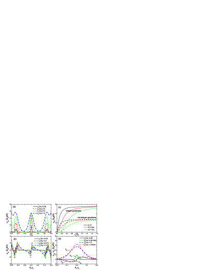
Figure 1: (color online). Thermoelectric conductivities at finite temperatures of bilayer graphene. (a)-(b) $\alpha_{xy}(E_{F},T)$ and $\alpha_{xx}(E_{F},T)$ as functions of the Fermi energy at different temperatures. (c) shows the temperature dependence of $\alpha_{xy}(E_{F},T)$ for monolayer and bilayer graphene. (d) compares the results from numerical calculations and from the generalized Mott relation at two characteristic temperatures, $k_{B}T/W_{L}=0.05$ and $k_{B}T/W_{L}=1$. The system size is taken to be $N=96\times 48\times 2$, magnetic flux $\phi=2\pi/48$, and disorder strength $r_{s}=0.3$ (we consider uniformly distributed positive and negative charged impurities within this strength) with $W_{L}/\gamma_{0}=0.0376$.

III Thermoelectric transport in unbiased bilayer graphene

We first show calculated thermoelectric conductivities at finite temperatures for unbiased bilayer graphene. As seen from Fig.1(a) and (b), the transverse thermoelectric conductivity $\alpha_{xy}$ displays a series of peaks, while the longitudinal thermoelectric conductivity ${\alpha_{xx}}$ oscillates and changes sign at the center of each LL. At low temperatures, the peak of $\alpha_{xy}$ at the central LL is higher and narrower than others, which indicates that the impurity scattering has less effect on the central LL. These results are qualitatively similar to those found in monolayer graphene Zhu10 due to the similar particle-hole symmetry in both cases, but some obvious differences exist. Firstly, the peak values of $\alpha_{xy}$ at the central LL is larger than that of monolayer graphene. Secondly, at low temperature, $\alpha_{xy}$ splits around $E_{F}=\pm 0.46\gamma_{0}$, which can be understood as due to the presence of $\nu=\pm 8$ Hall plateau by lifting subband degeneracy. In Fig.1(c), we find that $\alpha_{xy}$ shows different behavior depending on the relative strength of temperature $k_{B}T$ and the width of the central LL $W_{L}$($W_{L}$ is determined by the full-width at half-maximum of the $\sigma_{xx}$ peak). When $k_{B}T\ll W_{L}$ and $E_{F}\ll W_{L}$, $\alpha_{xy}$ shows linear temperature dependence, indicating that there is a small energy range where extended states dominate, and transport fall into the semi-classical Drude-Zener regime. When $E_{F}$ is shifted away from the Dirac point, the low temperature electron excitation is gapped related to Anderson-localization. When $k_{B}T$ becomes comparable to or greater than $W_{L}$, the $\alpha_{xy}$ for all LLs saturates to a constant value $5.54k_{B}e/h$. This matches exactly the universal number $(\ln 2)k_{B}e/h$ predicted for the conventional IQHE systems in the case where thermal activation dominates Jonson84 ; Oji84 , with an additional degeneracy factor $8$. The saturated value of $\alpha_{xy}$ in bilayer graphene is exactly twice than that of the monolayer graphene, as shown in Fig.1(c) in accordance with the eightfold degeneracy from valley, spin and layer degree of freedoms Novoselov06 ; E.McCann06 .

To examine the validity of the semiclassical Mott relation, we compare the above results with those calculated from Eq.(3), as shown in Fig.1(d). The Mott relation is a low-temperature approximation and predicts that the thermoelectric conductivities have linear temperature dependence. This is in agreement with our low-temperature results, which proves that the semiclassical Mott relation is asymptotically valid in Landau-quantized systems, as suggested in Ref. Jonson84 .

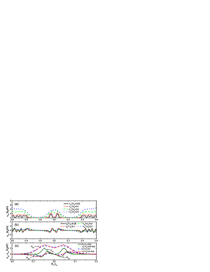
Figure 2: (color online). Thermoelectric conductivities at finite temperatures of biased bilayer graphene. (a)-(b) $\alpha_{xy}(E_{F},T)$ and $\alpha_{xx}(E_{F},T)$ as functions of the Fermi energy at different temperatures. (c) Compares the results from numerical calculations and from the generalized Mott relation at two characteristic temperatures, $k_{B}T/\Delta_{g}=0.05$ and $k_{B}T/\Delta_{g}=0.2$. Here asymmetric gap $\Delta_{g}=0.1\gamma_{0}$. The system size is taken to be $N=96\times 48\times 2$, magnetic flux $\phi=2\pi/48$, and disorder strength $r_{s}=0.3$.

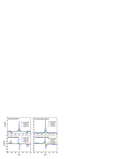
Figure 3: (color online). The thermopower $S_{xx}$ and the Nernst signal $S_{xy}$ as functions of the Fermi energy in (a)-(b)bilayer graphene, (c)-(d)biased bilayer graphene at different temperatures. All parameters in this two systems are chosen to be the same as in Fig. 1 and Fig. 2, respectively.

IV Thermoelectric transport in biased bilayer graphene

For biased bilayer graphene, we show results of $\alpha_{xx}$ and $\alpha_{xy}$ at finite temperatures in Fig. 2. Here we see that $\alpha_{xy}$ demonstrates a pronounced valley, in striking contrast to the unbiased case with a peak at the particle-hole symmetric point $E_{f}=0$. This behavior can be understood as due to the split of the valley degeneracy in the central LL by an opposite voltage bias added to the two layers. This is consistent with the opening of a sizable gap between the valence and conduction bands. More oscillations are observed in the higher LLs comparing to the unbiased case, in consistent with the further lifting of the LL degeneracy. ${\alpha_{xx}}$ oscillates and changes sign around the center of each split LL. In Fig.2(c), we also compare the above results with those calculated from the semiclassical Mott relation using Eq.(3). Here the Mott relation is shown to remain valid at low temperature.

We further calculate the thermopower $S_{xx}$ and the Nernst signal $S_{xy}$ using Eq. (4), which can be directly determined in experiments by measuring the responsive electric fields. In Fig. 3(a)-(b), we show results of $S_{xx}$ and $S_{xy}$ in unbiased bilayer graphene. As we can see, $S_{xy}$ ($S_{xx}$) has a peak at the central LL (the other LLs), and changes sign near the other LLs (the central LL), similar to the case of monolayer grapheneZhu10 . This oscillatory feature has been observed experimentally Lee10 . In our calculation, the peak value of $S_{xx}$ at $n=-1$ LL is found to be $14\mu V/K$ (note that $k_{B}/e=86.17\mu V/K$ ) for $k_{B}T=0.05W_{L}$ and $26\mu V/K$ for $k_{B}T=0.1W_{L}$, which is in good agreement with the measured value Lee10 . At zero energy, both $\rho_{xy}$ and $\alpha_{xx}$ vanish, leading to a vanishing $S_{xx}$. Around the zero energy, because $\rho_{xx}\alpha_{xx}$ and $\rho_{xy}\alpha_{xy}$ have opposite signs, depending on their relative magnitudes, $S_{xx}$ could either increases or decreases when $E_{F}$ is increased passing the Dirac point. In bilayer graphene, we find that $S_{xx}$ is always dominated by $\rho_{xy}\alpha_{xy}$, consequently, $S_{xx}$ decreases to negative value as $E_{F}$ passing zero. We find that the peak value of $S_{xx}$ in the central LL is $\pm 6\mu V/K$ at $k_{B}T=0.05W_{L}$. On the other hand, $S_{xy}$ has a peak structure at zero energy, which is dominated by $\rho_{xx}\alpha_{xy}$. The peak value is $42\mu V/K$ at $k_{B}T=0.05W_{L}$. These results are in good agreement with the experiments.

In Fig. 3(c)-(d), we show the calculated $S_{xx}$ and $S_{xy}$ in biased bilayer graphene system. As we can see, $S_{xy}$ ($S_{xx}$) has a peak around zero energy (the other LLs), and changes sign near the other LLs (zero energy). In our calculation, $S_{xx}$ is dominated by $\rho_{xx}\alpha_{xx}$, which is different from the unbiased bilayer graphene. At low temperature, the peak value of $S_{xx}$ around zero energy keeps almost unchanged around $\pm 181\mu V/K$, which is much larger than that of unbiased case. With the increase of temperature, the peak height increases to $\pm 396\mu V/K$ at $k_{B}T=0.5\Delta_{g}$. Theoretical study Hao10 indicates that, the large magnitude of $S_{xx}$ is mainly a result of the energy gap. On the other hand, $S_{xy}$ has a peak structure around zero energy, which is dominated by $\alpha_{xy}\rho_{xx}$. With $\sigma_{xx}\sim 2e^{2}/h$ near $E_{F}=0$, we find that the peak height is $198\mu V/K$ at $k_{B}T=0.1\Delta_{g}$, which is larger than that of unbiased case.

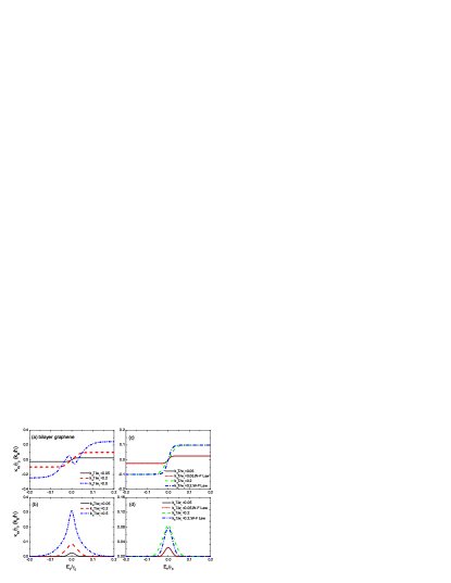
Figure 4: (color online). (a)-(b) Thermal conductivities $\kappa_{xy}(E_{F},T)$ and $\kappa_{xx}(E_{F},T)$ as functions of the Fermi energy in bilayer graphene at different temperatures, (c)-(d)Compares the thermal conductivity as functions of the Fermi energy from numerical calculations and from the Wiedemann-Franz Law at two characteristic temperatures. The parameters chosen here are the same as in Fig. 1.

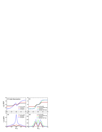
Figure 5: (color online). (a)-(b) Thermal conductivities $\kappa_{xy}(E_{F},T)$ and $\kappa_{xx}(E_{F},T)$ as functions of the Fermi energy in biased bilayer graphene at different temperatures, (c)-(d)Compares the thermal conductivity as functions of the Fermi energy from numerical calculations and from the Wiedemann-Franz Law at two characteristic temperatures. The parameters chosen here are the same as in Fig. 2.

V Thermal conductivity for unbiased and biased bilayer graphene systems

We now focus on thermal conductivities. In Fig. 4, we show results of the transverse thermal conductivity $\kappa_{xy}$ and the longitudinal thermal conductivity $\kappa_{xx}$ for unbiased bilayer graphene at different temperatures. As seen from Fig.4(a) and (b), $\kappa_{xy}$ exhibits two flat plateaus away from the center of the central LL. At low temperatures, the transition between these two plateaus is smooth and monotonic, while at higher temperatures, $\kappa_{xy}$ exhibits an oscillatory feature at $k_{B}T=0.5W_{L}$ between two plateaus. On the other hand, $\kappa_{xx}$ displays a peak near the center of the central LL, while its peak value increases quickly with $T$. To test the validity of the Wiedemann-Franz Law, we compare the above results with ones calculated from Eq.(6) as shown in Fig.4(c) and (d). The Wiedemann-Franz Law predicts that the ratio of the thermal conductivity $\kappa$ to the electrical conductivity $\sigma$ of a metal is proportional to the temperature. This is in agreement with our low-temperature results, while deviation is seen at higher $T$.

In Fig. 5, we show the calculated thermal conductivities $\kappa_{xx}$ and $\kappa_{xy}$ for biased bilayer graphene. As seen from Fig.5(a) and (b), around the zero energy, a flat region with $\kappa_{xy}=0$ is found at low temperatures, which is accompanied by a valley in $\kappa_{xx}$. These features are clearly in contrast to those of unbiased case due to the asymmetric gap between the valence and conduction bands. When temperature increases to $k_{B}T=0.2\Delta_{g}$, the plateau with $\kappa_{xy}=0$ disappears, while $\kappa_{xx}$ displays a large peak. In Fig.5(c) and (d), we also compare above results with those calculated from the Wiedemann-Franz Law using Eq.(6). Due to the presence of energy gap, we find that the Wiedemann-Franz Law is not valid in the biased bilayer graphene.

VI Summary

In summary, we have numerically investigated the thermoelectric and thermal transport in unbiased bilayer graphene based on the tight-binding model in the presence of both disorder and magnetic field. We find that the thermoelectric conductivities display different asymptotic behaviors depending on the ratio between the temperature and the width of the disorder-broadened Landau levels (LLs), similar to those found in monolayer graphene. In the high temperature regime, the transverse thermoelectric conductivity $\alpha_{xy}$ saturates to a universal quantum value $5.54k_{B}e/h$ at the center of each LL, and it has a linear temperature dependence at low temperatures. The calculated Nernst signal $S_{xy}$ has a peak at the central LL with heights of the order of $k_{B}/e$, and changes sign at the other LLs, while the thermopower $S_{xx}$ has an opposite behavior. These results are in good agreement with the experimental observationLee10 . The validity of the semiclassical Mott relation between the thermoelectric and electrical transport coefficients is verified in a range of temperatures. The calculated transverse thermal conductivity $\kappa_{xy}$ exhibits two plateaus away from the band center. The transition between this two plateaus is continuous, which is accompanied by a pronounced peak in longitudinal thermal conductivity $\kappa_{xx}$. The validity of the Wiedemann-Franz Law between the thermal conductivity $\kappa$ and the electrical conductivity $\sigma$ is only verified at very low temperatures.

We further discuss the thermoelectric transport of biased bilayer graphene. When a bias is applied to the two graphene layers, the thermoelectric coefficients exhibit unique characteristics different from those of unbiased case. Around the Dirac point, transverse thermoelectric conductivity exhibits a pronounced valley with $\alpha_{xy}=0$ at low temperatures, and the thermopower displays a large magnitude peak. Furthermore, the transverse thermal conductivity has a pronounced plateau with $\kappa_{xy}=0$, which is accompanied by a valley in $\kappa_{xx}$. These are in consistent with the opening of sizable gap between the valence and conductance bands in biased bilayer graphene.

We mention that in our numerical calculations, the magnetic field is much stronger than the ones one can realize in the experimental situation, as limited by current computational capability. However, the asymptotic behaviors we obtained is robust and applicable to weak field limit since it is determined by the topological property of the energy band as clearly established for monolayer graphene Zhu10 .

- (1) Y.M. Zuev, W. Chang, and P. Kim, Phys. Rev. Lett. 102, 096807 (2009).
- (2) P. Wei, W. Bao, Y. Pu, C. N. Lau, and J. Shi, Phys. Rev. Lett. 102, 166808 (2009).
- (3) J.G. Checkelsky and N.P. Ong, Phys. Rev. B 80, 081413(R) (2009).
- (4) A. H. Castro Neto, F. Guinea, N. M. R. Peres, K. S. Novoselov and A. K. Geim, Rev. Mod. Phys. 81, 109 (2009).
- (5) E. H. Hwang, E. Rossi, and S. Das Sarma, Phys. Rev. B 80, 235415 (2009).
- (6) T. Löfwander and M. Fögelstrom, Phys.Rev. B 76, 193401 (2007).
- (7) B. Dóra and P. Thalmeier, Phys. Rev. B 76, 035402 (2007).
- (8) X.-Z. Yan, Y. Romiah, and C. S. Ting, Phys. Rev. B 80, 165423 (2009).
- (9) L. Zhu, R. Ma, L. Sheng, M. Liu, and D. N. Sheng, Phys. Rev. Lett. 104, 076804 (2010).
- (10) S. M. Girvin and M. Jonson, J. Phys. C 15, L1147(1982).
- (11) P. Středa, J. Phys. C 16, L369 (1983).
- (12) M. Jonson and S.M. Girvin, Phys. Rev. B 29, 1939 (1984).
- (13) H. Oji, J. Phys. C 17, 3059 (1984).
- (14) E. McCann, Phys. Rev. B 74, 161403(R) (2006).
- (15) H. Min, B. Sahu, S. K. Banerjee, and A. H. MacDonald, Phys. Rev. B 75, 155115 (2007).
- (16) E. V. Castro, K. S. Novoselov, S. V. Morozov, N. M. R. Peres, J. M. B. Lopes dos Santos, J. Nilsson, F. Guinea, A. K. Geim, and A. H. Castro Neto, Phys. Rev. Lett. 99, 216802 (2007).
- (17) J. B. Oostinga, H. B. Heersche, X. Liu, A. F. Morpurgo, and L. M. K. Vandersypen, Nat. Mater. 7, 151 (2008).
- (18) Y. Zhang, T.-T. Tang, C. Girit, Z. Hao, M. C. Martin, A. Zettl, M. F. Crommie, Y. R. Shen, and F. Wang, Nature 459, 820 (2009).
- (19) K. F. Mak, C. H. Lui, J. Shan, and T. F. Heinz, Phys. Rev. Lett. 102, 256405 (2009).
- (20) L. Hao and T. K. Lee, Phys. Rev. B 81, 165445 (2010).
- (21) E. McCann and V. I. Fal’ko, Phys. Rev. Lett. 96, 086805 (2006).
- (22) K. S. Novoselov, E. McCann, S. V. Morozov, V. I. Fal’ko, M. I. Katsnelson, U. Zeitler, D. Jiang, F. Schedin and A. K. Geim, Nature Phys. 2, 177 (2006).
- (23) R. Ma, L. Sheng, R. Shen, M. Liu and D. N. Sheng, Phys. Rev. B 80, 205101 (2009); R. Ma, L. Zhu, L. Sheng, M. Liu, D. N. Sheng, Europhys. Lett. 87, 17009 (2009).
- (24) S. B. Trickey, F. M .. u ller-Plathe, and G. H. F. Diercksen, Phys. Rev. B 45, 4460 (1992).
- (25) K. Yoshizawa, T. Kato, and T. Yamabe, J. Chem. Phys. 105, 2099 (1996); T. Yumura and K. Yoshizawa, Chem. Phys. 279, 111 (2002).
- (26) D.N. Sheng, L. Sheng, and Z.Y. Weng, Phys. Rev. B 73, 233406 (2006).
- (27) S. Adam and S. Das Sarma, Solid State Communications 146,356 (2008).
- (28) S. Adam, E. H. Hwang, V. M. Galitski, and S. Das Sarma, Proc. Natl. Acad. Sci. USA 104, 18392 (2007).
- (29) Different literatures may have a sign difference due to different conventions.
- (30) J. M. Ziman, Electrons and Phonons (Oxford University Press,
- (31) S.G. Nam, D.K. Ki, H.J. Lee, Phys. Rev. B 82, 245416 (2010).