Nondeterminstic ultrafast ground state cooling of a mechanical resonator

Abstract

We present an ultrafast feasible scheme for ground state cooling of a mechanical resonator via repeated random time-interval measurements on an auxiliary flux qubit. We find that the ground state cooling can be achieved with several such measurements. The cooling efficiency hardly depends on the time-intervals between any two consecutive measurements. The scheme is also robust against environmental noises.

Introduction.– In the quantum regime, ground state cooling of a small thermal object is an intriguing challenge and one of the most desirable quantum technologies. Physically, the cooling process can be formulated as a transformation from a thermal state of the small object into its ground state. The transformation is irreversible and cannot be performed when the object is isolated.

A mechanical resonator (MR) is a small mecroscopic mechanical object, usually coupled to an auxiliary setup. The physical realization of its quantum ground state has become more and more important in ultrahigh-precision measurements, classical to quantum transitions, preparations of non-classical states, quantum information processing ultrahigh detection ; quantum-mechanical ; QIP-MR . Throughout the years, considerable number of optomechanical Metzger:2004 ; Thompson:2007 ; Wilson-Rae:2007 ; Marquardt:2007 ; Li-Cooling ; Kippenberg2007 ; Li-2010 and electromechanical electromechanical-1 ; Zhang-PRL ; electromechanical-3 ; electromechanical-4 ; Jacobs-2010 ; cooling-in-TLR models has been proposed for achieving their ground state cooling. Examples are a bang-bang cooling through a Cooper pair box Zhang-PRL , a single-shot state-swapping cooling via the superconductor via a superconductor Jacobs-2010 . Recently, some of us Li-2010 proposed a ground state cooling scheme of MR in an optomechanical system by controlling fast the optical drives. The best studied ground state cooling protocol is the sideband cooling Metzger:2004 ; Wilson-Rae:2007 ; Marquardt:2007 ; Li-Cooling ; Kippenberg2007 designed originally for cooling the atomic spatial motion. This cooling is now widely used for the MR cooling experiments and the recent record for the mean phonon number is $3.8$ cooling-in-TLR Theoretically, a MR could be cooled down to its ground state in the resolved sideband limit, with the mean phonon number less than 1. Since ground state cooling is not yet achieved experimentally and seems to become much harder when close to ground state, new cooling approaches remain desired.

This work presents a new protocol for MR cooling using repeated projective measurements on an auxiliary qubit. While it may be used in any stage of the cooling process of a MR, our protocol is aimed at the ground state cooling. Our study starts with the cooling with repeated equal time-interval measurements on the qubit, introduced for purification of quantum states purification or measurement-based entanglement generation Wu-PRA04 ; Plenio-PRA99 . While equal time-interval repeated measurements work well for ground state cooling, we find, unexpectedly, that the cooling efficiency is even much better when the repeated measurements are taken randomly. The ground state can be reached in several such measurements in very short time. We give explanation on the unexpected phenomenon. These results suggest that our protocol is completely robust against measurement operational errors. In addition to this great advantage, the scheme is also robust against environmental noises.

Figure 1: (Color online) Schematic diagram of the circuit. The top left part (red) is the coupled flux qubit-MR system, where each cross denotes a Josephson junction and the bar denotes a doubly-clamped MR. The interaction between MR and flux qubit is modulated by an in-plane magnetic field $B_{0}$. The top right part (blue) is a Josephson bifurcation amplifier (JBA) formed by a dc SQUID shunted by a capacitance. The bottom part (green) is bias to control the qubit energy gap as well as the coupling strength between the JBA and the qubit.

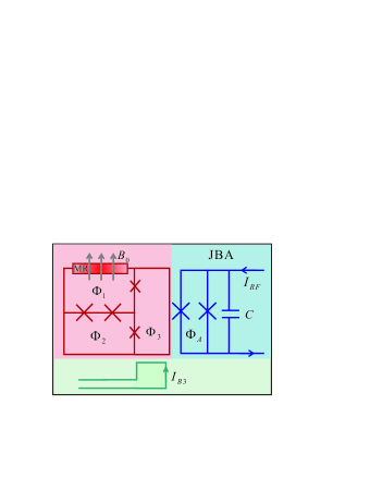
Model.– We employ a gradiometer-type flux qubit Paauw et al. (2009); Fedorov et al. (2010) as our auxiliary qubit, though our scheme may be applicable to any two-level system coupled to a MR. Fig. 1 is a schematic diagram of our cooling setup. The doubly-clamped MR (the red bar in Fig. 1), is embedded in a flux qubit circuit which composed of three superconducting loops with four Josephson junctions (JJs). An in-plane magnetic field $B_{0}$ induces qubit-MR coupling via Lorentz force Fei Xue . The top right blue (bottom green) part is to measure (operate) the qubit as described later.

The Hamiltonian of the flux qubit can be written as $H_{q}={\hbar\Delta}\sigma_{x}/{2}+{\hbar\epsilon}\sigma_{z}/{2}$, where $\sigma_{z}$ and $\sigma_{x}$ are the Pauli matrices in the basis of two persistent current states $\left|\uparrow\right\rangle$ and $\left|\downarrow\right\rangle$. Here, $\hbar\Delta$ is the tunneling amplitude between the two states. The bias energy $\hbar\epsilon$ linearly depends on external flux bias and in our case is set to zero by pre-trapping one flux quantum $\Phi_{0}$ in the loop Paauw et al. (2009); Fedorov et al. (2010).

The MR is modeled as a single-mode harmonic oscillator with a high-$Q$ mode of frequency $\omega_{m}$ and effective mass $m$. The entire system is characterized by the Hamiltonian Fei Xue

$$H=H_{q}+\hbar\omega_{m}a^{\dagger}a-\hbar g(a+a^{\dagger})\sigma_{z},$$ (1)

where $a$ and $a^{\dagger}$ are annihilation and creation operators for the MR with frequency $\omega_{m}$. The last term denotes the interaction between the MR and the flux qubit. The coupling constant is $g=B_{0}I_{p}L_{0}$ with $B_{0}$ the magnitude of the in-plane magnetic field, $I_{p}$ the magnitude of the persistent current in the loop, and $L_{0}$ the length of the MR.

Here we consider a MR with fundamental mode frequency $\omega_{m}\sim 2\pi\times 100$ MHz. The qubit is tuned into resonance or near resonance with the MR by monitoring the tunneling $\Delta$ Fedorov et al. (2010); Zhu et al. (2010). The coupling constant $g$, e.g., $\sim 2\pi\times 1$ MHz, is much smaller than the qubit frequency such that the rotating wave approximation (RWA) can be used to reduce the Hamiltonian Eq. (1) to the standard Jaynes-Cummings (JC) Hamiltonian

$$H=\hbar\omega_{m}a^{\dagger}a+\frac{\hbar\Delta}{2}\tilde{\sigma}_{z}+\hbar g(a\tilde{\sigma}_{+}+a^{\dagger}\tilde{\sigma}_{-}),$$ (2)

where $\tilde{\sigma}_{z,\pm}$ are the Pauli operators in the new basis of ground and excited states: $\left|g/e\right\rangle=(\left|\downarrow\right\rangle+/-\left|\uparrow\right\rangle)/\sqrt{2}$.

The operator $\hat{N}_{c}=a^{\dagger}a+\left|e\right\rangle\left\langle e\right|$ in the JC model is conserved, such that $H$ can be represented by the direct sum of a one-dimensional block in the basis $\left|0,g\right\rangle$ and two-dimensional submatrices in pairs of bases $\left|n,g\right\rangle$ and $\left|n-1,e\right\rangle$ when $n\geq 1$. The Hamiltonian (2) can be therefore diagonalized (we set $\hbar=1$)

$$H=-\frac{\Delta}{2}\left|0,g\right\rangle\left\langle 0,g\right|+\sum_{n\geq 1}\sum_{s=\pm}\varepsilon_{n}^{s}\left|ns\right\rangle\left\langle ns\right|,$$ (3)

where the dressed eigenstates $\left|n+\right\rangle=\cos\theta_{n}\left|n-1,e\right\rangle+\sin\theta_{n}\left|n,g\right\rangle,$ $\left|n-\right\rangle=\sin\theta_{n}\left|n-1,e\right\rangle-\cos\theta_{n}\left|n,g\right\rangle$ and the corresponding eigenvalues are $\varepsilon_{n}^{\pm}=(n-1/2)\omega_{m}\pm\sqrt{(\Delta-\omega_{m})^{2}/4+g^{2}n}$. Here $\theta_{n}$ satisfies the equation $\tan 2\theta_{n}=2g\sqrt{n}/(\Delta-\omega_{m})$ for $n\geq 1$.

Unitary evolution and repeated measurements.– We prepare the whole system initially in a separable state, $\rho_{0}=\left|g\right\rangle\left\langle g\right|\otimes\rho_{m}$. Here $\rho_{m}$ is the thermal state of the MR (it could also be an arbitrary state, where the MR ground state $\left|0\right\rangle$ is included). We then perform repeated but unequal time-interval measurements (UTIMs) on the flux qubit. The whole system evolves under the JC Hamiltonian (2) in between the measurements. The $j$-th measurement takes place at the time instant $t_{j}=j\tau+\delta t_{j}$, where $\tau$ is a given time interval and $\delta t_{j}$’s are random variations in time in the interval $(-\tau/2,\tau/2)$. The time interval between the $(j-1)$-th and $j$-th measurements is unequal, $\tau_{j}=\tau+\delta t_{j}-\delta t_{j-1}$ (for $j\geq 1$ and $t_{0}=\delta t_{0}\equiv 0$). When all $\delta t_{j}\equiv 0$, the repeated process is reduced into equal time-interval measurements (ETIMs) formulated in purification . After $N$ such ETIMs on the qubits and if all measurement outcomes are $\left|g\right\rangle$, the density matrix of the MR becomes $\rho_{m}^{(\tau)}(N)=V_{g}^{N}(\tau)\rho_{m}V_{g}^{\dagger N}(\tau)/P_{g}^{(\tau)}(N)$, where $P_{g}^{(\tau)}(N)={\mathrm{Tr}}[V_{g}^{N}(\tau)\rho_{m}V_{g}^{\dagger N}(\tau)]$ is the survival probability purification ; Wu-PRA . Here $V_{g}(\tau)\equiv\left\langle g\right|e^{-iH\tau/\hbar}\left|g\right\rangle$ is an effective evolution operator only acting on the MR.

$V_{g}(\tau)$ for model (2) is diagonal in the basis {$\left|n\right\rangle$}: $V_{g}(\tau)=\sum_{n\geqslant 0}\lambda_{n}(\tau)\left|n\right\rangle\left\langle n\right|$. Here the eigenvalues are $\lambda_{0}=e^{i{\Delta}\tau/{2}}$ and $\lambda_{n}=e^{-i(n-1/2)\omega_{m}\tau}(\cos\Omega_{n}\tau+i\sin\Omega_{n}\tau\cos 2\theta_{n})$ with $\Omega_{n}=\sqrt{(\Delta-\omega_{m})^{2}/4+g^{2}n}$ for $n\geq 1$. By carefully selecting the time interval $\tau$ such that $\cos^{2}\Omega_{n}\tau\neq 0$ (for $n\geq 1$), all the values

$$|\lambda_{n}(\tau)|\ =\sqrt{1-\cos^{2}\Omega_{n}\tau\cos^{2}2\theta_{n}}$$ (4)

can be made less than $1$, while $|\lambda_{0}(\tau)|$ always equals to $1$.

In the large $N$ limit for our specific JC model, the UTIMs result in

$$V_{g}(\tau_{1})V_{g}(\tau_{2})...V_{g}(\tau_{N})=\sum_{n\geqslant 0}|\bar{\lambda}_{n}|^{2N}\left|n\right\rangle\left\langle n\right|\rightarrow\left|0\right\rangle\left\langle 0\right|,$$

where $|\bar{\lambda}_{n}|^{2}=\left(\left|\lambda_{n}(\tau_{1})\right|^{2}\left|\lambda_{n}(\tau_{2})\right|^{2}...\left|\lambda_{n}(\tau_{N})\right|^{2}\right)^{1/N}<1$ for $n\geq 1$ and $|\bar{\lambda}_{0}|=1$. All the density matrix elements of the MR will vanish, except that of ground state $\left|0\right\rangle$:

$$\rho_{m}^{(\tau)}(N) =\sum_{n\geq 0}|\bar{\lambda}_{n}|^{2N}\rho_{m}^{(n)}\left|n\right\rangle\left\langle n\right|/P_{g}^{(\tau)}(N)$$ (5)

$$\rightarrow\left|0\right\rangle\left\langle 0\right|,~{}~{}\mathrm{for}~{}N\rightarrow\infty,$$

where $\rho_{m}^{(n)}\equiv\left\langle n\right|\rho_{m}\left|n\right\rangle$ and the survival probability $P_{g}^{(\tau)}(N)=\sum_{n\geqslant 0}|\bar{\lambda}_{n}|^{2N}\rho_{m}^{(n)}\rightarrow\rho_{m}^{(0)}$. For the case of ETIMs, $|\bar{\lambda}_{n}|=\left|\lambda_{n}(\tau)\right|$. Repeated measurements drive the evolution from the initial state (e.g., the thermal state) to the ground state of a MR. The process has the same features as those of known ground state cooling methods and is a new method for ground state cooling of a MR. Furthermore, distinct from usual dynamical cooling schemes, the new cooling method is based on repeated non-dynamical measurements.

Figure 2: (Color online) (a) The average phonon number $\bar{n}(N)$ after $N$ equal time-interval measurements (ETIMs) for the initial phonon number $\bar{n}(0)=3.69$. (b) The corresponding survival probability $P_{g}^{(\tau)}(N)$ and fidelity $F_{g}^{(\tau)}(N)$ (inset). The gray square lines denote the resonant case $\Delta=\omega_{m}$. The red triangle lines denote the non-resonant case $\Delta=1.1\omega_{m}$. Here $g=0.04\omega_{m}$ and $\tau=10/\omega_{m}$.

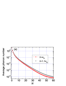
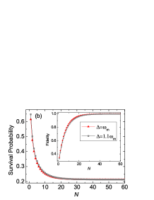
Numerical results and robustness.– Consider a $2\pi\times 100$ MHz nano-mechanical resonator with quality factor $Q_{m}=10^{5}$ ($\gamma_{m}/2\pi=200$ Hz), coupled to a flux qubit with the tunneling splitting $\Delta\simeq\omega_{m}$. The MR is initially at its thermal equilibrium state at the ambient temperature $T=20$ mK, and the corresponding mean phonon number is $\bar{n}(0)=1/[{{\exp(\hbar\omega_{m}/k_{B}T})-1}]=3.69$. Fig. 2 shows for ETIMs the mean phonon number $\bar{n}(N)$, the survival probability $P_{g}^{(\tau)}(N)$, and the fidelity $F_{g}^{(\tau)}(N)\equiv\left\langle 0\right|\rho_{m}^{(\tau)}(N)\left|0\right\rangle$ as a function of $N$, the number of measurements. The lines with red triangles in Fig. 2 are for the on-resonant $\Delta=\omega_{m}$ case and the lines with gray squares correspond to the off-resonant case, $\Delta=1.1\omega_{m}$. The ground state cooling can be reached in both cases. Fig. 2 shows that while the ground state cooling requires $60$ measurements ($\bar{n}(N=60)\approx 10^{-4}$), the mean phonon number decreases $90$ percent with only five measurements.

Figure 3: (Color online) The average phonon number $\bar{n}(N)$ (a), the survival probability (b), and the fidelity [inset in (b)], after $N$ measurements in the resonant case $\Delta=\omega_{m}$. The lines with red triangles denote the equal time-interval measurements (ETIMs) ($\tau=8/\omega_{m}$) and the lines with blue circles denote the unequal time-interval measurements (UTIMs) note1 . Here the initial phonon number $\bar{n}(0)=7.84$, and the coupling strength $g=0.04\omega_{m}$.

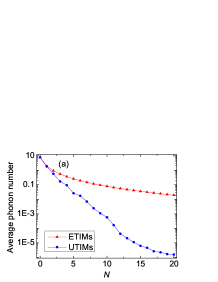
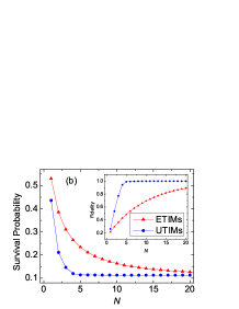
The ideal ETIMs, with time interval $\tau$, may be difficult technically. Fig. 3 shows, for UTIMs, the same physical quantities as Fig. 2 for the $\Delta=\omega_{m}$ case, but with the higher bath temperature $T=40$ mK and randomly selected time intervals $\tau_{j}$. The mean phonon number is $\bar{n}(0)=7.84$ initially. It is noticeable that the ground state cooling can be achieved much more efficiently than the ETIMs. It is a remarkable advantage for experimentalists to achieve the ground state cooling of MRs with random time intervals.

The physical reason is clear. In general, for a fixed $n$, the smaller the maximal value $\Lambda_{n}=\max\{\left|\lambda_{n}(\tau_{j})\right|\}_{j=1,...,N}$ is, the faster the term $|\bar{\lambda}_{n}|^{2N}\left|n\right\rangle\left\langle n\right|$ decays with $N$. For ETIMs, it is unavoidable that there exists $\Lambda_{n}$ ($n\geq 1$) very close to one, since for a given finite time interval $\tau$ the periodical function $\cos(\Omega_{n}\tau)$ versus $\Omega_{n}$ runs across $0$ several times. The corresponding component $\left|n\right\rangle\left\langle n\right|$ therefore decays very slowly. Specially, the component $\left|n\right\rangle\left\langle n\right|$ will not decay with $N$ for ETIMs when $\Lambda_{n}=1$. However for random UTIMs, the corresponding $|\bar{\lambda}_{n}|^{2N}\left|n\right\rangle\left\langle n\right|$ decays faster since $|\bar{\lambda}_{n}|<\Lambda_{n}$ for any $n$.

Our cooling scheme is completely robust against the measurement operational errors or randomness. It is also robust against the relaxation effect of the MR. Our UTIMs can cool down a MR, initially at a thermal state with mean phonon number $\lesssim 10$ and a quality factor $Q_{m}=10^{5}$, in the time interval $10\tau\approx 100/\omega_{m}$, with $10$ measurements. It is $100$ times less than the MR’s relaxation time, $\sim 1/[\bar{n}(0)\gamma_{m}]\approx 10000/\omega_{m}$. However, since the final survival probability is proportional to the initial population probability at the ground state, our UTIMs is more suitable for further cooling based on a pre-cooled MR at a thermal (-like) state with a smaller mean phonon number $\sim 10$, e.g., by other cooling methods such as the sideband cooling.

We should comment that there is an equal time-interval measurement-based cooling of MR proposed in Bergenfeldt-PRA using a Cooper pair box as the auxiliary, where the measurement effect is averaged out and there is no explicit analytical expression for the process. However, we find that the method fails to achieve the MR cooling for our model after considerable number of equal time-interval measurements. We should also remark that in the well-known sideband cooling the MR is coupled to a high-frequency auxiliary with the faster damping rate. The energy flows from the MR to the auxiliary and is then lost to the bath quickly. On the contrary, the frequencies or the damping rates of the MR and the auxiliary qubit are of the same order in our model. Our scheme is non-deterministic and based on repeated non-dynamical measurements.

Implementation of the projective measurements on the flux qubit.– Our UTIMs on flux qubit can be implemented by Josephson bifurcation amplifier (JBA) in a fast and non-destructive way. As shown in Fig. 1, a JBA Siddiqi et al. (2004) (blue part), is coupled to the flux qubit inductively as the measurement device. The JBA consists of a dc SQUID shunted by a capacitance $C$, subject to a microwave drive $I_{RF}\cos(\omega_{d}t+\phi_{A})$. The JBA SQUID loop contains two Josephson junctions of identical critical current $I_{A0}$ and different phase differences $\varphi_{A1}$, $\varphi_{A2}$ respectively. The current in the loop is $I_{A}=\bar{I}_{A}(\Phi_{A})\cos\varphi_{A}$, with $\Phi_{A}$, the flux bias in the JBA SQUID, set by external coils, $\bar{I}_{A}(\Phi_{A})=2I_{A0}\sin(\pi\Phi_{A}/\Phi_{0})$, and $\varphi_{A}=(\varphi_{A1}+\varphi_{A2})/2$. The JBA circuit forms a driven resonator with nonlinear Josephson inductance.

Since the JBA is positioned symmetrically with respect to the qubit loops $1$ and $2$, the two loops are coupled to the JBA with equal mutual inductance, $M_{1}=M_{2}$. Due to the gradiometer design, the total qubit flux is decoupled from the JBA Paauw et al. (2009); Fedorov et al. (2010). However, the JBA still couples to the qubit loop $3$ through its influence on $\Phi_{3}$. If $\pi M_{3}\langle{I}_{A}\rangle\ll\Phi_{0}$, this influence can be approximated as a linear coupling to the $\tilde{\sigma}_{z}$ operator of the flux qubit Wang et al. (2010, 2011), that is, an extra interaction term between the qubit and the measurement device $H_{I}=\lambda(\Phi_{3b})\tilde{\sigma}_{z}\cos\varphi_{A}$. Here the coupling coefficient is $\lambda(\Phi_{3b})=-(\pi M_{3}\bar{I}_{A}/\Phi_{0})\kappa(\Phi_{3b})$ with $\kappa(\Phi_{3b})=2\alpha_{0}\sin\left(\pi(\Phi_{3b}/\Phi_{0})\right)\left.(d\Delta/d\alpha)\right|_{\alpha=\bar{\alpha}}$, and $\bar{\alpha}=2\alpha_{0}\cos(\pi\Phi_{3b}/\Phi_{0})$; $\alpha_{0}$ is the ratio between the Josephson energy of the smaller junctions and that of the two bigger junctions in the flux qubit; $\Phi_{3b}$ is the total flux bias of the loop $3$. Thus an external on-chip bias current $I_{B3}$ (green part in Fig. 1) can be used to monitor the coupling strength $\lambda(\Phi_{3b})$.

Under a strong microwave drive, the Josephson energy of the junction $-E_{JA}\cos\varphi_{A}$ is expanded beyond the harmonic approximation and the classical dynamics can be described by a Duffing oscillator Landau and Lifshitz (1976). For a certain range of drive conditions, the nonlinear oscillator exhibits bistable behavior with hysteresis Landau and Lifshitz (1976); Siddiqi et al. (2004). The two possible stable states correspond to different oscillation amplitudes and phases, which can be distinguished by transmitted or reflected microwave signals Boulant2007 ; Lupascu et al. (2007); Mallet et al. (2009). Switching between the two stable states happens when the driving power reaches a threshold. The switching probability depends on the value of the nonlinear inductance, which in our case depends on the states of the qubit. This is because the effective Josephson energy of the junctions of the JBA is modified by the interaction $H_{I}$ as $E_{JA}(\tilde{\sigma}_{z})=\bar{I}_{A}\Phi_{0}/2\pi-\lambda(\Phi_{3b})\tilde{\sigma}_{z}$. Therefore, by measuring the phase of the transmitted microwave signal, the state of the qubit is collapsed to one of the eigenstates of its free Hamiltonian, $\tilde{\sigma}_{z}$ in our case.

In a realistic UTIMs, the measurement time, in the order of $\sim 10$ ns, should be considered. This is not a problem when measurements are performed as follows: First, the qubit-MR interaction is switched off through the in-plane magnetic field $B_{0}$; then a measurement pulse with readout and latching plateau is sent to the JBA to readout the qubit state and induce the projection to either $|g\rangle$ or $|e\rangle$ state; after this projection, the qubit-MR interaction is switched on again. The process is repeated until the MR reaches its ground state.

Conclusion.– We propose an ultrafast feasible scheme to cool a MR to its ground state via repeated random-time-interval projective measurements on an auxiliary flux qubit. The measurement scheme is almost independent of the initial state of the MR. It works when the MR couples with the qubit either on-resonance or off-resonance, and even when the coupling $g(t)$ is time-dependent. The cooling process is robust since it can be accomplished in a much shorter time than the relaxation time.

Our scheme significantly simplifies experimental constraints since there is no requirements for the control on the time intervals of measurements. In principle, the MR can be cooled to arbitrarily low temperature with arbitrarily small mean phonon number, within very short time.