The horizons of observability in ${\cal PT}-$symmetric four-site quantum lattices

Miloslav Znojil

Nuclear Physics Institute ASCR,

250 68 Řež, Czech Republic

e-mail: znojil@ujf.cas.cz

Abstract

One of the key merits of ${\cal PT}-$symmetric (i.e., parity times time reversal symmetric) quantum Hamiltonians $H$ lies in the existence of a horizon of the stability of the system. Mathematically speaking this horizon is formed by the boundary of the domain ${\cal D}^{(H)}\subset\mathbb{R}^{D}$ of the (real) coupling strengths for which the spectrum of energies is real and non-degenerate, i.e., in principle, observable. It is shown here that even in the elementary circular four-site quantum lattices with $D=2$ or $D=3$ the domain of the hidden Hermiticity ${\cal D}^{(H)}$ proves multiply connected, i.e., topologically nontrivial.

1 Introduction

One of the most interesting formulations of the standard and robust dictum of quantum mechanics emerged in connection with the acceptance of the so called ${\cal PT}-$symmetric operators of observables where ${\cal P}$ means parity while ${\cal T}$ represents time reversal (cf. review papers [1, 2, 3] for an exhaustive discussion). One of the main reasons of the last-year rebirth of interest in this new paradigm may be seen, paradoxically, in its impact on classical experimental optics [4].

The latter experimental activities (i.e., basically, the emergence of a few successful classical-physics simulations of quantum effects) re-attracted attention to the innovative theory. We may mention, pars pro toto, paper [5] which offered an exhaustive constructive classification of all of the ${\cal PT}-$symmetric quantum Hamiltonians $H$ defined in the finite-dimensional Hilbert spaces ${\cal H}$ of dimensions $N=2$ and $N=3$.

Inside the most elementary $N\leq 3$ family of models no real surprises and spectral irregularities have been encountered. In contrast, in Ref. [6] we found that certain anomalies certainly emerge at $N=8$. In our present brief continuation of these developments we intend to show that the simplest models exhibiting similar irregularities in their spectra already occur, unexpectedly, as early as at the next Hilbert-space dimension $N=4$.

2 The four-site quantum-lattice models

Figure 1: Graphical symbol for the straight-line open-end four-site lattice. The numbers in the small circles (= sites) are the unperturbed energies while the letters $b$ and $c$ near the nearest-neighbor-interaction lines represent the (real) couplings.

2.1 The exactly solvable straight-line case.

In Refs. [7] the successful tractability of more-than-three-dimensional Hamiltonian matrices resulted from a drastic simplification of their structure. We merely admitted their tridiagonal versions. In the language of physics this corresponded to the picture in which the system lived on a $N-$site straight-line lattice endowed with the mere nearest-neighbor interactions. At $N=4$ this is schematically depicted in Fig. 1. The small circles represent the sites while their frame-line connections symbolize the interactions.

The left-right symmetric straight-line lattice of Fig. 1 (i.e., of Refs. [7]) is being assigned the Hamiltonian given in the form of the two-parametric real matrix

$$H=H^{(4)}(b,c)=\left[\begin{array}[]{cccc}-3&b&0&0\\ \vskip 6.0pt plus 2.0pt minus 2.0pt\cr-b&-1&c&0\\ \vskip 6.0pt plus 2.0pt minus 2.0pt\cr 0&-c&1&b\\ \vskip 6.0pt plus 2.0pt minus 2.0pt\cr 0&0&-b&3\end{array}\right]\,.$$ (1)

The quantitative analysis of the models of this form is more or less trivial even at larger $N>4$. Curious reader may find many details, say, in review paper [8].

2.2 ${\cal PT}-$symmetric circular lattices and their simplest four-site example

Figure 2: The circular four-site lattice.

Once we replace Fig. 1 by its circular version of Fig. 2 we may immediately interpret the new diagram as representing the new $N=4$ quantum model which is given by the following three-parametric four-by-four matrix form of the Hamiltonian as proposed and studied in Ref. [9],

$$H=H^{(4)}(a,b,c)=\left[\begin{array}[]{cccc}-3&b&0&-a\\ \vskip 6.0pt plus 2.0pt minus 2.0pt\cr-b&-1&c&0\\ \vskip 6.0pt plus 2.0pt minus 2.0pt\cr 0&-c&1&b\\ \vskip 6.0pt plus 2.0pt minus 2.0pt\cr a&0&-b&3\end{array}\right]\,.$$ (2)

It may be shown that in the new model with one more coupling which connects the “upper two” sites, the method of construction of the boundary $\partial{\cal D}^{(H)}$ does not change. At any number $N$ of sites along the (circular) lattice the reality property of the spectrum of the energies will remain tractable by the standard mathematical techniques, a few representative samples of which may be found in Ref. [10]. Interested readers may also search for a broader mathematical context, say, in Refs. [11, 12].

Once we restrict our attention just to our special toy model $H^{(4)}(a,b,c)$ it proves sufficient to recall the entirely elementary considerations of Ref. [10]. This leads to the conclusion that the spectrum of energies stays real and nondegenerate if and only if the triplet of parameters $(a,b,c)$ lies inside the domain

$${\cal D}^{(H)}:=\left\{(a,b,c)\in\mathbb{R}^{3}\,\left|\,W(a,b,c)>0\,,\ Q(a,b,c)>0\,,\ P(a,b,c)>0\ \right.\right\}\,$$ (3)

where

$$W(a,b,c)=\left(8+c^{2}-a^{2}\right)^{2}-4\,\left[16-(a+c)^{2}\right]\,b^{2}\,,$$ (4)

$$Q(a,b,c)=\left[(a+3)(c-1)-{b}^{2}\right]\left[(a-3)(c+1)-{b}^{2}\right]\,$$ (5)

and

$$P(a,b,c)=10-{a}^{2}-2\,{b}^{2}-{c}^{2}\,.$$ (6)

In other words, for the couplings moving to the two-dimensional surfaces of ${\cal D}^{(H)}$ from inside one observes that the quadruplets of the real bound-state energies themselves behave in an easily understandable manner. The reason is that we may rewrite the secular equation in the form ${\cal S}(s,a,b,c)=0$ where the energies $E_{\pm}=\pm\sqrt{s}$ emerge in pairs and where

$${\cal S}(s,a,b,c):=s^{2}+\left(-10+{c}^{2}+2\,{b}^{2}+{a}^{2}\right)\,s+9+6\,{b}^{2}-9\,{c}^{2}+{b}^{4}-2\,ca{b}^{2}-{a}^{2}+{c}^{2}{a}^{2}\,.$$

This recipe generates the two auxiliary roots

$$4\,s=4\,s^{(\pm)}={20-2\,{a}^{2}-2\,{c}^{2}-4\,{b}^{2}\pm 2\,\sqrt{W(a,b,c)}}$$

where we already know the function of Eq. (4),

$$W(a,b,c)=64+16\,{c}^{2}-64\,{b}^{2}-16\,{a}^{2}+{c}^{4}+4\,{c}^{2}{b}^{2}-2\,{c}^{2}{a}^{2}+4\,{b}^{2}{a}^{2}+{a}^{4}+8\,ca{b}^{2}\,.$$

In the spirit of the general results of Ref. [9] we may summarize that

1. whenever $W(a,b,c)\to 0^{+}$ one can spot the two pairs of energies which approach the two distinct values

   $$E^{(W=0)}_{\pm}=\pm\sqrt{(10-{a}^{2}-2\,{b}^{2}-{c}^{2})/2}\,$$

   representing the two limiting doubly-degenerate energies;

2. whenever $Q(a,b,c)\to 0^{+}$ just the two energies move to zero while the other two energies do not vanish in general,

   $$E_{0,3}=\pm\sqrt{10-{a}^{2}-2\,{b}^{2}-{c}^{2}}\,;$$

3. for $P(a,b,c)\to 0^{+}$ we must expect that all of the four real energies will vanish simultaneously.

3 Two-parametric simplified versions of the circular four-site lattice

3.1 The case of $a=0$

Figure 3: The graphical determination of the innermost star-shaped domain ${\cal D}^{(H)}$ as assigned to the quantum lattice of Fig. 1 in Refs. [7].

Naturally, in the no-upper-interaction limit $\lim_{a\to 0}\,H^{(4)}(a,b,c)=H^{(4)}(b,c)$ we return to the elementary straight-line model of Fig. 1. For our present purposes it is then sufficient to recall that the main features of such a simplified model were described in Refs. [7]. In particular, we know that at $N=4$ the spectrum of energies remains real and nondegenerate inside the innermost star-shaped domain ${\cal D}^{(H)}\subset\mathbb{R}^{2}$ shown, in Fig. 3, as lying inside an auxiliary circumscribed ellipse. The boundary $\partial{\cal D}^{(H)}$ (i.e., the physical horizon of the system in question) is composed of the four hyperbola-shaped curves. The key features of this example (like the triple intersections of the boundaries, etc.) generalize, mutatis mutandis, to the family of the similar models at all of the dimensions $N<\infty$ [8].

We are now prepared to replace the elementary and transparent graphical determination of the star-shaped domain ${\cal D}^{(H)}$ assigned to the straight-line quantum lattice and displayed in Fig. 3 by its much more complicated $a\neq 0$ analogue. At a freely variable $a$ the knowledge of the $a=0$ section may and will still serve us as a very useful independent test of our forthcoming observations and conclusions.

3.2 The case of $b=0$

Figure 4: The degenerate case of the simply connected rectangular domain ${\cal D}^{(H)}$ at $b=0$.

In another preparatory step we notice that our present four-site toy model $H^{(4)}(a,b,c)$ degenerates to the trivial non-interacting composition (i.e., direct sum) of the two $N=2$ models at $b=0$. For this reason the $b=0$ limiting case should be considered exceptional.

It is worth emphasizing that at the $b=0$ two-dimensional special case, even the general definition of the domain ${\cal D}^{(H)}$ is slightly misleading. Indeed, Fig. 4 which displays the three sets of boundaries (viz., the two hyperbolas $W(a,0,c)=0$, the four straight lines $Q(a,0,c)=0$ and the single circle $P(a,0,c)=0$, respectively) should not be taken too literally because one of the boundaries (viz., the doublet of hyperbolas $W(a,0,c)=0$) describes in fact a sign-non-changing (i.e., the reality-of-energies non-changing) curve of the doubly degenerate (and, hence, irrelevant and removable) zeros of the function $W(a,0,c)=(8+c^{2}-a^{2})^{2}$.

This means that at $b=0$ the domain ${\cal D}^{(H)}$ is strictly rectangular and strictly simply connected. In this context one of the key messages of our present study is the surprising discovery of the loss of both of these properties in the general case with the freely variable coupling strength $b$.

Incidentally, the multinomial $W(a,b_{spec},c)$ becomes factorizable also at $b_{spec}=1$,

$$W(a,1,c)=\left(a+c\right)\left({a}^{3}-c{a}^{2}-12\,a-{c}^{2}a+20\,c+{c}^{3}\right)\,.$$

This is an artifact which does not carry any immediate physical meaning. Its manifestation is of a purely geometrical character which will only be briefly mentioned later.

Figure 5: The triply connected nature of the triple-overlap domain ${\cal D}^{(H)}$ for the quantum lattice of Fig. 2 at $c=0$ (i.e., in the no-central-coupling extreme).

3.3 The case of $c=0$

Figure 6: Same as Fig. 5 (detail).

Figure 7: The deformation of Fig. 6 at $c=0.95$.

In the third (and last) preparatory step let us discuss the vanishing-coupling special case in which $c=0$ and

$$W(a,b,0)=\left(8-a^{2}\right)^{2}-4\,\left[16-a^{2}\right]\,b^{2}\,,$$ (7)

$$Q(a,b,0)=\left(3+{b}^{2}+a\right)\left(3+{b}^{2}-a\right)\,$$ (8)

and

$$P(a,b,0)=10-{a}^{2}-2\,{b}^{2}\,.$$ (9)

The detailed study of precisely this special case reveals in fact the possibility of the emergence of a topological nontriviality in the general case. The detailed form of such a $c=0$ hint may be seen in Fig. 5 and in its magnified version 6. Indeed, as long as the condition $Q(a,b,0)>0$ degenerates to the elementary constraint

$$3+{b}^{2}>a>-3-{b}^{2}\,$$

just the left and right small horizontal-parabolic segments (with their extreme at $b=0$ and $|a_{max}|=3$) should be cut out of the elliptic domain with $P(a,b,0)>0$ as inadmissible since $Q(a,b,0)<0$ there. As long as we only have $16>a^{2}$, the remaining constraint $W(a,b,0)>0$ acquires the elementary form

$$|b|<\frac{1}{4}\frac{\left|8-a^{2}\right|}{\sqrt{16-a^{2}}}\,$$ (10)

of the geometric limitation of the admissible range of $b$ by the two intersecting or rather broken and touching curves. Indeed, one must keep in mind that the nonnegative function $W(a,0,0)=(8-a^{2})^{2}$ solely vanishes at $a^{2}=8$.

These observations imply that the allowed region decays into the three disconnected open sets (cf. Figs. 5 – 7). The big one is formed by the eye-shaped vicinity of the origin, with its extremes at the points $(a,b)_{\pm}=(\pm\sqrt{8},0)$. The other two smaller open sets are fish-tail-shaped. In the pictures (cf., in particular, the magnified right one in Fig. 6) these two domains are easily spotted as containing the respective $b=0$ intervals of $|a|\in(\sqrt{8},3)$. In this sense they may be expected to support a perturbatively inaccessible “strong-coupling” dynamical regime.

An additional indication of the suspected emergence of topological as well as dynamical nontrivialities is offered by Fig. 7 where the same separation of a strong-coupling piece of the domain ${\cal D}^{(H)}$ is shown to survive up to the very extreme of $c\approx 1$.

4 The domain of cryptohermiticity in the full-fledged three-parametric dynamical scenario

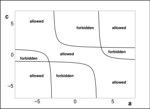
Figure 8: Boundaries $Q(a,b,c)=0$ and forbidden parts of the $a-c$ plane as sampled at $b^{2}=1$.

4.1 The auxiliary domains and their boundaries

The domain ${\cal D}^{(H)}$ of parameters for which our Hamiltonian $H^{(4)}(a,b,c)$ generates the unitary evolution of quantum system is defined as an intersection of the triplet of domains ${\cal D}^{(P,Q,W)}$ in $\mathbb{R}^{3}$. After the preparatory considerations as presented in the preceding sections let us now leave all of the three parameters $a$, $b$ and $c$ freely variable and recall that

• the domain ${\cal D}^{(P)}$ is defined by the inequality $P(a,b,c)=10-{a}^{2}-2\,{b}^{2}-{c}^{2}>0$. It is compact so that we may restrict our attention just to the intervals of $b^{2}<5$, $a^{2}<10$ and $c^{2}<10$. At any fixed $b^{2}<5$ the section of this first auxiliary domain coincides with the interior of a central circle in $a-c$ plane with radius $R=\sqrt{10-2b^{2}}$;

• the allowed interior of the triply connected domain ${\cal D}^{(Q)}$ is defined by the inequality $Q(a,b,c)=\left[(a+3)(c-1)-{b}^{2}\right]\left[(a-3)(c+1)-{b}^{2}\right]$. In the $a-c$ plane the boundaries of this domain are two hyperbolas sampled at $b^{2}=1$ in Fig.8;

• the third auxiliary domain ${\cal D}^{(W)}$ is defined by the inequality $W(a,b,c)=\left(8+c^{2}-a^{2}\right)^{2}-4\,\left[16-(a+c)^{2}\right]\,b^{2}>0$.

The description of the latter domain ${\cal D}^{(W)}$ is slightly less trivial. It may be based on the observation that the interior of this domain covers all the exterior of the strip where $|a+c|>4$. Then the interior of this strip may be reparametrized,

$$c-a=2\,\tau(c,a)\in(-\infty,\infty)\,,\ \ \ \ \ c+a=4\,\sin\varphi(c,a)\,,\ \ \ \varphi(c,a)\in(-\pi/2,\pi/2)\,$$

making the rest of the domain ${\cal D}^{(W)}$ determined by the elementary inequality

$$|b|<\frac{|1+\tau(c,a)\sin[\varphi(c,a)]|}{\cos[\varphi(c,a)]}\,.$$ (11)

This means that within the restricted range of $\tau(c,a)\in(-\sqrt{10},\sqrt{10})$ the growth of $|b|\to\infty$ must be compensated by the decrease of $\cos[\varphi(c,a)]\to 0$, i.e., by the convergence $c\to\pm 1-a$. This makes the strip-restricted part of the domain ${\cal D}^{(W)}$ very small but increasing with the decrease of $|b|$ from a sufficiently large initial value.

4.2 The boundaries of the cryptohermiticity domain

In the light of the latter comment it makes good sense to start the study of the “physical” overlaps ${\cal D}^{(W)}$ of the three auxiliary domains ${\cal D}^{(P,Q,W)}$ at the maximal admissible plane of $b=b^{(P)}=\sqrt{5}$ which touches the boundary $\partial{\cal D}^{(P)}$ at $a=c=0$. This points still lies out of the domains ${\cal D}^{(W)}$ and ${\cal D}^{(H)}$ since $W(0,\sqrt{5},0)=64-320<0$. In a search for the first touch between the $b-$plane and boundary $\partial{\cal D}^{(H)}$ we must diminish our $b$ and move into the interior of ${\cal D}^{(P)}$.

Figure 9: $b=\sqrt{5}-1/100=2.226067977$.

In the first illustrative example at $b=\sqrt{5}-1/100$ our Fig. 9 displays the motion of the triplet of boundaries $\partial{\cal D}^{(P,Q,W)}$ projected into the $a-c$ real plane. This picture shows that the corresponding section of the first domain ${\cal D}^{(P)}$ becomes nonempty. Still, it just occupies the interior of a very small circle $\mathbf{C}(b)=\partial{\cal D}^{(P)}|_{b=fixed}$ with the center at the origin.

Figure 10: $b=\sqrt{5}-1/2=1.736067977$.

The interior of the second domain ${\cal D}^{(Q)}$ is perceivably bigger since, in the manner indicated by Fig. 8 above, it occupies the large domain between the two outermost, $b-dependent$ hyperbolic curves $\mathbf{H}_{1,2}(b)\subset\partial{\cal D}^{(Q)}|_{b=fixed}$. The overlap ${\cal D}^{(H)}$ itself remains empty because the third domain ${\cal D}^{(W)}$ is localized behind the two remaining and less trivially parametrized curves $\mathbf{G}_{1,2}(b)\subset\partial{\cal D}^{(W)}|_{b=fixed}$.

Figure 11: $b=\sqrt{5}-1=1.236067977$.

During the subsequent decrease of $b$ sampled by Fig. 9 the two curves $\mathbf{G}_{j}(b)$ and $\mathbf{H}_{j}(b)$ (assigned the same subscript $j=1$ or $j=2$) get closer to each other while the internal circle $\mathbf{C}(b)$ gets larger. At each $j$ and at the same value of $b$ both the curves $\mathbf{G}_{j},\mathbf{H}_{j}$ touch the circle $\mathbf{C}(b)$. At a still smaller $b=\sqrt{5}-1/2=1.736067977$ they already move inside, sharing their two separate intersections with the circle. This situation is illustrated in Fig. 10.

Figure 12: $b=1.01$.

Figure 13: $b=1$.

At any $j$ and during the further decrease of the parameter $b$ the two triple-intersection points between $\mathbf{C}(b)$, $\mathbf{G}_{j}$ and $\mathbf{H}_{j}$ move apart. Between them one discovers the formation of the first two non-empty components of the physical domain ${\cal D}^{(H)}$. These components are disconnected, extremely narrow and eye-shaped, with the “eyes almost closed” but “slowly opening” with the further decrease of $b$. Graphically, the generic situation of this type in illustrated by Figs. 11 and 12.

Figure 14: $b=0.999$.

The next qualitative change of the pattern occurs at the above-mentioned special value of $b=1$ as which we touch the saddle of the surface $\partial{\cal D}^{(W)}$. Slightly before this happens we encounter the situation depicted in Fig. 12 where the two separate subdomains of the physical domain ${\cal D}^{(H)}|_{b=fixed}$ already almost touch. Next they do touch (cf. Fig. 13) and, subsequently, get connected (cf. the next Fig. 14).

Figure 15: $b=0.6$.

Surprisingly enough, below the saddle point $b=1$ the topological surprises are still not at the end. There are no real news even at $b=0.6$ (cf. Fig. 15). Nevertheless, in the latter picture we already must pay attention to the two subdomains with the maximal $a^{2}$s.

Figure 16: $b=0.4$.

Having selected just the right end of the (symmetric) picture at the positive $a\approx 3$ we reveal the emergence of a tendency towards a new intersection between the (up to now, safely external and non-interfering) second branches of the $Q(a,b,c,)-$related hyperbolas $\mathbf{H}_{j}^{(second)}$ and of the back-bending boundaries $\partial{\cal D}^{(W)}|_{b=fixed}$. For example, these curves get very close to each other but still do not intersect yet at $b=0.4$, staying also outside of the central circular domain ${\cal D}^{(P)}$ (cf. Fig. 16).

Figure 17: $b=0.2$.

The change of the pattern is finally achieved slightly below $b=0.4$, at the moment when both of the new intersection candidates touch the circle $\mathbf{C}(b)=\partial{\cal D}^{(P)}|_{b=fixed}$ in a single point. Subsequently, this point splits into the pair of the triple intersections and the further decrease of $|b|$ forms the pattern which is sampled in Fig. 17 at $b=0.2$ and in Fig. 18 at $b=0.1$.

Figure 18: A return to the triply connected ${\cal D}^{(H)}$ at $b=0.1$.

Figure 19: A magnified detail of Fig. 18.

Figure 20: A magnified detail of Fig. 19.

Certainly, the key features of the new situation are better visible, at the illustrative $b=0.1$, in its magnified presentation as mediated by Figs. 19 and 20). Now we may return to the limiting pattern of Fig. 4 where we witness the abrupt change of the topology caused by the final confluence of the straight and backbanding branch of the boundary $\partial{\cal D}^{(W)}|_{b=fixed}$ in the limit $b\to 0$.

Obviously, in a way confirmed by the complementary results of section 3.3 such a confluence of the boundaries only occurs in the limit so that the thee-dimensional version of the open set ${\cal D}^{(H)}$ is ultimately confirmed to be triply connected.

5 Summary

In the history of pure mathematics the specification of the horizons $\partial{\cal D}^{(H)}$ (called, often, “discriminant surfaces” in this context) has been perceived as a challenging and rather difficult problem even in its first “unsolvable” case characterized, in our present notation, by the Hilbert-space dimensions $N=5$ [11]. It is also certainly worth noticing that in certain mathematically natural directions the real progress is of an amazingly recent date [12]. In this connection it seems rather remarkable that certain parallel developments occured also in several applied-mathematics oriented studies paying attention to the natural presence of more symmetries in the Hamiltonian [7] and/or to the introduction of more observable quantities within a phenomenological quantum model in question [13].

In a constructive, more pragmatic setting as sampled by our recent paper [6] we restricted our attention to the topological aspects of the problem of horizons. The most obvious motivation of such an effort has been given by the fact that a disconnectedness of the domain ${\cal D}^{(H)}$ immediately requires the transition from its traditional perturbation-theory descriptions (with a recommended recent compact sample given in [14]) to non-perturbative methods, or to certain perturbative strong-coupling techniques at least [15]. In Ref. [6] the parallel and less formal motivation has been emphasized to lie in the systematic search for possible physical origin of the dynamical anomalies in a kinematical nontriviality of the topology of phase space.

The conclusions of our present paper are encouraging. Firstly we demonstrated that for many purposes it may be sufficient to use the matrices with a not too large $N$. Secondly, we have shown an increase of the feasibility of the description of models $H$ with certain additional symmetries. At the first nontrivial Hilbert-space dimension $N=4$ they reduced, for example, the minimal necessary number of parameters to $D=3$ or even to $D=2$ .

Thirdly we clarified that once one works with a tridiagonal-matrix form of the “unperturbed” $N$ by $N$ Hamiltonian $H^{(N)}_{0}$ complemented by certain computationally suitable specific perturbations, the existence of the disconnected subdomains in ${\cal D}^{(H)}$ opens the direct access to the strong-coupling dynamical regime.

Fourthly, on mathematical side, we are now able to recommend, strongly, the use of certain auxiliary symmetries in the Hamiltonians (e.g., the ones recommended in Ref. [16]). In such cases, the algebraic secular equations pertaining to the model often happen to factorize, leading to the much better tractable polynomial equations of perceivably lower orders.

Last but not least it seems worth emphasizing that even at our present “solvable” choice of the dimension $N=4$ the latter fact rendered our toy model more easily solvable. In fact, on the background given by Refs. [6, 17] it took some time for us to imagine that the anomalies of spectra could certainly start occurring at the very small dimensions $N<8$. In this context the message of our present $N=4$ study is encouraging. Partly because several specific spectral irregularities as observed at $N=8$ in Ref. [6] do also exist for certain very similar Hamiltonian matrices with the dimension as low as $N=4$, and partly because our model reconfirmed the hypothesis of a “hidden” topology-related connection between the loop-shaping of the lattices (i.e., presumably, Betti numbers in continuous limit) and the existence of definite strong-coupling dynamical anomalies in the spectra of the energy levels.

Appendix A. The three-Hilbert-space formulation of quantum mechanics

In section 2 of Ref. [5] one finds one of the most compact introductions into the abstract formalism of ${\cal PT}-$symmetric quantum mechanics (PTSQM). Thus, we may shorten here the introductory discussion and refrain ourselves to a few key comments on the general theoretical framework.

In such a compression the PTSQM formalism may be characterized as such a version of entirely standard quantum mechanics in which, in principle, the system in question is defined in a certain prohibitively complicated physical Hilbert space of states ${\cal H}^{(P)}$ where the superscript may be read as abbreviating “prohibited” as well as “physical” [3].

Typical illustrative realistic examples may be sought in the physics of heavy nuclei where the corresponding fermionic states are truly extremely complicated. In the latter exemplification the first half of the PTSQM recipe lies in the transition to a suitable, unitary equivalent Hilbert space, ${\cal H}^{(P)}\to{\cal H}^{(S)}$, where the superscript “^(S)” may stand for “suitable” or “simpler” [3].

In the above-mentioned realistic-system illustration, for example, the new space ${\cal H}^{(S)}$ coincided with a suitable “interacting boson model” (IBM). In the warmly recommended review paper of this field [18] it has been emphasized that the requirement of the unitary equivalence between the two Hilbert spaces ${\cal H}^{(P)}$ and ${\cal H}^{(S)}$ may only be achieved in two ways. Either the corresponding boson-fermion-like mapping $\Omega$ between these two Hilbert spaces (known, in this context, as the Dyson’s mapping) remains unitary (and the mathematical simplification of the problem remains inessential) or is admitted to be non-unitary (which is a less restrictive option which may enable us to achieve a really significant simplification, say, of the computational determination of the spectra).

What remains for us to perform and explain now is the second half of the general PTSQM recipe. Its essence lies in the weakening of the most common unitarity requirement imposed upon the Dyson’s mapping,

$$\Omega^{\dagger}=\Omega^{-1}$$

to the mere quasi-unitarity requirement

$$\Omega^{\dagger}=\Theta\,\Omega^{-1}\,.$$

The symbol $\Theta\neq I$ represents here the so called metric operator which defines the inner product in Hilbert space ${\cal H}^{(S)}$.

More details using the present notation may be found in [3]. Just a few of them have to be recalled here. Firstly, the main source of the purely technical simplifications of the efficient numerical calculations (say, of the spectra of energies) is to be seen in the introduction of the third, purely auxiliary Hilbert space ${\cal H}^{(F)}$ where the superscript “^(F)” combines the meaning of “friendlier” with “falsified” [3].

By definition, the two Hilbert spaces ${\cal H}^{(S)}$ and ${\cal H}^{(F)}$ coincide as the mathematical vector spaces (“of ket vectors” in the Dirac’s terminology). One only replaces the nontrivial metric $\Theta^{(S)}\ \equiv\ \Omega^{\dagger}\Omega$ of the former space by its trivial simplification $\Theta^{(F)}\ \equiv\ I$ in the latter Hilbert space. As an immediate consequence, the latter space acquires the status of an auxiliary, manifestly unphysical space which does not carry any immediate physical information or probabilistic interpretation of its trivial though, at the same time, maximally mathematically friendly inner products.

Appendix B. The role of ${\cal PT}-$symmetry

In its most widely accepted final form described in Ref. [1] the PTSQM recipe complements the latter general scheme by another assumption. It may be given the mathematical form of the introduction of the second auxiliary, manifestly unphysical vector space ${\cal K}^{({\cal P})}$ which is, by definition, not even the Hilbert space. In fact, this fourth vectors space is assumed endowed with the formal structure of the so called Krein space [19].

Ref. [14] may be consulted for more details. Here, let us only remind the readers that the symbol ${\cal P}$ in the superscript carries the double meaning and combines the mathematical role of the indefinite metric ${\cal P}$ (defining in fact the Krein space) with an input physical interpretation (usually, of the operator of parity). In addition, the theoretical pattern

$${\cal H}^{(S)}\leftrightarrow{\cal K}^{({\cal P})}\leftrightarrow{\cal H}^{(F)}\,.$$ (12)

gets complemented by the requirement that there exists a “charge” operator ${\cal C}$ such that the (by assumption, non-trivial, sophisticated) metric $\Theta^{(S)}\neq I$ which defines the inner product in the second Hilbert space ${\cal H}^{(S)}$ coincides with the product of the two above-mentioned operators,

$$\Theta^{(S)}={\cal PC}\,.$$ (13)

The contrast between the feasibility of the $N\neq 3$ constructions presented in Ref. [5] and the discouraging complexity and incompleteness of the next-step $N=4$ constructions as performed in our older paper [17] and in its sequels [7] was also thoroughly discussed in our review [8]. In our present text we do not deviate from the notation and conventions accepted of this review. We solely pay attention to the class of models where $N-$dimensional matrix of parity is unique and given, in advance, in the following form,

$${\cal P}=\left[\begin{array}[]{cccccc}1&0&\ldots&&\ldots&0\\ 0&-1&0&\ldots&\ldots&0\\ 0&0&1&0&\ldots&0\\ 0&0&0&-1&\ddots&\vdots\\ \vdots&\ddots&\ddots&\ddots&\ddots&0\\ 0&\ldots&0&0&0&\mp 1\end{array}\right]\,.$$ (14)

In parallel, we did make use of the time-reversal operator ${\cal T}$ of the form presented, e.g., in Ref. [5] as mediating just the transposition plus complex conjugation of vectors and/or matrices. One should add that once we solely work with real vectors and matrices, we are even allowed to perceive ${\cal T}$ as a mere transposition.

Acknowledgments

Work supported by the GAČR grant Nr. P203/11/1433, by the MŠMT “Doppler Institute” project Nr. LC06002 and by the Inst. Res. Plan AV0Z10480505.

References

- [1] Bender, C. M.: Making Sense of non-Hermitian Hamiltonians, Rep. Prog. Phys. Vol. 70 (2007), p. 947 - 1018 (arXiv: hep-th/0703096).
- [2] Dorey P., Dunning C., Tateo R.: The ODE/IM Correspondence, J. Phys. A: Math. Theor. Vol. 40 (2007) p. R205 - R283 (arXiv:hep-th/0703066); Davies, E. B.: Linear operators and their spectra, Cambridge, Cambridge University Press, 2007; Mostafazadeh A.: Pseudo-Hermitian Quantum Mechanics, arXiv:0810.5643.
- [3] Znojil, M.: Three-Hilbert-space formulation of Quantum Mechanics, SIGMA, Vol. 5 (2009), 001, 19 pages (arXiv:0901.0700).
- [4] Rüter, C. E., Makris, K. G., El-Ganainy, R., Christodoulides, D.N., Segev, M., Kip, D.: Observation of parity time symmetry in optics. Nat. Phys. Vol. 6 (2010), p. 192-195; Kottos, T.: Optical physics: Broken symmetry makes light work, Nat. Phys. Vol. 6 (2010), p. 166-167.
- [5] Wang, Q.-H., Chia, S.-Z., Zhang, J.-H., PT symmetry as a generalization of Hermiticity. J. Phys. A: Math. Theor. Vol. 43 (2010), p. 295301.
- [6] Znojil, M.: Anomalous real spectra of non-Hermitian quantum graphs in strong-coupling regime, J. Phys. A: Math. Theor. Vol. 43 (2010), p. 335303.
- [7] Znojil, M.: Tridiagonal PT-symmetric N by N Hamiltonians and a fine-tuning of their observability domains in the strongly non-Hermitian regime, J. Phys. A: Math. Theor. Vol. 40 (2007), 13131-13148; Znojil, M,: Conditional observability versus self-duality in a schematic model, J. Phys. A: Math. Theor. 41 (2008), p. 304027; Znojil, M.: A return to observability near exceptional points in a schematic PT-symmetric model, Phys. Lett. Vol. B 647 (2007), p. 225-230; Znojil, M.: Conditional observability, Phys. Lett. Vol. B 650 (2007), p. 440- 446.
- [8] Znojil, M.: PT-symmetric quantum chain models, Acta Polytechnica, Vol. 47 (2007), p. 9 - 14.
- [9] Znojil, M.: Novel recurrent approach to the generalized Su-Schrieffer-Heeger Hamiltonians, Phys. Rev. B Vol. 40 (1989), p. 12468-12475.
- [10] Znojil, M.: Horizons of stability, J. Phys. A: Math. Theor. Vol. 41 (2008), p. 244027.
- [11] Top, J., E. Weitenberg, E.: Models of discriminant surfaces, Bull. AMS Vol. 48 (2011), p. 85- 90.
- [12] Wagner, D. G.: Multivariate stable polynomials: theory and application, Bull. AMS Vol. 48 (2011), p. 53-84.
- [13] Znojil, M.: Coupled-channel version of PT-symmetric square well, J. Phys. A: Math. Gen. Vol. 39 (2006), p. 441 - 455.
- [14] Langer, H., Tretter, Ch.: A Krein space approach to PT-symmetry, Czech. J. Phys. Vol. 54 (2004), p. 1113.
- [15] Caliceti, E., Graffi, S., Maioli M.: Perturbation theory of odd anharmonic oscillators, Commun. Math. Phys. 75 (1980), p. 51-66; Fernández, F.M., Guardiola, R., Ros, J., Znojil, M.: Strong-coupling expansions for the PT-symmetric oscillators V(r) = a i x+ b (ix)2+ c(ix)3, J. Phys. A: Math. Gen. Vol. 31 (1998), p. 10105-10112.
- [16] Znojil, M.: Maximal couplings in PT-symmetric chain-models with the real spectrum of energies, J. Phys. A: Math. Theor. Vol. 40 (2007), p. 4863-4875.
- [17] Znojil, M.: Determination of the domain of the admissible matrix elements in the four-dimensional PT-symmetric anharmonic model, Phys. Lett. A Vol. 367 (2007), p. 300-306.
- [18] Scholtz, F. G., Geyer, H. B., Hahne, F. J. W.: Quasi-Hermitian Operators in Quantum Mechanics and the Variational Principle, Ann. Phys. Vol. 213 (1992), p. 74 - 101.
- [19] Nagy, K. L.: State Vector Spaces with Indefinite Metric in Quantum Field Theory, Budapest, Akademiai Kiado, 1966; Gohberg, I. C., Krein, M. G.: Introduction to the Theory of Linear Nonselfadjoint Operators, Providence, American Mathematical Society, 1969.