Combinatorics, observables, and String Theory

Andrea Gregori^†
Abstract
We investigate the most general phase space of configurations, consisting of all possible ways of assigning elementary attributes, “energies”, to elementary positions, “cells”. We discuss how this space possesses structures that can be approximated by a quantum-relativistic physical scenario. In particular, we discuss how the Heisenberg’s Uncertainty Principle and a universe with a three-dimensional space arise, and what kind of mechanics rules it. String Theory shows up as a complete representation of this structure in terms of time-dependent fields and particles. Within this context, owing to the uniqueness of the underlying mathematical structure it represents, one can also prove the uniqueness of string theory.

 ^†e-mail: agregori@libero.it

1 Introduction

The search for a unified description of quantum mechanics and general relativity, within a theory that should possibly describe also the evolution of the universe, is one of the long standing and debated open problems of modern theoretical physics. The hope is that, once such a theory has been found, it will open us a new perspective from which to approach, if not really answer, the fundamental question behind all that, that is “why the universe is what it is”. On the other hand, it is not automatical that, once such a unified theory has been found, it gives us also more insight on the reasons why the theory is what it is, namely, why it has to be precisely that one, and why no other choice could work. But perhaps it is precisely going first through this question that it is possible to make progress in trying to solve the starting problem, namely the one of unifying quantum mechanics and relativity. Indeed, after all we don’t know why do we need quantum mechanics, and relativity, or, equivalently, why the speed of light is a universal constant, or why there is the Heisenberg Uncertainty. We simply know that, in a certain regime, Quantum Mechanics and Relativity work well in describing physical phenomena.

In this work, we approach the problem from a different perspective. The question we start with can be formulated as follows: is it possible that the physical world, as we see it, doesn’t proceed from a “selection” principle, whatever this can be, but it is just the collection of all the possible “configurations”, intended in the most general meaning? May the history of the Universe be viewed somehow as a path through these configurations, and what we call time ordering an ordering through the inclusion of sets, so that the universe at a certain time is characterized by its containing as subsets all previous configurations, whereas configurations which are not contained belong to the future of the Universe? What is the meaning of “configuration”, and how are then characterized configurations, in order to say which one is contained and which not? How do they contribute to make up what we observe?

Let us consider the most general possible phase space of “spaces of codes of information”. By this we mean products of spaces carrying strings of information of the type “1” or “0”. If we interpret these as occupation numbers for cells that may bear or not a unit of energy, we can view the set of these codes as the set of assignments of a map $\Psi$ from a space of unit energy cells to a discrete target vector space, that can be of any dimensionality. If we appropriately introduce units of length and energy, we may ask what is the geometry of any of these spaces. Once provided with this interpretation, it is clear that the problem of classifying all possible information codes can be viewed as a classification of the possible geometries of space, of any possible dimension. If we consider the set of all these spaces, i.e. the set of all maps, $\left\{\Psi\right\}$, that we call the phase space of all maps, we may also ask whether some geometries occur more or less often in this phase space. In particular, we may ask this question about $\left\{\Psi(E)\right\}$, the set of all maps which assign a finite amount of energy units, $N\equiv E$. The frequency by which these spaces occur depends on the combinatorics of the energy assignments . Indeed, it turns out that not only there are configurations which occur more often than other ones, but that there are no two configurations with the same weight. If we call $\left\{\Psi(E)\right\}$ the “universe” at “energy” $E$, we can see that we can assign a time ordering in a natural way, because $\left\{\Psi(E^{\prime})\right\}$ “contains” $\left\{\Psi(E)\right\}$ if $E^{\prime}>E$, in the sense that $\forall\Psi\in\left\{\Psi(E)\right\}$ $\exists\Psi^{\prime}\in\left\{\Psi(E^{\prime})\right\}$ such that $\Psi\subsetneqq\Psi^{\prime}$. $E$ plays therefore the role of a time parameter, that we can call the age of the universe, ${\cal T}$. Our fundamental assumption is that, at any time $E$, there is no “selected” geometry of the universe: the universe as it appears is given by the superposition of all possible geometries. Namely, we assume that the partition function of the universe, i.e. the function through which all observables are computed, is given by:

$${\cal Z}(E)\,=\,\sum_{\Psi(E)}{\rm e}^{S(\Psi(E))}\,,$$ (1.1)

where $S(\Psi)$ is the entropy of the configuration $\Psi$ in the phase space $\left\{\Psi\right\}$, related to the weight of occupation in the phase space $W(\Psi)$ in the usual way: $S=\log W$. Rather evidently, the sum is dominated by the configurations of highest entropy.

The most recurrent geometries of this universe turn out to be those corresponding to three dimensions. Not only, but the very dominant configuration is the one corresponding to a three-sphere of radius $R$ proportional to $E$. That is, a black hole-like universe in which the energy density is $\sim 1/E^{2}\propto 1/R^{2}$ . But the most striking feature is that all the other configurations summed up contribute for a correction to the total energy of the universe of the order of $\Delta E\sim 1/{\cal T}$. This is rather reminiscent of the inequality at the base of the Heisenberg Uncertainty Principle on which quantum mechanics is based on: ${\cal T}$, the age/radius up to the horizon of observation, can also be written as $\Delta t$, the interval of time during which the universe of radius $E$ has been produced. That means, the universe is mostly a classical space, plus a “smearing” that quantitatively corresponds to the Heisenberg Uncertainty, $\Delta E\sim 1/\Delta t$. This argument can be refined and applied to any observable one may define: all what we observe is given by a superposition of configurations and whatever value of observable quantity we can measure is smeared around, is given with a certain fuzziness, which corresponds to the Heisenberg’s inequality. Indeed, a more detailed inspection of the geometries that arise in this scenario, the way “energy clusters” arise, their possible interpretation in terms of matter, particles etc. allows to conclude that 1.1 formally implies a quantum scenario, in which the Heisenberg Uncertainty receives a new interpretation. The Heisenberg uncertainty relation arises here as a way of accounting not simply for our ignorance about the observables, but for the ill-definedness of these quantities in themselves: all the observables that we may refer to a three-dimensional world, together with the three-dimensional space itself, exist only as “large scale” effects. Beyond a certain degree of accuracy they can neither be measured nor be defined. The space itself, with a well defined dimension and geometry, cannot be defined beyond a certain degree of accuracy either. This is due to the fact that the universe is not just given by one configuration, the dominant one, but by the superposition of all possible configurations, an infinite number, among which many (an infinite number) don’t even correspond to a three dimensional geometry. The physical reality is the superposition all possible configurations, weighted as in 1.1.

It is also possible to show that the speed of expansion of the geometry of the dominant configuration of the universe, i.e. the speed of expansion of the radius of the three-dimensional black hole, that by convention and choice of units we can call “$c$”, is also the maximal speed of propagation of coherent, i.e. non-dispersive, information. This can be shown to correspond to the $v=c$ bound of the speed of light. Here it is essential that we are talking of coherent information, as tachyonic configurations also exist and contribute to 1.1: their contribution is collected under the Heisenberg uncertainty.

One may also show that the geometry of geodesics in this space corresponds to the one generated by the energy distribution. This means that this framework “embeds” in itself Special and General Relativity.

The dynamics implied by (1.1) is neither deterministic in the ordinary sense of causal evolution, nor probabilistic. At any age the universe is the superposition of all possible configurations, weighted by their “combinatorial” entropy in the phase space. According to our definition of time and time ordering, at any time the actual superposition of configurations does not depend on the superposition at a previous time, because the actual and the previous one trivially are the superposition of all the possible configurations at their time. Nevertheless, on the large scale the flow of mean values through time can be approximated by a smooth evolution that we can, up to a certain extent, parametrize through evolution equations. As it is not possible to exactly perform the sum of infinite terms of 1.1, and it does not even make sense, because an infinite number of less entropic configurations don’t even correspond to a description of the world in terms of three dimensions, it turns out to be convenient to accept for practical purposes a certain amount of unpredictability, introduce probability amplitudes and work in terms of the rules of quantum mechanics. These appear as precisely tuned to embed the uncertainty that we formally identified with the Heisenberg Uncertainty into a viable framework, which allows some control of the unknown, by endowing the uncertainty with a probabilistic interpretation. Within this theoretical framework, we can therefore give an argument for the necessity of a quantum description of the world: quantization appears to be a useful way of parametrizing the fact of being the observed reality a superposition of an infinite number of configurations. Once endowed with this interpretation, this scenario provides us with a theoretical framework that unifies quantum mechanics and relativity in a description that, basically, is neither of them: in this perspective, they turn out to be only approximations, valid in a certain limit, of a more comprehensive formulation.

The scenario implied by 2.35 is highly predictive, in that there is basically no free parameter, except for the only running quantity, the age of the universe, in terms of which everything is computed. Out of the dominant configuration, a three-sphere, the contribution given by the other configurations to (1.1) is responsible for the introduction of “inhomogeneities” in the universe. These are what gives rise to a varied spectrum of energy clusters, that we interpret as matter and fields evolving and interacting during a time evolution set by the $E$–time-ordering. All of them fall within the corrections to the dominant geometry implied by the Heisenberg’s inequality. For instance, matter clusters constitute local deviations of the mean energy/curvature of order $\Delta E\sim 1/\Delta t$, where $\Delta t$ is the typical time extension (or, appropriately converted through the speed of light, the space extension) of the cluster, and so on.

In this framework, String Theory arises as a consistent quantum theory of gravity and interacting fields and particles, which constitutes a useful mapping of the combinatorial problem of “distribution of energy along a target space” into a continuum space. To this purpose, one must think at string theory as defined in an always compact, although arbitrarily extended, space. By “String Theory” we mean here the collection of all supersymmetric string constructions, which are supposed to be particular realizations of a unique theory underlying all the different string constructions. In this sense, when we speak of a string configuration, this has to be intended as a (generally non-perturbative) configuration of which the possible perturbative constructions made in terms of heterotic, type II, type I string, represent “slices”, dual aspects of the same object. Owing to quantization, and therefore to the embedding of the Heisenberg’s Uncertainties, the space of all possible string configurations “covers” all the cases of the combinatorial formulation, of which it provides a representation in terms of a probabilistic scenario, useful for practical computations. Indeed, in this theoretical framework precisely the “uniqueness” of the combinatorial scenario (because of its being absolutely general), and the fact of being the collection of string constructions a faithful and complete representation in terms of fields and particles of this absolutely general structure, allow to view in a different light the problem of the “uniqueness of string theory”, namely the fact that all perturbative superstring constructions should be part of a unique theory.

In order to be a representation of the combinatorial scenario, as it happens for the universe coming out of the geometry of codes, also the physical string vacuum must not follow a selection rule. In correspondence to the phase space of all the energy-combinatorial configurations, it is possible to introduce the phase space of all string configurations, and the corresponding partition function for the universe at any age. Since we work on the continuum, instead of a sum the partition function of the string phase space will be an integral:

$${\cal Z}_{\rm string}\,=\,\int{\cal D}\psi\,{\rm e}^{S(\psi)}\,.$$ (1.2)

One can show that, in order to correctly reproduce the conditions of the combinatorial problem, the ordering must be taken through the degree of symmetry and the volume of the compact space these configurations are based on.

The detailed analysis of the string configuration of highest entropy and the corresponding spectrum of particles and fields will be discussed in Ref. [1](see also [2]), together with a discussion of various cosmological bounds (Oklo bound, nucleosynthesis bound), etc. In this paper we discuss the theoretical grounds of this approach, revisiting and completing the content of Refs. [3] and [4]. As in Ref. [3], we start our analysis in section 2 by investigating the combinatorics of the “distribution of binary attributes”, and discuss how, and in which sense, certain structures dominate. This allows to see an “order” in this “darkness”. We discuss how a “geometry” shows up, and how geometric inhomogeneities, that we can interpret as the discrete version of “wave packets”, arise. We recover in this way, through a completely different approach, all the known concepts of particles and masses. In the “phase space” constituted by all possible configurations we introduce the “time ordering” based on the inclusion of configurations, and discuss what is the dimension and geometry which is statistically dominant. In section 3 we discuss how the Uncertainty Principle shows up in this framework, and what is its interpretation. We devote section 4 to a discussion of the issues of causality and in what limit “quantum mechanics” arises in this framework. In section 5 we draw on the arguments of Ref. [4] to discuss how this scenario implies also Relativity.

We pass then (section 6) to discuss what is the role played by string theory in this scenario: in which sense and up to what extent it provides an approximation to the description of the combinatoric/geometric scenario, of which Quantum (Super) String Theory constitutes an implementation in the framework of a continuum (differentiable) space. String Theory is consistent only in a finite number of dimensions. Therefore, it would seem that it represents only a subset of the configurations of the combinatorial approach, a subspace of the full phase space. However, through the implementation of quantization, and therefore of the Heisenberg’s Uncertainty Principle, it considers also the neglected configurations of the phase space, covering them under the uncertainty which is “built in” in its basic definition. In other words, it comes already endowed with a “fuzziness” that incorporates in its range the contribution of all the other possible configurations. It is precisely due to this completeness, ensured by canonical quantization, that String Theory can be seen to constitute a unique theory, of which the various perturbative constructions constitute dual slices. Canonical quantization can be also shown to be directly related to the dimensionality of space-time; it is precisely upon quantization that string theory is forced to a critical dimension, which implies as most entropic compactification a configuration with four space-time dimensions. At the end of the section we discuss then how the integral 1.2 can be viewed as the analogous of the Feynman path integral for string configurations. This supports the idea that 1.1 constitutes the natural extension of quantum field theory to gravity. The concept of “weighted sum over all paths” is substituted by a weighted sum over all energy/space configurations. The traditional question about “how to find the right string vacuum” is then surpassed in a way that looks very natural for a quantum scenario: the concept of “right solution” is a classical concept, as is the idea of “trajectory”, compared to the path integral. The physical configuration takes all the possibilities into account. As much as the usual path integral contains all the quantum corrections to a classical trajectory, similarly here in the functional 1.1 the sum over all configurations accounts for the corrections to the classical, geometric vacuum.

In section 7 we discuss how the Universe, as it appears to an observer, builds up. In particular, we discuss what is the meaning of boundary and horizon in such a spheric geometry, and how an understanding of these properties is only possible outside of the domain, and the properties, of classical geometry: all oddities and paradoxes find their explanation only within what we call quantum geometry. We conclude with some comments about how fundamental is a description of the world in terms of discrete (binary) codes. We argue that real numbers (the continuum) doesn’t add any information to a description made in terms of binary codes, which therefore seems to be the most fundamental description of nature. But our investigation, and the approach we are proposing, leads us to dare asking another question, about what is after all the world we experience. We are used to order our observations according to phenomena that take place in what we call space-time. An experiment, or, better, an observation (through an experiment), basically consists in realizing that something has changed: our “eyes” have been affected by something, that we call “light”, that has changed their configuration (molecular, atomic configuration). This light may carry information about changes in our environment, that we refer either to gravitational phenomena, or to electromagnetic ones, and so on… In order to explain them we introduce energies, momenta, “forces”, i.e. interactions, and therefore we speak in terms of masses, couplings etc… However, all in all, what all these concepts refer to is a change in the “geometry” of our environment, a change that “propagates” to us, and eventually results in a change in our brain, the “observer”. But what is after all geometry, other than a way of saying that, by moving along a path in space, we will encounter or not some modifications? Assigning a “geometry” is a way of parametrizing modifications. Is it possible then to invert the logical ordering from reality to its description? Namely, can we argue that what we interpret as energy, or geometry, is simply a code of information? Something happens, i.e. time passes, when the combinatorial of possible codes changes. Viewed in this way, it is not a matter of mapping physical degrees of freedom to a language of abstract codes, but the other way around, namely: perhaps the deepest reality is “information”, that we arrange in terms of geometries, energies, particles, fields, and interactions. Consider the most general and generic code. At the end of this paper, we argue that any code can be expressed as a binary code. In this new point of view, the universe is the collection of all possible codes. In order to “see” the universe, we must interpret these codes in terms of maps, from a space of “energies” to a target space, that take the “shape” of what we observe as the physical reality. From this point of view, information is not just something that transmits knowledge about what exists, but it is itself the essence of what exists, and the rationale of the universe is precisely that it ultimately is the whole of rationale.

For a detailed analysis of the spectrum of the theory implied by 1.1 and 1.2, and the phenomenological implications, we refer the reader to [1], [5] [6], and [7]. In particular, Refs. [5] and [7] show how this theoretical framework, being on its ground a new approach to quantum mechanics and phenomenology, does not simply provide us with possible answers to problems which are traditionally referred to quantum gravity and string theory, but opens new perspectives about problems apparently pertaining to other domains of physics, such as (high temperature) superconductivity and evolutionary biology.

2 The general set up

Consider the system constituted by the following two ”cells”:

(2.3)

Let’s assume that the only degrees of freedom this system possesses are that each one of the two cells can independently be white or black. We have the following possible configurations:

(2.4)

(2.5)

(2.6)

(2.7)

This is the “phase space” of our system. The configuration “one cell white, one cell black” is realized two times, while the configuration “two cells white” and “two cells black” are realized each one just once. Let’s now abstract from the practical fact that these pictures appear inserted in a page, in which the presence of a written text clearly selects an orientation. When considered as a “universe”, something standing alone in its own, configuration 2.5 and 2.6 are equivalent. In the average, for an observer possessing the same “symmetry” of this system (we will come back later to the subtleties of the presence of an observer), the “universe” will appear something like the following:

(2.8)

or, equivalently, the following:

(2.9)

namely, the “sum”:

(2.10)

or equivalently the sum:

(2.11)

Notice that the observer “doesn’t know” that we have rotated the second and third term, because he possesses the same symmetries of the system, and therefore is not able to distinguish the two cases by comparing the orientation with, say, the orientation of the characters of the text. What he sees, is a universe consisting of two cells which appear slightly differentiated, one “light gray”, the other “dark gray”.

The system just described can be viewed as a two-dimensional space, in which one coordinate specifies the position of a cell along the “space”, and the other coordinate the attribute of each position, namely, the color. Our two-dimensional “phase space” is made by $2({\rm space})\times 2({\rm colors})$ cells. By definition the volume occupied in the phase space by each configuration (two white; two black; one white one black) is proportional to the logarithm of its entropy. The highest occupation corresponds to the configuration with highest entropy. The effective appearance, one light-gray one dark-gray, 2.8 or 2.9, mostly resembles the highest entropy configuration.

Let’s now consider in general cells and colors. The colors are attributes we can assign to the cells, which represent the positions in our space. On the other hand, these “degrees of freedom” can themselves be viewed as coordinates. Indeed, if in our space with $m({\rm space})\times n({\rm colors})$ we have $n>m$, then we have more degrees of freedom than places to allocate them. In this case, it is more appropriate to invert the interpretation, and speak of $n$ places to which to assign the $m$ cells. The colors become the space and the cells their “attributes”. Therefore, in the following we consider always $n\leq m$.

2.1 Distributing degrees of freedom

Consider now a generic “multi-dimensional” space, consisting of $M_{1}^{p_{1}}\times\ldots\times M_{i}^{p_{i}}\ldots\times M_{n}^{p_{n}}$ “elementary cells”. Since an elementary, “unit” cell is basically a-dimensional, it makes sense to measure the volume of this $p$-dimensional space, $p=\sum^{n}_{i}p_{i}$, in terms of unit cells: $V=M_{1}^{p_{i}}\times\ldots\times M_{n}^{p_{n}}\stackrel{{\scriptstyle\rm def}}{{\equiv}}M^{p}$. Although with the same volume, from the point of view of the combinatorics of cells and attributes this space is deeply different from a one-dimensional space with $M^{p}$ cells. However, independently on the dimensionality, to such a space we can in any case assign, in the sense of “distribute”, $N\leq M^{p}$ “elementary” attributes. Indeed, in order to preserve the basic interpretation of the “$N$” coordinate as “attributes” and the “$M$” degrees of freedom as “space” coordinates, to which attributes are assigned, it is necessary that $N\leq M_{n}$, $\forall\,n$ . What are these attributes? Cells, simply cells: our space doesn’t know about “colors”, it is simply a mathematical structure of cells, and cells that we attribute in certain positions to cells. By doing so, we are constructing a discrete “function” $y=f(\vec{x})$, where $y$ runs in the “attributes” and $\vec{x}\in\{M^{\otimes p}\}$ belongs to our $p$-dimensional space. We define the phase space as the space of the assignments, the “maps”:

$$N\,\to\,\prod_{i}\otimes M_{i}^{\otimes p_{i}}\,,~{}~{}~{}~{}~{}M_{i}\,\geq\,N\,.$$ (2.12)

For large $M_{i}$ and $N$, we can approximate the discrete degrees of freedom with continuous coordinates: $M_{i}\to r_{i}$, $N\to R$. We have therefore a $p$-dimensional space with volume $\prod r_{i}^{p_{i}}$, and a continuous map $\vec{x}\in\{\vec{r}^{\vec{p}}\}\stackrel{{\scriptstyle f}}{{\to}}y\in\{R\}$, where $y$ spans the space up to $R=\prod r_{i}^{p_{i}}\equiv r^{p}$ and no more. In the following we will always consider $M_{i}\gg N$, while keeping $V=M^{p}$ finite. This has to considered as a regularization condition, to be eventually relaxed by letting $V\to\infty$.

An important observation is that there do not exist two configurations with the same entropy: if they have the same entropy, they are perceived as the same configuration. The reason is that we have a combinatoric problem, and, at fixed $N$, the volume of occupation in the phase space is related to the symmetry group of the configuration. In practice, we classify configurations through combinatorics: a configuration corresponds to a certain combinatoric group. Now, discrete groups with the same volume, i.e. the same number of elements, are homeomorphic. This means that they describe the same configuration. Configurations and entropies are therefore in bijection with discrete groups, and this removes the degeneracy. Different entropy = different occupation volume = different volume of the symmetry group; in practice this means that we have a different configuration.

We ask now: what is the most realized configuration, namely, are there special combinatorics in such a phase space that single out “preferred” structures, in the same sense as in our “two-cells $\times$ two colors” example we found that the system in the average appears “light-gray–dark-gray”? The most entropic configurations are the “maximally symmetric” ones, i.e. those that look like spheres in the above sense.

2.2 Entropy of spheres

Let us now consider distributing the $N$ energy attributes along a $p$-sphere of radius $m$. We ask what are the most entropic ways of occupy $N$ of the $\sim m^{p}$ cells of the sphere . For any dimension, the most symmetric configuration is of course the one in which one fulfills the volume, i.e. $N\sim m^{p}$. However, we are bound to the constraint $N\leq m$ for any coordinate, otherwise we loose the interpretation at the ground of the whole construction, namely of $N$ as the coordinate of attributes, and $m$ as the target of the assignment. $N\sim m^{p}$ means $m\sim\sqrt[p]{N}$, which implies $m<N$. The highest entropy we can attain is therefore obtained with the largest possible value of $N$ as compared to $m$, i.e. $N=m$, where once again the equality is intended up to an appropriate, $p$-dependent coefficient. Let us start by considering the entropy of a three-sphere. The weight in the phase space will be given by the number of times such a sphere can be formed by moving along the symmetries of its geometry, times the number of choices of the position of, say, its center, in the whole space. Since we eventually are going to take the limit $V\to\infty$, we don’t consider here this second contribution, which is going to produce an infinite factor, equal for each kind of geometry, for any finite amount of total energy $N$. We will therefore concentrate here on the first contribution, the one that from three-sphere and other geometries. To this purpose, we solve the “differential equation” (more properly, a finite difference equation) of the increase in the combinatoric when passing from $m$ to $m+1$. Owing to the multiplicative structure of the phase space (composition of probabilities), expanding by one unit the radius, or equivalently the scale of all the coordinates, means that we add to the possibilities to form the configuration for any dimension of the sphere some more $\sim m+1$ times (that we can also approximate with $m$, because we work at large $m$) the probability of one cell times the weight of the configuration of the remaining $m$ (respectively $m-1$) cells. But this is not all the story: since distributing $N$ energy cells along a volume scaling as $\sim m^{3}$, $m\geq N$ means that our distribution does not fulfill the space, the actual symmetry group of the distribution will be a subgroup of the whole group of the pure ”geometric” symmetry: moving along this space by an amount of space shorter than the distance between cells occupied by an energy unit will not be a symmetry, because one moves to a ”hole” of energy. It is easy to realize that in such a ”sparse” space, the effective symmetry group will have a volume that stays to the volume of a fulfilled space in the same ratio as the respective energy densities. Taking into account all these effects, we obtain the following scaling:

$$W(m+1)_{3}\,\sim\,W(m)_{3}\times(m+1)^{3}\times{N\over m^{3}}\times{m\over N}\,.$$ (2.13)

The last factor expresses the density of a circle, whereas the factor ${N\over m^{3}}$ is the density of the three-sphere. In order to make the origin of the various terms more clear, in these expressions we did not use explicitly the fact that actually $N$ is going to be eventually identified with $m$. Indeed, in 2.13 there should be one more factor: when we pass from radius $m$ to $m+1$ while keeping $N$ fixed, the configuration becomes less dense, and we loose a symmetry factor of the order of the ratio of the two densities: $[m/(m+1)]^{3}\sim 1+{\cal O}(1/m)$. Expanding $W(m+1)$ on the left hand side of 2.13 as $W(m)\,+\,\Delta W(m)$, and neglecting on the r.h.s. corrections of order $1/m$, we can write it as:

$${\Delta W(m)_{3}\over W(m)_{3}}\,\simeq\,m\,.$$ (2.14)

Since we are interested in the behavior at large $m$, we can approximate it with a continuous variable, $m\to x$, $x$, and approximate the finite difference equation with a differential one. Upon integration, we obtain:

$$S_{3}\,\propto\,\ln W(m)_{3}\,\sim\,{1\over 2}\,m^{2}\,,$$ (2.15)

where it is intended that $N=m$. Without this identification, the factor $(m/N)$ in 2.13 would not be the density of a 1-sphere. Under this condition, the energy density of the three-sphere scales as $1/N^{2}$, and we obtain an equivalence between energy density and curvature $R$:

$$\rho_{3}(N)\,\sim\,{1\over N^{2}}~{}\cong~{}{1\over r^{2}}\,\sim\,R_{(3)}\,.$$ (2.16)

This is basically the Einstein’s equation relating the curvature of space to the tensor expressing the energy density. Indeed, here this relation can be assumed to be the physical description of a sphere in three dimension. We can certainly think to formally distribute the $N$ energy units along any kind of space with any kind of geometry, but what makes a curved space physically distinguishable from a flat one, and a particular geometry from another one? Geometries are characterized by the curvature, but how does one observer measure the curvature? The coordinates $m$ of the target space have no meaning without energy units distributed along them. The geometry is decided by the way we assign the $N$ occupation positions. Here therefore we assume that measuring the curvature of space is nothing else than measuring the energy density. For the time being, let us just take the equivalence between energy density and curvature as purely formal; we will see in the next sections that this, with our definition of energy, will also imply that physical particles move along geodesics of the so characterized space, precisely as one expects from the Einstein’s equations. We will come back to these issues in section 5. In a generic dimension $p\geq 2$ the condition for having the geometry of a sphere reads :

$$\rho_{p}(E)\,\sim\,{N\over m^{p}}~{}\cong~{}{1\over m^{2}}\,.$$ (2.17)

In dimension $p\geq 3$ it is solved by:

$$m\,\sim\,N^{1\over p-2}~{}<\,N\,,~{}~{}~{}p\geq 3\,.$$ (2.18)

In two dimensions, 2.17 implies $N=1$ (up to some numerical coefficient). This means that, although it is technically possible to distribute $N>1$ energy units along a two-sphere of radius $m>1$, from a physical point of view these configurations do not describe a sphere. This may sound strange, because we can think about a huge number of spheric surfaces existing in our physical world, and therefore we may have the impression that attempting to give a characterization of the physical world in the way we are here doing already fails in this simple case. The point is that all the two spheres of our physical experience do not exist as two-dimensional spaces alone, but only as embedded in a three-dimensional physical space. i.e. as subspaces of a three-dimensional space. In dimensions higher than three, the equivalent of 2.13 reads:

$$W(m+1)_{p}\,\sim\,W(m)_{p}\times(m+1)^{p}\times{N\over m^{p}}\times{m\over N}\,.$$ (2.19)

The last term on the r.h.s. is actually one, because it was only formally written as $N/m$ to keep trace of the origin of the various terms. Indeed, it indicates the density of a fulfilling space, to which the scaling of the weight of any dimension must be normalized. Inserting the condition for the $p$-sphere, equation 2.17, we obtain:

$$W(m+1)_{p}\,\sim\,W(m)_{p}\times(m+1)^{p}\times{1\over m^{2}}\,,$$ (2.20)

which leads to the following finite difference equation:

$${\Delta W(m)_{p}\over W(m)_{p}}~{}\approx~{}m^{p-2}\,.$$ (2.21)

This expression obviously reduces to 2.14 for $p=3$. Proceeding as before, by transforming the finite difference equation into a differential one, and integrating, we obtain:

$$S_{(p\geq 2)}\,\propto\,\ln W(m)\,\sim\,{1\over p-1}\,m^{p-1}\,,~{}~{}~{}~{}p\geq 3\,.$$ (2.22)

This is the typical scaling law of the entropy of a $p$-dimensional black hole (see for instance [8]). For $p=2$, if we start from 2.19, without imposing the condition 2.17 of the sphere, we obtain, upon integration:

$$S_{(2)}\,\sim\,N^{2}\,,$$ (2.23)

formally equivalent to the entropy of a sphere in three dimensions. However, the fact that the condition of the sphere 2.17 implies $N=1$ means that a homogeneous distribution of the $N$ energy units corresponds to a staple of $N$ two-spheres. Indeed, if we use 2.20 and 2.21, for which the condition $N=1$ is intended, we obtain:

$$S_{(2)}\,\sim\,m\,.$$ (2.24)

For a radius $m=N$, this gives $1/N$ of the result 2.23, confirming the interpretation of this space as the superposition of $N$ spheres. From a physical point of view, we have therefore $N$ times the repetition of the same space, whose true entropy is not $N^{2}$ but simply $N$. As we will see in the next sections, such a kind of geometries correspond to what we will interpret as quantum corrections to the geometry of the universe. In the case of $p=1$, from a purely formal point of view the condition of the sphere 2.17 would imply $N=1/m$. Inserted in 2.19 and integrated as before, it gives:

$$S_{(1)}\,\propto\,\ln W(m)\,\sim\,\ln m\,,~{}~{}~{}~{}~{}~{}p=1\,.$$ (2.25)

Indeed, in the case of the one-sphere, i.e. the circle, one does not speak of Riemann curvature, proportional to $1/r^{2}$, but simply of inverse of the radius of curvature, $1/r$. It is on the other hand clear that the most entropic configuration of the one-dimensional space is obtained by a complete fulfilling of space with energy units, $N=m$, and that the weight in the phase space of this configuration is simply:

$$W(N)_{1}\,\sim\,N\,,$$ (2.26)

in agreement with 2.25 . For the spheres in higher dimension, from expression 2.22 and 2.18we derive:

$$S_{(p\geq 3)}|_{N}\,\sim\,{1\over p-1}\,m^{p-1}\,\sim\,{1\over p-1}\,N^{p-1\over p-2}\,.$$ (2.27)

For large $p$ the weights tend therefore to a $p$-independent value:

$$W(N)_{p}~{}\stackrel{{\scriptstyle p\ggg 3}}{{\longrightarrow}}~{}\approx\,{\rm e}^{N}\,,$$ (2.28)

and their ratios tend to a constant. As a function of $N$ they are exponentially suppressed as compared to the three-dimensional sphere. The scaling of the effective entropy as a function of $N$ allows us to conclude that:

• At any energy $N$, the most entropic configuration is the one corresponding to the geo-

  metry of a three-sphere. Its relative entropy scales as $S\sim N^{2}$.

Spheres in different dimension have an unfavored ratio entropy/energy. Three dimensions are then statistically “selected out” as the dominant space dimensionality.

2.3 The “time” ordering

Consider the set $\Phi(N)\equiv\{\Psi(N)\}$ of all configurations at any dimensionality $p$ and volume $V\gg N$ ($V\to\infty$ at fixed $N$). A property of $\Phi(N)$ is that, if $M<N$ $\forall\Psi(M)\in\Phi(M)$ $\exists\Psi^{\prime}(N)\in\Phi(M)$ such that $\Psi^{\prime}(N)\supsetneq\Psi(M)$, something that, with an abuse of language, we write as: $\Phi(N)\supset\Phi(M)$, $\forall~{}M<N$. It is therefore natural to introduce now an ordering in the whole phase space, that we call a “time-ordering”, through the identification of $N$ with the time coordinate: $N\leftrightarrow t$. We call “history of the Universe” the “path” $N\to\Phi(N)$ . This ordering turns out to quite naturally correspond to our every day concept of time ordering. In our normal experience, the reason why we perceive a history basically consisting in a progress toward increasing time lies on the fact that higher times bear the “memory” of the past, lower times. The opposite is not true, because “future” configurations are not contained in those at lower, i.e. earlier, times. But in order to be able to say that an event $B$ is the follow up of $A$, $A\neq B$ (time flow from $A\to B$), at the time we observe $B$ we need to also know $A$. This precisely means $A\in\Phi(N_{A})$ and $A\in\Phi(N_{B})$, which implies $\Phi(N_{A})\subset\Phi(N_{B})$ in the sense we specified above. Time reversal is not a symmetry of the system .

2.4 How do inhomogeneities arise

We have seen that the dominant geometry, the spheric geometry, corresponds to a homogeneous distribution of cells along the positions of the space, that we illustrate in figure 2.29,

(2.29)

where we mark in black the occupied cells. However, also the following configurations have spheric symmetry:

                       (2.30)

They are obtained from the previous one by shifting clockwise by one position the occupied cell. One would think that they should sum up to an apparent averaged distribution like the following:

(2.31)

This is not true: the Universe will indeed look like in figure 2.31, however this will be the “smeared out” result of the configuration 2.29. As long as there are no reference points in the space, which is an absolute space, all the above configurations are indeed the same configuration, because nobody can tell in which sense a configuration differs from the other one: “shifted clockwise” or “counterclockwise” with respect to what? We will discuss later how the presence of an observer by definition breaks some symmetries. Let’s see here how inhomogeneities (and therefore also configurations that we call “observers”) do arise. Configurations with almost maximal, although non-maximal entropy, correspond to a slight breaking of the homogeneity of space. For instance, the following configuration, in which only one cell is shifted in position, while all the other ones remain as in 2.29:

(2.32)

This configuration will have a lower weight as compared to the fully symmetric one. In the average, including also this one, the universe will appear more or less as follows:

(2.33)

where we have distinguished with a different tone of gray the two resulting adjacent occupied cells, as a result of the different occupation weight. For the same reason as before, we don’t have to consider summing over all the rotated configurations, in which the inhomogeneity appears shifted by 4 cells, because all these are indeed the very same configuration as 2.32. This is therefore the way inhomogeneities build up in our space, in which the “pure” spheric geometry is only the dominant aspect. We will discuss in section 2.7 how heavy is the contribution of non-maximal configurations, and therefore what is the order of inhomogeneity they introduce in the space.

2.5 The observer

An observer is a subset of space, a “local inhomogeneity” (if one thinks a bit about, this is what after all a person or a device is: a particular configuration of a portion of space-time!). Wherever it is placed, the observer breaks the homogeneity of space. As such, it defines a privileged point, the point of observation. Indeed, in this theoretical frame, everything is referred to the observer, which in this way defines the “center of the universe”. The observer is only sensitive to its own configuration. He, or it, “learns” about the full space only through its own configurations. For instance, he can perceive that the configurations of space of which he is built up change with time, and interprets this changes as due to the interaction with an environment.

It is not hard to recognize that these properties basically correspond to the usual notion of observer. There is no “instantaneous” knowledge: we know about objects placed at a certain distance from us only through interactions, light or gravitational rays, that modify our configuration. But we know that, for instance, light rays are light rays, because we compare configurations through a certain interval of time, and we see that these change as according to an oscillating “wave” that “hits” our cells. When we talk about energies, we talk about frequencies. We cannot talk of periods and frequencies if we cannot compare configurations at different times.

2.6 Mean values and observables

The mean value of any (observable) quantity ${\cal O}$ at any time ${\cal T}\sim N$ is the sum of the contributions to ${\cal O}$ over all configurations $\Psi$, weighted according to their volume of occupation in the phase space:

$$<{\cal O}>\;\propto\,\sum_{\Psi({\cal T})}W(\Psi)\,{\cal O}(\Psi)\,.$$ (2.34)

We have written the symbol $\propto$ instead of $=$ because, as it is, the sum on the r.h.s. is not normalized. The weights don’t sum up to 1, and not even do they sum up to a finite number: in the infinite volume limit, they all diverge . However, as we discussed in section 2.1, what matters is their relative ratio, which is finite because the infinite volume factor is factored out. In order to normalize mean values, we introduce a functional that works as “partition function”, or “generating function” of the Universe:

$${\cal Z}\,\stackrel{{\scriptstyle\rm def}}{{=}}\sum_{\Psi({\cal T})}W(\psi)\,=\,\sum_{\Psi({\cal T})}{\rm e}^{S(\Psi)}\,.$$ (2.35)

The sum has to be intended as always performed at finite volume. In order to define mean values and observables, we must in fact always think in terms of finite space volume, a regularization condition to be eventually relaxed. The mean value of an observable can then be written as:

$$<{\cal O}>\,\stackrel{{\scriptstyle\rm def}}{{\equiv}}\,{1\over{\cal Z}}\sum_{\Psi({\cal T})}W(\Psi)\,{\cal O}(\Psi)\,.$$ (2.36)

Mean values therefore are not defined in an absolute way, but through an averaging procedure in which the weight is normalized to the total weight of all the configurations, at any finite space volume $V$.

From the property stated at page 2.1 that at any time ${\cal T}\sim N$ there do not exist two inequivalent configurations with the same entropy, and from the fact that less entropic configurations possess a lower degree of symmetry, we can already state that:

• At any time ${\cal T}$ the average appearance of the universe is that of a space in which all the symmetries are broken.

The amount of the breaking, depending on the weight of non-symmetric configurations as compared to the maximally symmetric one, involves a relation between the energy (i.e. the deformations of the geometry) and the time spread/space length, of the space-time deformation, as it will be discussed in the next section.

2.7 Summing up geometries

We may now ask what a “universe” given by the collection of all configurations at a given time $N$ looks like to an observer. Indeed, a physical observer will be part of the universe, and as such correspond to a set of configurations that identify a preferred point, something less symmetric and homogeneous than a sphere. However, for the time being, let us just assume that the observer looks at the universe from the point of view of the most entropic configuration, namely it lives in three dimensions, and interprets the contribution of any configuration in terms of three dimensions. This means that he will not perceive the universe as a superposition of spaces with different dimensionality, but will measure quantities, such as for instance energy densities, referring them to properties of the three dimensional space, although the contribution to the amount of energy may come also from configurations of different dimension (higher or lower than three) .

From this point of view, let us see how the contribution to the average energy density of space of all configurations which are not the three-sphere is perceived. In other words, we must see how do the $p\neq 3$ configurations project onto three dimensions. The average density should be given by:

$$\langle\rho(E)\rangle~{}=~{}{\sum_{\Psi(N)}W(\Psi(N))\rho(E)_{\Psi(N)}\over\sum_{\Psi(N)}W(\Psi(N))}\,.$$ (2.37)

We will first consider the contribution of spheres. To the purpose, it is useful to keep in mind that at fixed $N$ (i.e. fixed time) higher dimensional spheres become the more and more “concentrated” around the (higher-dimensional) origin, and the weights tend to a $p$-independent value for large $p$ (see 2.18 and 2.28). When referred to three dimensions, the energy density of a $p$ sphere, $p>3$, is $1/N^{p-1}$, so that, when integrated over the volume, which scales as $\sim N^{p}$, it gives a total energy $\sim N$. There is however an extra factor $N^{3}/N^{p}$ due to the fact that we have to re-normalize volumes to spread all the higher-dimensional energy distribution along a three-dimensional space. All in all, this gives a factor $1/N^{2(p-2)}$ in front of the intrinsic weight of the $p$-spheres. Since the latter depend in a complicated exponential form on $P$ and $N$, it is not possible to obtain an expression of the mean value of the energy distribution in closed form. However, as long as we are interested in just giving an approximate estimate, we can make several simplifications. A first thing to consider is that, as we already remarked, at finite $N$, the number of possible dimensions is finite, because it does not make sense to distribute less than one unit of energy along a dimension: as a matter of fact such a space would not possess this dimension. Therefore, $p\leq N$. In the physically relevant cases $N\ggg 1$, and we have anyway a sum over a huge number of terms, so that we can approximate all the weights but the three dimensional one by their asymptotic value, $W\sim\exp N$. This considerably simplifies our computation, because with these approximations we have:

$$\langle\rho(E)_{N}\rangle~{}\approx~{}{1\over{\rm e}^{N^{2}}\,+\,N\,{\rm e}^{N}}\times\left[{1\over N^{2}}\,{\rm e}^{N^{2}}\,+\,\sum_{p>3}{1\over N^{2(p-2)}}\,{\rm e}^{N}\right]\,,$$ (2.38)

that, in the further approximation that $\exp N^{2}\gg N\exp N$, so that $\exp N^{2}\,+\,N\exp N\,\approx\,\exp N^{2}$, we can write as:

$$\langle\rho(E)_{N}\rangle~{}\approx~{}{1\over N^{2}}~{}+~{}{\rm e}^{-N}\,\left[{1\over 1-{1\over N^{2}}}\right]~{}\approx~{}{1\over N^{2}}~{}+~{}{\cal O}\left({\rm e}^{-N}\right)\,.$$ (2.39)

We consider now the contribution of configurations different from the spheres. Let us first concentrate on the dimension $D=3$, which is the most relevant one. The simplest deformation of a 3-sphere consists in moving just one energy unit one step away from its position on the sphere. Owing to this move, we break part of the symmetry. Further breaking is produced by moving more units of energy, and by larger displacements. Indeed, it is in this way that inhomogeneities in the geometry arise. Our problem is to estimate the amount of reduction of the weight as compared to the sphere. Let us consider displacing just one unit of energy. We can consider that the overall symmetry group of the sphere is so distributed that the local contribution is proportional to the density of the sphere, $1/N^{2}$. Displacing one unit energy cell should then reduce the overall weight by a factor $\sim(1-{1/N^{2}})$. Displacing the unit by two steps would lead to a further suppression of order $1/N^{2}$. Displacing more units may lead to partial symmetry restoration among the displaced cells. Even in the presence of partial symmetry restorations the suppression factor due to the displacement of $n$ units remains of order $\approx n^{2}/N^{2n}$ (the suppression factor divided by the density of a sphere made of $n$ units) as long as $n\ll N$. The maximal effective value $n$ can attain in the presence of maximal symmetry among the displaced points is of course $N/2$, beyond which we fall onto already considered configurations. This means that summing up all the contributions leads to a correction which is of the order of the sum of an (almost) geometric series of ratio $1/N^{2}$. Similar arguments can be applied to $D\neq 3$, to conclude that expression 2.39 receives all in all a correction of order $1/N^{2}$. This result is remarkable. As we will discuss in the following along this paper, the main contribution to the geometry of the universe, the one given by the most entropic configuration, can be viewed as the classical, purely geometrical contribution, whereas those given by the other, less entropic geometries, can be considered contributions to the ”quantum geometry” of the universe. In Ref. [1] we will discuss how the classical part of the curvature can be referred to the cosmological constant, while the other terms to the contribution due to matter and radiation. In particular, we will recover the basic equivalence of the order of magnitude of these contributions, as the consequence of a non-completely broken symmetry of the quantum theory which is going to represent our combinatorial construction in terms of quantum fields and particles. From 2.39 we can therefore see that not only the three-dimensional term dominates over all other ones, but that it is reasonable to assume that the universe looks mostly like three-dimensional, indeed mostly like a three-sphere. This property becomes stronger and stronger as time goes by (increasing $N$). From the fact that the maximal entropy is the one of three spheres, and scales as $S_{(3)}\sim N^{2}$, we derive also that the ratio of the overall weight of the configurations at time $N-1$, normalized to the weight at time $N$, is of the order:

$$W(N-1)\,\approx\,W(N)\,{\rm e}^{-2N}\,.$$ (2.40)

At any time, the contribution of past times is therefore negligible as compared to the one of the configurations at the actual time. The suppression factor is such that the entire set of three-spheres at past times sums up to a weight of the order of $W(N-1)$:

$$\sum_{n=1}^{N-1}W(n)~{}\approx~{}\sum{1\over({\rm e}^{2})^{n}}~{}\sim~{}{\cal O}(1)\,.$$ (2.41)

We want to estimate now the overall contribution to the partition function due to all the configurations, as compared to the one of the configuration of maximal entropy. We can view the whole spectrum of configurations as obtained by moving energy units, and thereby deforming parts of the symmetry, starting from the most symmetric (and entropic) configuration. In this way, not only we cover all possible configurations in three dimensions, but we can also walk through dimensions: since we are basically working with space cells, it makes sense to think of moving and deforming also through different dimensions of space. In order to account for the contribution to the partition function of all the deformations of the most entropic geometry, we can think of a series of steps, in which we move from the spheric geometry one, two, three, and so on, units of symmetry. At large $N$, we can approximate sums with integrals, and account for the contribution to the “partition function” 2.35 of all the configurations by integrating over all the possible values of entropy, decreasing from the maximal one. In the approximation of variables on the continuum, symmetry groups are promoted to Lie groups, and moving positions and degrees of freedom is a “point-wise” operation that can be viewed as taking place on the algebra, not on the group elements. Therefore, the measure of the integral is such that we sum over incremental steps on the exponent, that is on the logarithm of the weight, the entropy. At large, asymptotically infinite volume of space, volume factors due to the sum over all possible positions at which the configurations can be placed (e.g. where a sphere is centered in the target space) can be considered universal, in the sense that relevant deviations due to border effects concern only configurations very sparse in space, and therefore remote in the phase space. With good approximation we can therefore factor out from all the weights a common volume factor, and assume that the maximal entropy is volume-independent, and corresponds to the entropy of a three-sphere, as given in 2.22, namely $S_{\rm max}=S_{0}=\exp N^{2}$. We can therefore write:

$${\cal Z}~{}~{}{\displaystyle{{\raise-8.0pt\hbox{$>$}}\atop{\raise 5.0pt\hbox{$\sim$}}}}~{}~{}\int^{S_{0}}_{0}dL\;{\rm e}^{S_{0}\left(1-L\right)}\,.$$ (2.42)

The domain of integration is only formal, in the sense that, as the entropy approaches zero, it is no more allowed to neglect the volume factors depending on the size of the overall volume. Indeed, if on one hand for any finite $N$ there are only a finite number of dimensions, the number of possible configurations in infinite, because on a target space of infinite extension, no matter of its dimension, the $N$ units of energy can be arranged in a infinite number of different configurations. 2.42 has not to be taken as a rigorous expression, but as an approximate way of accounting for the order of magnitude of the contribution of the infinity of configurations. Integrating 2.42, we obtain:

$${\cal Z}~{}~{}\approx~{}~{}{\rm e}^{S_{0}}\left(1\,+\,{1\over S_{0}}\right)\,.$$ (2.43)

The result would however not change if, instead of considering the integration on just one degree of freedom, parametrized by one coordinate, $L$, we would integrate over a huge (infinite) number of variables, each one contributing independently to the reduction of entropy, as in:

$${\cal Z}~{}~{}\approx~{}~{}\sum^{N}_{n=1}\int d^{n}L\;{\rm e}^{S_{0}\left[1-(L_{1}+\ldots+L_{n})\right]}\,,$$ (2.44)

In the second case, 2.44, we would have:

$${\cal Z}~{}~{}\approx~{}~{}{\rm e}^{S_{0}}\sum_{n}{1\over S_{0}^{n}}\,=\,{\rm e}^{S_{0}}\left(1+{1\over S_{0}-1}\right)\,,$$ (2.45)

anyway of the same order as2.43. Together with 2.41, this tells us also that instead of 1.1 we could as well define the partition function of the universe at ”time” ${\cal E}$ by the sum over all the configurations at past time/energy $E$ up to ${\cal E}$:

$${\cal Z}_{\cal E}~{}=~{}\sum_{\psi(E\leq{\cal E})}{\rm e}^{S(\psi)}\,.$$ (2.46)

2.8 “Wave packets”

Let’s suppose there is a set of configurations of space that differ for the position of one energy cell, in such a way that the unit-energy cell is “confined” to a take a place in a subregion of the whole space. Namely, we have a sub-volume $\tilde{V}$ of the space with unit energy, or energy density $1/\tilde{V}$. For $N$ large enough as compared to $\tilde{V}$, we must expect that all these configurations have almost the same weight. Let’s suppose for simplicity that the subregion of space extends only in one direction, so that we work with a one-dimensional problem: $\tilde{V}=r$. The “average energy” of this region of length $n\sim r$, averaged over this subset of configurations, is:

$$E\,=\,{1\over n}\,=\,{1\over r}\,.$$ (2.47)

This is somehow a familiar expression: if we call this subregion a “wave-packet” everybody will recognize that this is nothing else than the minimal energy according to the Heisenberg’s Uncertainty Principle. Each cell of space is “black” or “white”, but in the average the region is “gray”, the lighter gray the more is the “packet” spread out in space (or “time”, a concept to which we will come soon). If we interpret this as the mass of a particle present in a certain region of space, we can say that the particle is more heavy the more it is “concentrated”, “localized” in space. Light particles are “smeared-out mass-1 particles”.

2.9 Masses

As discussed in section 2.8, the energies of the inhomogeneities , the “energy packets”, are inversely proportional to their spreading in space: $E\sim 1/r$. Indeed, this is strictly so only in the case the configurations constituting the wave packet exhaust the full spectrum of configurations, Namely, let’s suppose we have a wave packet spread over 10 cells. If we have 10 configurations contributing to the “universe”, in each one of which nine cells corresponding to this set are “empty”, i.e. of zero energy, and one occupied, with the occupied cells occurring of course in a different position for each configuration, then we can rigorously say that the energy of the wave packet is 1/10. However, at any $N$ the universe consists of an infinite number of configurations, which contribute to “soften” (or strengthen) the weight of the wave packet. A priori, the energy of this wave packet could therefore be lower (higher) than 1/10. We are therefore faced with an uncertainty in the value of the mass/energy of this packet, due to the lack of knowledge of the full spectrum of configurations. As we already mentioned in section 2.2, and will discuss more in detail in section 3, this uncertainty is at most of the order of the mass/energy itself. For the moment, let’s therefore accept that such “energy packets” can be introduced, with a precision/stability of this order. According to our definition of time, the volume of space increases with time. Indeed, it mostly increases as the cubic power of time (in the already explained sense that the most entropic configuration behaves in the average like a three-sphere), while the total energy increases linearly with time. The energy of the universe therefore “rarefies” during the evolution ($\rho(E)\sim 1/N^{2}\sim 1/{\cal T}^{2}$). It is reasonable to expect that also the distributions in some sense “rarefy” and spread out in space. Namely, that also the sub-volume $\tilde{V}$ in which the unit-energy cell is confined, and represents an excitation of energy $1/\tilde{V}$, spreads out as time goes by.

If the rate of increase of this volume is $dr/dt=1$, namely, if at any unit step of increase of time ${\cal T}\sim N\to{\cal T}+\delta{\cal T}\sim N+1$ we have a unit-cell increase of space: $r\sim n\to r+\delta r\sim n+1$, the energy of this excitation “spreads out” at the same speed of expansion of the universe. This is what we interpret as the propagation of the fundamental excitation of a massless field.

If the region where the unit-energy cell is confined expands at a lower rate, $dr/dt<1$, we have, within the full space of a configuration, a reference frame which allows us to “localize” the region, because we can remark the difference between its expansion and the expansion of the full space itself. We perceive therefore this excitation as “localized” in space; its energy, its lowest energy, is always higher than the energy of a corresponding massless excitation. In terms of field theory, this is interpreted as the propagation of a massive excitation.

Real objects in general consist of a superposition of “waves”, or excitations, and possess energies higher than the fundamental one. Nevertheless, the difference between what we call massive and massless objects lies precisely in the rate of expansion of the region of space in which their energy is “confined”. The appearance of unit-energy cells at larger distance would be interpreted as “disconnected”, belonging to another excitation, another physical phenomenon; a discontinuity consisting in a “jump” by one (or more) positions in this increasing one-dimensional “chess-board” implying a non-minimal jump in entropy. A systematic expansion of the region at a higher speed is on the other hand what we call a tachyon. A tachyon is a (local) configuration of geometry that “belongs to the future”. In order for an observer to interpret the configuration as coming from the future, the latter must corresponds to an energy density lower than the present one. Indeed, also this kind of configurations contribute to the mean values of the observables. Their contribution is however highly suppressed, as we will see in section 3.

3 The Uncertainty Principle

According to 2.36, quantities which are observable by an observer living in three dimensions do not receive contribution only from the configurations of extremal or near to extremal entropy: all the possible configurations at a certain time contribute. Their value bears therefore a “built-in” uncertainty, due to the fact that, beyond a certain approximation, experiments in themselves cannot be defined as physical quantities of a three-dimensional world.

In section 2.3 we have established the correspondence between the “energy” $N$ and the “time” coordinate that orders the history of our “universe”. Since the distribution of the $N$ degrees of freedom basically determines the curvature of space, it is quite right to identify it with our concept of energy, as we intend it after the Einstein’s General Relativity equations. However, this may not coincide with the operational way we define energy, related to the way we measure it. Indeed, as it is, $N$ simply reflects the “time” coordinate, and coincides with the global energy of the universe, proportional to the time. From a practical point of view, what we measure are curvatures, i.e. (local) modifications of the geometry, and we refer them to an “energy content”. An exact measurement of energy therefore means that we exactly measure the geometry and its variations/modifications within a certain interval of time. On the other hand, we have also discussed that, even at large $N$, not all the configurations of the universe at time $N$ admit an interpretation in terms of geometry, as we normally intend it. The universe as we see it is the result of a superposition in which also very singular configurations contribute, in general uninterpretable within the usual conceptual framework of particles, or wave-packets, and so on. When we measure an energy, or equivalently a “geometric curvature”, we refer therefore to an average and approximated concept, for which we consider only a subset of all the configurations of the universe. Now, we have seen that the larger is the “time” $N$, the higher is the dominance of the most probable configuration over the other ones, and therefore more picked is the average, the “mean value” of geometry. The error in the evaluation of the energy content will therefore be the more reduced, the larger is the time spread we consider, because relatively lower becomes the weight of the configurations we ignore. From 2.45 we can have an idea of what is the order of the uncertainty in the evaluation of energy. According to 2.44 and 2.45, the mean value of the total energy, receiving contribution also from all the other configurations, results to be “smeared” by an amount:

$$<E>~{}\approx~{}E_{S_{0}}\,+\,E_{S_{0}}\times\,{\cal O}\left(1/S_{0}\right)\,.$$ (3.48)

That means, inserting $S_{0}\approx N^{2}\equiv t^{2}\sim\,E^{2}_{S_{0}}$:

$$<E>~{}\approx~{}E_{S_{0}}\,+\,\Delta E_{S_{0}}~{}\approx~{}E_{S_{0}}\,+\,{\cal O}\left({1\over t}\right)\,.$$ (3.49)

Consider now a subregion of the universe, of extension $\Delta t$ . Whatever exists in it, namely, whatever differentiates this region from the uniform spherical ground geometry of the universe, must correspond to a superposition of configurations of non-maximal entropy. From our considerations of above, we can derive that it is not possible to know the energy of this subregion with an uncertainty lower than the inverse of its extension. In fact, let’s see what is the amount of the contribution to this energy given by the sea of non-maximal, even “un-defined” configurations. As discussed, these include higher and lower space dimensionalities, and any other kind of differently interpretable combinatorics. The mean energy will be given as in 3.48. However, this time the maximal entropy $\tilde{S}_{0}(\Delta t)$ of this subsystem will be lower than the upper bound constituted by the maximal possible entropy of a region enclosed in a time $\Delta t$, namely the one of a three-sphere of radius $\Delta t$:

$$\tilde{S}_{0}(\Delta t)~{}<~{}\left[\Delta t\right]^{2}\,,$$ (3.50)

and the correction corresponding to the second term in the r.h.s. of 3.49 will just constitute a lower bound to the energy uncertainty :

$$\Delta E~{}~{}{\displaystyle{{\raise-8.0pt\hbox{$>$}}\atop{\raise 5.0pt\hbox{$\sim$}}}}~{}~{}{{\Delta t}\over S_{0}(\Delta t)}\,~{}~{}\approx\,{1\over\Delta t}\,.$$ (3.51)

In other words, no region of extension $\Delta t$ can be said with certainty to possess an energy lower than $1/\Delta t$. When we say that we have measured a mass/energy of a particle, we mean that we have measured an average fluctuation of the configuration of the universe around the observer, during a certain time interval. This measurement is basically a process that takes place along the time coordinate. As also discussed also Ref. [2], during the time of the “experiment”, $\Delta t$, a small “universe” opens up for this particle. Namely, what we are probing are the configurations of a space region created in a time $\Delta t$. According to 3.51, the particle possesses therefore a “ground” indeterminacy in its energy:

$$\Delta E\,\Delta t~{}{\displaystyle{{\raise-8.0pt\hbox{$>$}}\atop{\raise 5.0pt\hbox{$\sim$}}}}~{}1\,.$$ (3.52)

As a bound, this looks quite like the time-energy Heisenberg uncertainty relation. From an historical point of view, we are used to see the Heisenberg inequality as a ground relation of Quantum Mechanics, “tuned” by the value of $\hbar$. Here it appears instead as a “macroscopic relation”, and any relation to the true Heisenberg’s uncertainty looks only formal. Indeed, as I did already mention, we have not yet introduced units in which to measure, and therefore physically distinguish, space and time, and energy from time, and therefore also momentum. Here we have for the moment only cells and distributions of cells. However, one can already look through where we are getting to: it is not difficult to recognize that the whole contruction provides us with the basic formal structures we need in order to describe our world. Endowing it with a concrete physical meaning will just be a matter of appropriately interpreting these structures. In particular, the introduction of $\hbar$ will just be a matter of introducing units enabling to measure energies in terms of time (see discussion in section 6).

In the case we consider the whole Universe itself, expression 2.45 tells us that the terms neglected in the partition function, due to our ignorance of the “sea” of all the possible configurations at any fixed time, contribute to an “uncertainty” in the total energy of the same order as the inverse of the age of the Universe:

$$\Delta E_{\rm tot}\,\sim\,{\cal O}\left(1\over{\cal T}\right)\,.$$ (3.53)

Namely, an uncertainty of the same order as the imprecision due to the bound on the size of the minimal energy steps at time ${\cal T}$.

The quantity $1/S_{0}\sim 1/{\cal T}^{2}$ basically corresponds to the parameter usually called “cosmological constant”, that in this scenario is not constant. The cosmological constant therefore not only is related to the size of the energy/matter density of the universe (see Ref. [2]), setting thereby the minimal measurable “step” of the actual universe, related to the Uncertainty Principle , but also corresponds to a bound on the effective precision of calculation of the predictions of this theoretical scenario. Theoretical and experimental uncertainties are therefore of the same order. There is nothing to be surprised that things are like that: this is the statement that the limit/bound to an experimental access to the universe as we know it corresponds to the limit within which such a universe is in itself defined. Beyond this threshold, there is a “sea” of configurations in which i) the dimensionality of space is not fixed; ii) interactions are not defined, iii) there are tachyonic contributions, causality does not exist etc… beyond this threshold there is a sea of…uninterpretable combinatorics.

• It is not possible to go beyond the Uncertainty Principle’s bound with the precision in the measurements, because this bound corresponds to the precision with which the quantities to be measured themselves are defined.

4 Deterministic or probabilistic physics?

We have seen that masses and energies are obtained from the superposition, with different weight, of configurations attributing unit-energy cells to different positions, that concur to build up what we usually call a “wave packet”. Unit energies appear therefore “smeared out” over extended space/time regions. The relation between energies and space extensions is of the type of the Heisenberg’s uncertainty. Strictly speaking, in our case there is no uncertainty: in themselves, all the configurations of the superposition are something well defined and, in principle, determinable. There is however also a true uncertainty: in sections 2.2 and 2.9 we have seen that to the appearance of the universe, and therefore to the “mean value” of observables, contribute also higher and lower than three dimensional space configurations, as well as tachyonic ones. In section 3 we have also seen how, at any “time” $N$, all “non-maximal” configurations sum up to contribute to the geometry of space by an amount of the order of the Heisenberg’s Uncertainty. This is more like what we intend as a real uncertainty, because it involves the very possibility of defining observables and interpret observations according to geometry, fields and particles. The usual quantum mechanics relates on the other hand the concept of uncertainty with the one of probability: the “waves” (the set of simple-geometry configurations which are used as bricks for building the physical objects) are interpreted as “probability waves”, the decay amplitudes are “probability amplitudes”, which allow to state the probability of obtaining a certain result when making a certain experiment. In our scenario, there seems to be no room for such a kind of “playing dice”: everything looks well determined. Where does this aspect come from, if any, namely where does the “probabilistic” nature of the equations of motion originates from and what is its meaning in our framework?

4.1 A “Gedankenexperiment”

Let’s consider a simple, concrete example of such a situation. Let’s consider the case of a particle (an “electron”) that scatters through a double slit. This is perhaps the example in which classical/quantum effects manifest their peculiarities in the most emblematic way, and where at best the deterministic vs. probabilistic nature of time evolution can be discussed.

As is known, it is possible to carry out the experiment by letting the electrons to pass through the slit only one at once. In this case, each electron hits the plate in an unpredictable position, but in a way that as time goes by and more and more electrons pass through the double slit, they build up the interference pattern typical of a light beam. This fact is therefore advocated as an example of probabilistic dynamics: we have a problem with a symmetry (the circular and radial symmetry of the target plate, the symmetry between the two holes of the intermediate plate, etc…); from an ideal point of view, in the ideal, abstract world in which formulae and equations live, the dynamics of the single scattering looks therefore absolutely unpredictable, although in the whole probabilistic, statistically predictable . Let’s see how this problem looks in our theoretical framework. Schematically, the key ingredients of the situation can be summarized in figure 1.

Figure 1: A and B indicate two points of space-time, symmetric under reflection or 180⁰ rotation. They may represent the positions on a target place where light, or an electron beam, scattering through a double slit, can hit.

This is an example of “degenerate vacuum” of the type we want to discuss. Points A and B are absolutely indistinguishable, and, from an ideal point of view, we can perform a 180⁰ rotation and obtain exactly the same physical situation. As long as this symmetry exists, namely, as long as the whole universe, including the observer, is symmetric under this operation, there is no way to distinguish these two situations, the configuration and the rotated one: they appear as only one configuration, weighting twice as much. Think now that A and B represent two radially symmetric points in the target plate of the double slit experiment. Let’s mark the point A as the point where the first electron hits. We represent the situation in which we have distinguished the properties of point A from point B by shadowing the circle A, figure 3.

Figure 2: Point A is marked by some property that distinguishes it from point B.

Figure 3: The situation symmetric to figure 3.

Figure 3 would have been an equivalent choice. Indeed, since everything else in the universe is symmetric under 180⁰ rotation, figure 3 and 3 represent the same vacuum, because nothing enables to distinguish between figure 3 and figure 3.

As we discussed in section 2.6, in our framework in the universe all symmetries are broken. This matches with the fact that in any real experiment, the environment doesn’t possess the ideal symmetry of our Gedankenexperiment. For instance, the target plate in the environment, and the environment itself, don’t possess a symmetry under rotation by 180⁰: the presence of an “observer” allows to distinguish the two situations, as illustrated in figures 5 and 5.

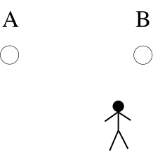
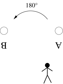
Figure 4: The presence/existence of the observer breaks the symmetry of the physical configuration under 180⁰ rotation.

Figure 5: The observer does not rotate. Now the rotated situation is not equivalent to the previous one.

There is therefore a choice which corresponds to the maximum of entropy. The real situation can be schematically depicted as follows. The “empty space” is something like in figure 6, in which the two dots, distinguished by the shadowing, represent the observer, i.e. not only “the person who observes”, but more crucially “the object (person or device) which can distinguish between configurations”.

Figure 6: The presence of an observer able to detect a motion according to a group action is something that breaks the symmetry of the universe under this group, otherwise the action would not be detectable. Here we represent the observer as something that distinguishes A from B.

Now we add the experiment, figure 7. In this case, the previous figures 3 and 3 correspond to figures 9 and 9.

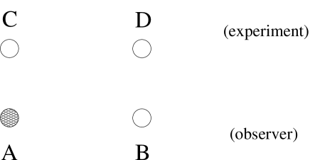
Figure 7: In the presence of an observer, here represented by the points A and B, even with a “symmetric” system, the points C, D, the universe is no more symmetric. Points C and D can be identified, by saying that C is the one closer to A, D the one closer to B.

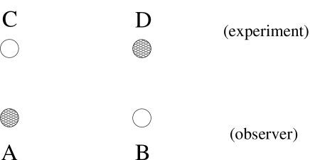
Figure 8: The analogous of figure 3 in the presence of an observer.

Figure 9: The analogous of figure 3 in the presence of an observer.

It should be clear that entropy in the configuration of figure 9 is not the same as in the configuration of figure 9. This means that the observer “breaks the symmetries” in the universe, it decides that this one, namely figure 6, is the actual configuration of the universe, i.e. the one contributing with the highest weight to the appearance of the universe, while the one obtained by exchanging A and B is not.

The observer is itself part of the universe, and the symmetric situation of the ideal problem of the double slit is only an abstraction. In our approach, it is the very presence of an observer, i.e. of an asymmetrical configuration of space geometry, what removes the degeneracy of the physical configurations, thereby solving the paradox of equivalent probabilities of ordinary quantum mechanics. In this perspective there are indeed no “probabilities” at all: the universe is the superposition of configurations in the same sense as wave packets are superpositions of elementary (e.g. plane) waves; real waves, not “probability wave functions”. This means also that mean values, given by 2.36, are sufficiently “picked”, so that the universe doesn’t look so “fuzzy”, as it would if rather different configurations contributed with a similar weight. Indeed, the fuzziness due to a small change in the configuration, leading to a smearing out of the energy/curvature distribution around a space region, corresponds to the Heisenberg’s uncertainty, section 3. The two points on the target plate correspond to a deeply distinguished asset of the energy distribution, the curvature of space, whose distinction is well above the Heisenberg’s uncertainty.

When objects, i.e. special configurations of space and curvature, are disentangled beyond the “Heisenberg’s scale”, “randomness” and “unpredictability” are rather a matter of the infinite number of variables/degrees of freedom which concur to determine a configuration, i.e., seen from a dynamical point of view, “the path of mean configurations”, their time evolution. In itself, this universe is though deterministic. Or, to better say, “determined”. “Determined” is a better expression, because the universe at time $N^{\prime}\sim{\cal T}^{\prime}={\cal T}+\delta{\cal T}\sim N+1$ cannot be obtained by running forward the configurations at time $N\sim{\cal T}$. The universe at time ${\cal T}+\delta{\cal T}$ is not the “continuation”, obtained through equations of motion, of the configuration at time ${\cal T}$; it is given by the weighted sum of all the configurations at time ${\cal T}+\delta{\cal T}$, as the universe at time ${\cal T}$ was given by the weighted sum of all the configurations at time ${\cal T}$. In the large $N$ limit, we can speak of “continuous time evolution” only in the sense that for a small change of time, the dominant configurations correspond to distributions of geometries that don’t differ that much from those at previous time. With a certain approximation we can therefore speak of evolution in the ordinary sense of (differential, or difference) time equations. Strictly speaking, however, initial conditions don’t determine the future.

Being able to predict the details of an event, such as for instance the precise position each electron will hit on the plate, and in which sequence, requires to know the function “entropy” for an infinite number of configurations, corresponding to any space dimensionality at fixed ${\cal T}\approx N$, for any time ${\cal T}$ the experiment runs on. Clearly, no computer or human being can do that. If on the other hand we content ourselves with an approximate predictive power, we can roughly reduce physical situations to certain ideal schemes, such as for instance “the symmetric double slit” problem. Of course, from a theoretical point of view we lose the possibility of predicting the position the first electron will hit the target (something anyway practically impossible to do), but we gain, at the price of introducing symmetries and therefore also concepts like “probability amplitudes”, the capability of predicting with a good degree of precision the shape an entire beam of electrons will draw on the plate. We give up with the “shortest scale”, and we concern ourselves only with an “intermediate scale”, larger than the point-like one, shorter than the full history of the universe itself. The interference pattern arises as the dominant mean configuration, as seen through the rough lens of this “intermediate” scale.

4.2 Going to the continuum

For $N$ sufficiently large, it is not only possible but convenient to map to a description on the continuum, because this not only makes things easier from a computational point of view, but also better corresponds to the way the physical world shows up to us, or, more precisely, to the interpretation we are used to give of it. This however does not mean that the description on the continuum is the most fundamental one of the physical world (see discussion of section 7.9).

If we want to pass to a description in terms of continuous variables, we must introduce a “length” to be used as a measure: in the continuum, lengths must be measured in terms of a given unit. Differently from the discrete formulation, in which all quantities: the extension of space, the amount of “energy”, the “time”, could be measured in terms of “number of cells”, in the continuum we must a priori introduce a distinguished unit of measure for any type of measurable quantity. To start with, we must introduce a unit of length, that we call $\ell$. This not only serves as a measure, but it can be chosen to coincide with the elementary size, the radius of the unit cell. In this way, we introduce what we call the “Planck length”, $\ell_{\rm Pl}$.

Energies and momenta are conjugate to space lengths, relation 2.47, and the natural unit in which they are measured is the inverse of the Planck length. This leads to the introduction of the Planck Mass $m_{\rm Pl}$ and the unit of conversion between the energy/momentum and space/time scale, the Planck constant $\hbar$ according to the relation:

$$\left[E,P\right]\,\sim\,{1\over\left[R,t\right]}~{}\leadsto~{}m_{\rm Pl}\,\stackrel{{\scriptstyle\rm def}}{{\equiv}}\,{\hbar\over\ell_{\rm Pl}}\,.$$ (4.54)

This corresponds to the usual relation between these quantities, apart from the fact that here doesn’t appear any power of the “speed of light”. In fact, till now we have paired the concepts of energy/momentum/mass because we have not yet distinguished the unit of measure of time from the one of space. Indeed, were all the objects either massless, or permanently at rest, this distinction would be unnecessary. We need to disentangle time from space in order to measure the rate of expansion of objects, “inhomogeneities” in the average geometry of space, as compared to the rate of the expansion of the space itself. As discussed, non-trivial massive objects correspond to subregions that spread out at particular rates, giving therefore rise to a full spectrum of non-trivial “speeds”. We measure these speeds in terms of $c$, the rate of expansion of the radius of the three-sphere with respect to $N$, intended as the time. In section 5.1 we will discuss how this can be identified with the “speed of light in the vacuum”. Obviously, the formulation in terms of discrete numbers and combinatorics corresponds to a choice of units for which all these “fundamental constants” are 1.

From the perspective of a theory on the continuum, in themselves these scales could be considered as free parameters. One could think to be forced to introduce them as regulators, but that in principle they are free to take any possible value. However, being $\ell$ the unit in which the length of space is measured, by varying it one varies the “unit of volume”, or equivalently “the size of the point”, $v$. When considering the full span of volumes $V$ we obtain a series of equivalent sets describing the same system, equivalent histories of the universe. Running in the set $\{V/v\}$ by letting both $V$ and $v$ take any possible value results in a redundancy reproducing an infinite number of times the same situation. Similar arguments hold for the Planck constant $\hbar$ and the speed of expansion $c$. In particular, fixing the speed of expansion to a constant $c$ allows to establish a bijective map between the time $t$ and the volume $V$ of the three-spheres. Varying the map $t\to V$ through a change of $c$ would lead to an over-counting in the “history of the universe” . In summary, we would have classes of universes, parametrized by the values of $c$ and $\ell_{\rm Pl}$. The real, effective phase space is therefore the coset:

$$[{\rm eff.~{}phase~{}space}]\,=\,[{\rm phase~{}space}]\Big{/}\{c\},\{\ell_{\rm Pl}\}\,.$$ (4.55)

When passing to the continuum, at large $N$, we must therefore look for a mapping of the combinatoric problem to a description in terms of continuous geometry, which i) contains as built-in the notion of minimal length, finite speed of propagation of information, i.e. locality of physics, in which ii) energies are related to space extensions through relations such as 2.47, and in which iii) the “evolution” is labeled through a correspondence between configurations and a parameter that we call “time”. Through the relation between this parameter and the curvature, or the “radius” of the maximally entropic configurations, this parameter too can be viewed as a coordinate. Measuring also time in terms of unit cells, the same units we use to measure the space, corresponds to fixing the “speed of expansion” to 1 (later on we will see how this can be seen as the “speed of light”).

5 Relativity

As we discussed in sections 2.1 and 2.6, although the volume of the target spaces of the “unit of energy cells” is eventually considered infinite, $V\to\infty$, at any finite time the dominant configuration of the universe corresponds to a three-sphere of radius $N\sim{\cal T}$. The configurations which correspond to a geometry not bounded within a region of radius $N\sim{\cal T}$, nor three-dimensional, contribute in the form of quantum perturbations: they all fall under the “cover” of the Uncertainty Principle, and are related to what we interpret as the quantum nature of physical phenomena. In other words, this means that at any time ${\cal T}$ we indeed do see an infinitely-extended universe, but this can be reduced to the ordinary geometric interpretation of space only up to a distance ${\cal T}$.

• The space “outside” the horizon is certainly infinitely extended, and somehow we see it, but it contributes to our perception and measurements only for an “uncertainty” of mean values, accounted for by the Heisenberg’s uncertainties.

From a classical point of view, at any finite time ${\cal T}$ what we call “space” in the ordinary sense is of finite extension: it exists only up to a radius $R\sim{\cal T}\sim N$. This is for us the extension of the ”classical” space. In the following we want to see how in this space Einstein’s special (and general) relativity are implied as a particular limit.

5.1 From the speed of expansion of the universe to a maximal speed for the propagation of information

The classical space corresponds to a universe of radius $\sim N$ at time $N$, with total energy also $N$. It expands at speed $1$. Indeed, we can introduce a factor of conversion from time to space, $c$, and say that, by choice of units, we set the speed of expansion to be $c=1$. We want to see how this is also the maximal speed for the propagation of information within the classical space. It is important to stress that all this refers only to the classical space as we have defined it, because only in this sense we can say that the universe is three dimensional: the sum 2.35 contains in fact also configurations in which higher speeds are allowed (we may call them “tachyonic” configurations), along with configurations in which it is not even clear what is the meaning of speed of propagating information in itself, as there is no recognizable information at all, at least in the sense we usually intend it.

Indeed, when we say we get information about, say, the motion of a particle, or a photon, we intend to speak of a non-dispersive wave packet, so that we can say we observe a particle, or photon, that remains particle, or photon, along its motion . Let’s consider the simplified case of a universe at time $N$ containing only one such a wave packet , as illustrated in figure 5.56, where it is represented by the shadowed cells, and the space is reduced to two dimensions.

(5.56)

Consider now the evolution at the subsequent instant of time, namely after having progressed by a unit of time. Adding one point, $N\to N+1$, does produce an average geometry of a three sphere of radius $N+1$ instead of $N$. In the average, it is therefore like having added $4\pi N^{2}$ “points”, or unit cells. Remember that we work always with an infinite number of cells in an unspecified number of dimensions; when we talk of universe in three dimensions within a region of a certain radius, we just talk of the dominant geometry. Let’s suppose the position of the wave packet jumps by steps (two cells) back, as illustrated in figure 5.57. Namely, as time, and consequently also the radius of the universe, progresses by one unit, the packet moves at higher speed, jumping by two units:

(5.57)

Consider now the case in which the packet jumps by just one unit, as in figure 5.58 here below:

(5.58)

The entropy of this latter configuration, intermediate between the first and second one, cannot be very different from the one of the second configuration, figure 5.57, in which the packet jumps by two steps, because that was supposed to be the dominant configuration at time $N+1$, and therefore the one of maximal entropy. Indeed, by “continuity” it must interpolate between step 2 and the configuration at time $N$, that was also supposed to be a configuration of maximal entropy. Therefore, the actual appearance of the universe at time $N+1$ must be somehow a superposition of the configurations 2 and 3, thereby contradicting our hypothesis that the wave packet is non-dispersive . Therefore, the wave packet cannot jump by two steps, and we conclude that the maximal speed allowed is that of expansion of the radius of the universe itself, namely, $c$.

According to this theoretical framework, the reason why we have a universal bound on the speed of light is therefore that light carries what we call classical information. Information about whatever kind of event tells about a change of average entropy of the observed system, of the observer, and what surrounds and connects them too. The rate of transfer/propagation of information is therefore strictly related to the rate of variation of entropy. Variation of entropy is what gives the measure of time progress in the universe. Any vector of information that “jumps” steps of the evolution of the universe, going faster than its rate of entropy variation, becomes therefore dispersive, looses information during its propagation. Light must therefore propagate at most at the rate of expansion of space-time (i.e. of the universe itself). Namely, at the rate of the space/time conversion, $c$.

5.2 The Lorentz boost

Let’s now consider physical systems that can be identified as “massive particles”, i.e. localizable and which exist also “at rest”, therefore travelling at speeds always lower than $c$. Since the phase space has a multiplicative structure, and entropy is the logarithm of the volume of occupation in this space, it is possible to separate for each such a system the entropy into the sum of an internal, “rest” entropy, and an external, “kinetic” entropy. The first one refers to the structure of the system in itself, that can be a point-like particle or an entire laboratory . The second one refers to the relation/interaction of this system with the environment, the external world: its motion, the accelerations and external forces it experiences, etc.

Let us for a moment abstract from the fact that the actual configuration of the universe implied by 2.35 at any time describes a curved space. In other words, let’s neglect the so called “cosmological term”. This approximation can make sense at large $N$, as is the case of the present-day physics, a fact that historically allowed to introduce special relativity and Lorentz boosts before addressing the problem of the cosmological constant. Let us also assume we can just focus our attention on two observers sitting on two inertial frames, $A$ and $A^{\prime}$, moving at relative speed $v$, neglecting everything else . For what above said, $v<1$. An experiment is the measurement of some event that, owing to the fact that happening of something means changing of entropy and therefore is equivalent to a time progress, gives us the perception of having taken place during a certain interval of time. Let us consider an experiment, i.e. the detection of some event, taking place in the co-moving frame of $A^{\prime}$, as reported by both the observer at rest in $A$, and the one at rest in $A^{\prime}$ (from now on we will indicate with $A$, and $A^{\prime}$, indifferently the frame as well as the respective observer). Let’s assume we can neglect the space distance separating the two observers, or suppose there is no distance between them . For what above said, such a detection amounts in observing the increase of entropy corresponding to the occurring of the event, as seen from $A$, and from $A^{\prime}$ itself. Since we are talking of the same event, the overall change of entropy will be the same for both $A$ and $A^{\prime}$. One would think there is an “absolute” time interval, related to the evolution of the universe corresponding to the change of entropy due to the event under consideration. However, the story is rather different as soon as we consider time measurements of this event, as reported by the two observers, $A$ and $A^{\prime}$. The reason is that the two observers will in general attribute in a different way what amount of entropy change has to be considered a change of entropy of the “internal” system, and which amount refers to an “external” change. Proper time measurements have to do with the internal change of entropy. For instance, consider the entropy of all the configurations contributing to form, say, a clock. The part of phase space describing the uniform motion of this clock will not be taken into account by an observer moving together with the clock, as it will not even be measurable. This part will however be considered by the other observer. Therefore, when reporting measurements of time intervals made by two clocks, one co-moving with $A$, and one seen by $A$ to be at rest in $A^{\prime}$, owing to a different way of attributing elements within the configurations building up the system, between “internal” and “external”, we will have in general two different time measurements. Let us indicate with $\Delta S$ the change of entropy as it is observed by $A$. We can write:

$$\Delta S\,(\equiv\Delta S(A)) = \Delta S({\rm internal}\,=\,{\rm at\,rest})\,+\,\Delta S({\rm external})$$ (5.59)

$$= \Delta S(A^{\prime})\,+\,\Delta S_{\rm Kinetic}(A)\,,$$ (5.60)

with the identifications $\Delta S({\rm internal}\,=\,{\rm at\,rest})\equiv\Delta S(A^{\prime})$ and $\Delta S({\rm external})\equiv\Delta S_{\rm Kinetic}(A)$. In section 2.2 we discussed how the entropy of a three sphere is proportional to $N^{2}=E^{2}$. This is therefore also the entropy of the average, classical universe, that in the continuum limit, via the identification of total energy with time, can be written as:

$$S\;\propto\;\left(c{\cal T}\right)^{2}\,,$$ (5.61)

where ${\cal T}$ is the age of the universe. This relation matches with the Hawking’s expression of the entropy of a black hole of radius $r=c{\cal T}$ [11, 12]. It is not necessary to write explicitly the proportionality constant in (5.61), because we are eventually interested only in ratios of entropies. During the time of an event, $\Delta t$, the age of the universe passes from ${\cal T}$ to ${\cal T}+\Delta t$, and the variation of entropy, $\Delta S=S({\cal T}+\Delta t)-S({\cal T})$, is:

$$\Delta S\;\propto\;\left(c\Delta t\right)^{2}\,+\,c^{2}{\cal T}^{2}\left({2\Delta t\over{\cal T}}\right)\,.$$ (5.62)

The first term corresponds to the entropy of a “small universe”, the universe which is “created”, or “opens up” around an observer during the time of the experiment, and embraces within its horizon the entire causal region about the event. The second term is a “cosmological” term, that couples the local physics to the history of the universe. The influence of this part of the universe does not manifest itself through elementary, classical causality relations within the duration of the event, but indirectly, through a (slow) time variation of physical parameters such as masses and couplings, (we refer to [1] for a discussion of the time dependence of masses and couplings. See also [2]). In the approximation of our abstraction to the rather ideal case of two inertial frames, we must neglect this part, concentrating the discussion to the local physics. In this case, each experiment must be considered as a “universe” in itself. Let’s indicate with $\Delta t$ the time interval as reported by $A$, and with $\Delta t^{\prime}$ the time interval reported by $A^{\prime}$. In units for which $c=1$, and omitting the normalization constant common to all the expressions like 5.61 , we can therefore write:

$$\Delta S(A)\rightarrow\langle\Delta S(A)\rangle\approx(\Delta t)^{2}\,,$$ (5.63)

whereas

$$\Delta S(A^{\prime})\rightarrow\langle\Delta S(A^{\prime})\rangle\approx(\Delta t^{\prime})^{2}\,,$$ (5.64)

and

$$\Delta S_{\rm Kinetic}(A)~{}=~{}(v\,\Delta t)^{2}\,.$$ (5.65)

These expressions have the following interpretation. As seen from $A$, the total increase of entropy corresponds to the black hole-like entropy of a sphere of radius equivalent to the time duration of the experiment. Since $v=c=1$ is the maximal “classical” speed of propagation of information, all the classical information about the system is contained within the horizon set by the radius $c\Delta t=\Delta t$. However, when $A$ attempts to refer this time measurement to what $A^{\prime}$ could observe, it knows that $A^{\prime}$ perceives itself at rest, and therefore it cannot include in the computation of entropy also the change in configuration due to its own motion (here it is essential that we consider inertial systems, i.e. constant motions). “$A$” separates therefore its measurement into two parts, the “internal one”, namely the one involving changes that occur in the configuration as seen at rest by $A^{\prime}$ (a typical example is for instance a muon’s decay at rest in $A^{\prime}$), and a part accounting for the changes in the configuration due to the very being $A^{\prime}$ in motion at speed $v$. If we subtract the internal changes, namely we think at the system at rest in $A^{\prime}$ as at a point without meaningful physics apart from its motion in space , the entire information about the change of entropy is contained in the “universe” given by the sphere enclosing the region of its displacement, $v^{2}(\Delta t)^{2}~{}=~{}\Delta S_{\rm Kinetic}(A)$. In other words, once subtracted the internal physics, the system behaves, from the point of view of $A$, as a universe which expands at speed $v$, because the only thing that happens is the displacement itself, of a point otherwise fixed in the local universe (see figure 10).

Figure 10: During a time $\Delta t$, the pure motion “creates” a universe with an horizon at distance $\Delta x=v\Delta t$ from the observer. As seen from the rest frame, this part of the physical system does not exist. The “classical” entropy of this region is given by the one of its dominant configuration, i.e. it corresponds to the entropy of a black hole of radius $\Delta x$.

Inserting expressions 5.63–5.65 in 5.60 we obtain:

$$(\Delta t)^{2}~{}=~{}{(\Delta t^{\prime})^{2}\over 1-v^{2}}\,,$$ (5.66)

that is:

$$\Delta t~{}=~{}{\Delta t^{\prime}\over\sqrt{1-v^{2}}}\,.$$ (5.67)

The time interval as measured by $A$ results to be longer by a factor $(\sqrt{1-v^{2}})^{-1}$ than as measured by $A^{\prime}$. We stress that, when we use expressions like “as seen from”, “it observes” and alike, we intend them in an ideal sense, not in the concrete sense of “detecting a light ray coming from what is observed”. We stress that in this argument the bound on the speed of information, and therefore of light, enters on when we write the variation of entropy of the “local universe” as $\Delta S=(c\Delta t)^{2}$. If $c\to\infty$, namely, if within a finite interval of time an infinitely extended causal region opens up around the experiment, both $A$ and $A^{\prime}$ turn out to have access to the full information, and therefore $\Delta t=\Delta t^{\prime}$. This means that they observe the same overall variation of entropy.

5.2.1 the space boost

In this framework we obtain in quite a natural way the Lorentz time boost. The reason is that, for us, time evolution is directly related to entropy change, and we identify configurations (and geometries) through their entropy. The space length is somehow a derived quantity, and we expect also the space boost to be a secondary relation. Indeed, it can be easily derived from the time boost, once lengths and their measurements are properly defined. However, these quantities are less fundamental, because they are related to the classical concept of geometry. We could produce here an argument leading to the space boost. However, this would basically be a copy of the classical derivation within the framework of special relativity. The derivation of the time boost through entropy-based arguments opens instead new perspectives, allowing to better understand where relativity ends and quantum physics starts. Or, to better say, it provides us with an embedding of this problem into a scenario that contains both these aspects, relativity and quantization, as particular cases, to be dealt with as useful approximations.

5.3 General time coordinate transformation

Lorentz boosts are only a particular case of a more general transformation. They are valid when systems are not accelerated; in particular, when they are not subjected to a gravitational force. Traditionally, we know that the general coordinate transformation has to be found within the context of General Relativity; in that case the measure of time lengths is given by the time-time component of the metric tensor. In the absence of mixing with space boosts, i.e., with a diagonal metric, we have:

$$(ds)^{2}~{}=~{}g_{00}(dt)^{2}\,.$$ (5.68)

As the metric depends on the matter/energy content through the Einstein’s Equations:

$${\cal R}_{\mu\nu}-{1\over 2}g_{\mu\nu}{\cal R}\,=\,8\pi G_{N}T_{\mu\nu}\,,$$ (5.69)

$g_{00}$ can be computed when we know the energy of the system. For instance, in the case of a particle of mass $m$ moving at constant speed $\vec{v}$ (inertial motion), the energy, the “external” energy, is the kinetic energy ${1\over 2}mv^{2}$, and we recover the $v^{2}$-dependence of the Lorentz boost .

In the simple case of the previous section, we have considered the physical system of the wave packet as decomposed into a part experiencing an “internal” physics, and a part which corresponds to the point of view of the center of mass, that is a part in which the complex internal physics is dealt with as a point-like particle. The Lorentz boost has been derived as the consequence of a transformation of entropies. Indeed, our coordinate transformation is based on the same physical grounds as the usual transformation of General Relativity, based on a metric derived from the energy tensor. Let us consider the transformation from this point of view: although imprecise, the approach through the linear approximation helps to understand where things come from. In the linear approximation, where one keeps only the first two terms of the expansion of the square-root $\sqrt{1-v^{2}/c^{2}}$, the Lorentz boost can be obtained from an effective action in which in the Lagrangian appear the rest and the kinetic energy. These terms correspond to the two terms on the r.h.s. of equation 5.60. Entropy has in fact the dimension of an energy multiplied by a time . Approximately, we can write:

$$\Delta S~{}\simeq~{}\Delta E\Delta t\,,$$ (5.70)

where $\Delta E$ is either the kinetic, or the rest energy. The linear version of the Lorentz boost is obtained by inserting in (5.70) the expressions $\Delta E_{rest}=m$ and $\Delta E_{kinetic}={1\over 2}mv^{2}$. In this case, the linearization of entropies lies in the fact that we consider the mass a constant, instead of being the full energy of the “local universe” contained in a sphere of radius $\Delta t$, i.e. the energy (mass) of a black hole of radius $\Delta t$: $m=\Delta E=\Delta t/2$.

In our theoretical framework, the general expression of the time coordinate transformation is:

$$(\Delta t^{\prime})^{2}~{}=~{}\langle\Delta S^{\prime}(t)\rangle\,-\,\langle\Delta S^{\prime}_{external}(t)\rangle\,.$$ (5.71)

Here $\Delta S^{\prime}(t)$ is the total variation of entropy of the “primed” system as measured in the “unprimed” system of coordinates: $\langle\Delta S^{\prime}(t)\rangle\,=\,(\Delta t)^{2}$. We can therefore write expression 5.71 as:

$$(\Delta t^{\prime})^{2}~{}=~{}\left[1-\mathcal{G}(t)\right](\Delta t)^{2}\,,$$ (5.72)

where:

$$\mathcal{G}(t)~{}\stackrel{{\scriptstyle\mathrm{def}}}{{=}}~{}{\Delta S^{\prime}_{external}(t)\over(\Delta t)^{2}}\,.$$ (5.73)

With reference to the ordinary metric tensor $g_{\mu\nu}$, we have:

$$\mathcal{G}(t)~{}=~{}1-g_{00}\,.$$ (5.74)

$\Delta S^{\prime}_{external}(t)$ is the part of change of entropy of $A^{\prime}$ referred to by the observer $A$ as something that does not belong to the rest frame of $A^{\prime}$. It can be the non accelerated motion of $A^{\prime}$, as in the previous example, or more generally the presence of an external force that produces an acceleration. Notice that the coordinate transformation 5.72 starts with a constant term, 1: this corresponds to the rest entropy term expressed in the frame of the observer. For the observer, the new time metric is always expressed in terms of a deviation from the identity.

By construction, 5.73 is the ratio between the metric in the system which is observed and the metric in the system of the observer. From such a coordinate transformation we can pass to the metric of space-time itself, provided we consider the coordinate transformation between the metric $g^{\prime}$ of a point in space-time, and the metric of an observer which lies on a flat reference frame, whose metric is expressed in flat coordinates. We have then:

$$1\,-\,\mathcal{G}(t)~{}=~{}{g_{00}^{(\prime)}\over g^{(0)}_{00}\,=\eta_{00}=1}\,.$$ (5.75)

As soon as this has been clarified, we can drop out the denominator and we rename the primed metric as the metric tout court.

5.4 General Relativity

Once the measurement of lengths is properly introduced, as derived from a measurement of configurations along the history of the system, it is possible to extend the relations also to the transformation of space lengths. This gives in general the components of the metric tensor as functions of entropy and time. In classical terms, whenever this reduction is possible, this can be rephrased into a dependence on energy (energy density) and time. They give therefore a generalized, integrated version of the Einstein’s Equations. Let’s see this for the time component of the metric. We want to show that the metric $g_{00}$ of the effective space-time corresponds to the metric of the distribution of energy in the mean space, i.e., in the classical limit of effective three-dimensional space as it arises from 2.35. This will mean that the geometry of the motion of a particle within this space is the geometry of the energy distribution. In particular, if the energy is distributed according to the geometry of a sphere, so it will be the geometry of space-time in the sense of General Relativity. To this regard, we must remember that:

${\rm i})$ All these arguments make only sense in the “classical limit” of our scenario, namely only in an average sense, where the universe is dominated by a configuration that can be described in classical geometric terms. It is in this limit that the universe appears as three dimensional. Configurations which are in general non three-dimensional, non-geometric, possibly tachyonic, and, in any case, configurations for which General Relativity and Einstein Equations don’t apply, are covered under the “un-sharping” relations of the Uncertainty Principle. All of them are collectively treated as “quantum effects”;

${\rm ii})$ In the classical limit, nothing travels at a speed higher than $c$. As during an experiment no information comes from outside the local horizon set by the duration of the experiment itself, to cause some (classical) effects on it, any consideration about the entropy of the configuration of the object under consideration can be made “local” (tachyonic effects are taken into account by quantization). That means, when we consider the motion of an object along space we can just consider the local entropy, which depends on, and is determined by, the energy distribution around the object.

Having these considerations in mind, let us consider the motion of a particle, or, more precisely, a non-dispersive wave-packet, in the mean, three-dimensional, classical space. Consider to perform a (generally point-wise) coordinate transformation to a frame in which the metric of the energy distribution external to the system intrinsically building the wave packet in itself is flat, or at least remains constant. As seen from this set of frames, along the motion there is no change of the (local) entropy around the particle, and the right hand side of 5.73 vanishes, implying that also the metric of the motion itself remains constant (remember that 5.73 in this case gives the ratio between metrics at different points/times). This means that the metric of the energy distribution and the metric of the motion are the same, and proves the equivalence of 5.71 and 5.73 with the Einstein’s equations 5.69.

If on the other hand we keep the frame of the observer fixed, and we ask ourselves what will be the direction chosen by the particle in order to decide the steps of its motion, the answer will be: the particle “decides” stepwise to go in the direction that maximizes the entropy around itself. Let us consider configurations in which the only property of particles is their mass (no other charges), so that entropy is directly related to the “energy density” of the wave packet. In this case, between the choice of moving toward another particle, or far away, the system will proceed in order to increase the energy density around the particle. Namely, moving the particle toward, rather than away from, the other particle, in order to include in its horizon also the new system. This is how gravitational attraction originates in this theoretical framework.

In order to deal with more complicated cases, such as those in which particles have properties other than just their mass (electro-magnetic/weak/strong charge), we need a more detailed description of the phase space. In principle things are the same, but the appropriate scenario in which all these aspects are taken into account is the one in which these issues are phrased and addressed within a context of (quantum) String Theory. This analysis, first presented in Ref. [2], will be discussed in Ref. [1] in an updated and corrected form.

5.5 The metric around a black hole

Let us consider once more the general expression relating the evolution of a system as is seen by the system itself, indicated with $A^{\prime}$, and by an external observer, $A$, expressions 5.59 and 5.60. In the large-scale, classical limit, the variations of entropy $\Delta S(A)$ and $\Delta S(A^{\prime})$ can be written in terms of time intervals, as in 5.63 and 5.64, in which $t$ and $t^{\prime}$ are respectively the time as measured by the observer, and the proper time of the system $A^{\prime}$. In this case, as we have seen expression 5.60 can be written as $(\Delta t^{\prime})^{2}=(\Delta t)^{2}\,-\,\langle\Delta S^{\prime}_{\rm external}(t)\rangle$ (see expression 5.71), and the temporal part of the metric is given by:

$$g_{00}~{}=~{}{\langle\Delta S^{\prime}_{\rm external}(t)\rangle\over(\Delta t)^{2}}\,-\,1\,.$$ (5.76)

As long as we consider systems for which $g_{00}$ is far from its extremal value, expression 5.76 constitutes a good approximation of the time component of the metric. However, a black hole does not fall within the domain of this approximation. According to its very (classical) definition, the only part we can probe of a black hole is the surface at the horizon. In the classical limit the metric at this surface vanishes: $g_{00}\to 0$ (an object falling from outside toward the black hole appears to take an infinite time in order to reach the surface). This means,

$$\langle\Delta S_{\rm external}\rangle~{}\approx~{}\propto\,\left(\Delta t\right)^{2}\,.$$ (5.77)

However, in our set up time is only an average, “large scale” concept, and only in the large scale, classical limit we can write variations of entropy in terms of progress of a time coordinate as in 5.63 and 5.64. The fundamental transformation is the one given in expressions 5.59, 5.60, and the term $g_{00}$ has only to be understood in the sense of:

$$\Delta S(A^{\prime})\,\longrightarrow\,\langle\Delta S(A^{\prime})\rangle\,\equiv\,\Delta t^{\prime}g_{00}\Delta t^{\prime}\,.$$ (5.78)

The apparent vanishing of the metric 5.76 is due to the fact that we are subtracting contributions from the first term of the r.h.s. of expression 5.60, namely $\Delta S(A^{\prime})$, and attributing them to the contribution of the environment, the world external to the system of which we consider the proper time, the second term in the r.h.s. of 5.60, $\Delta S_{\rm external}(A)$. Any physical system is given by the superposition of an infinite number of configurations, of which only the most entropic ones (those with the highest weight in the phase space) build up the classical physics, while the more remote ones contribute to what we globally call “quantum effects”. Therefore, taking out classical terms from the first term, $\Delta S(A^{\prime})$, the “proper frame” term, means transforming the system the more and more into a “quantum system”. In particular, this means that the mean value of whatever observable of the system will receive the more and more contribution by less localized, more exotic, configurations, thereby showing an increasing quantum uncertainty. In particular, the system moves toward configurations for which $\Delta x\rightarrow\gg 1/\Delta p$. Indeed, one never reaches the condition of vanishing of 5.78, because, well before this limit is attained, also the notion itself of space, and time, and three dimensions, localized object, geometry, etc…, are lost. The most remote configurations in general do not describe a universe in a three-dimensional space, and the “energy” distributions are not even interpretable in terms of ordinary observables. At the limit in which we reach the surface of the horizon, the black hole will therefore look like a completely delocalized object [6].

6 String Theory

In the previous sections we have derived what is in the average the dominant geometry of the universe. To the whole resulting geometry contribute also an infinite bunch of less entropic configurations, responsible for “minor” deviations, “perturbations” of the dominant configuration, what we called “inhomogeneities” of the energy distribution. In order to investigate what kind of perturbations do we have, it is convenient to map the combinatorial problem into a description of the world in terms of propagating fields and particles. This is also a way to make contact with the common approach to physics and observables.

Let us consider the geometry of the universe resulting from 2.35. In its grounds, what we have is a distribution of amounts of energy along space, with the time ordering $E$. The rule of the dynamics is that the universe ”evolves” in such a way that at any time what we have is basically the configuration of maximal entropy, plus “quantum” corrections which modulate the smoothness of the dominant geometry into a bunch of propagating and interacting “wave packets”. For small intervals of ”time” $\delta t$, the evolution can be approximated by a continuous evolution, parametrizable in terms of interactions and propagation of fields and particles. Indeed, a priori it is not at all obvious that such a description is possible or makes sense: if wave packets disperse too rapidly, such an approximation does not work. It makes sense only at a sufficiently large age of the universe (large $N$). It is on the other hand important to notice that it remains just an approximation, and that a description in terms of fields, particles and their interactions, whatever this description may be, is not necessarily the only possible description of the physical reality, in the sense that, a priori, one may think to organize the universe described by of 2.35 also in another conceptual framework. Our mental organization in terms of the degrees of freedom of particles and fields is grounded on historical reasons, and finds here a justification in the separation of the physics arising from 2.35 into a dominant configuration plus corrections falling within the domain of the Heisenberg’s Uncertainty. This means that particles and fields that mediate their interactions will be quantum objects. The Heisenberg Uncertainty allows us to keep under control the approximation implicit in this organization of physical phenomena, and account for its lack of precision.

In the world described by 2.35, a map to a description in terms of quantum fields and particles makes only sense “locally”, where locality must be intended not only in the sense of space but also in the sense of time. Any embedding into a theory of time-dependent propagating fields and particles framed in an infinite space-time is only formal: the map must be “updated” at any time of the evolution of the universe, something which can be kept into account by introducing time-dependent masses and couplings.

We want now to see what are the conditions such a map must satisfy in order to faithfully represent the physics of the combinatorial framework. At the end of our discussion, we will conclude that such a map not only exists, but that it is unique, in the sense that the conditions determine it uniquely.

6.1 Mapping to quantum fields

Let us summarize the key points at the base of the map to quantum fields we are looking for.

$\bullet$ A first thing we want to show is that the “canonical” form of the Uncertainty Principle, namely the inequality 3.52 (i.e. in the appropriate normalization $\Delta E\Delta t\geq 1/2$, which in a relativistic context goes together with $\Delta P\Delta x\geq 1/2$), implies, and is implied by, only one dimensionality of space, with a well defined geometry. In our combinatorial construction, we have seen that we obtain a ”classical” D=3 dimensional space, plus the Heisenberg Uncertainty. The dimensionality of space becomes D=3+1 once we implement the ”time” E in a time coordinate suitable for a field theory description. Taking this into account, what we have seen is that:

$${\rm combinatorial~{}scenario}~{}\Rightarrow~{}\left[D=3+1\right]\,\cup\,\left[\Delta E\Delta t\geq 1/2\right]\,.$$ (6.79)

This means also that:

$$\Delta E\Delta t\geq 1/2~{}\Leftrightarrow~{}D=3+1\,.$$ (6.80)

Let us suppose in fact by absurd that $\Delta E\Delta t\geq 1/2\Leftrightarrow D\neq 3+1$. Then, in the sum of the rests considered to derive the uncertainty (see section 3), the ratio between weight of the classical and weights of quantum configurations is different, something that would lead to a different uncertainty. But there is more: $\Delta E\Delta t\geq 1/2$ not only is uniquely related to the dimensionality, but also to the geometry of space, because geometries different from the sphere have different entropy, and therefore different weight, leading to a different uncertainty. This means that the relation $\Delta E\Delta t\geq 1/2$ not only fixes dimension and main geometry, but also the spectrum of the theory.

$\bullet$ A second point to remark is that, if we look for a description of this world in terms of quantum particles with wave-like behavior, their masses must correspond to momenta of a certain space, i.e. to the inverse of appropriate radii. In order to introduce higher masses than just the ”cosmological mass”, given by the inverse of the radius of the universe, we must introduce an internal space. In this way, instead of $m=1/R$ we can have $m=1/\langle R\rangle$, where $\langle R\rangle=\sqrt[p]{R\times r_{1}\times r_{2}\cdots\times r_{p-1}}$, the $r_{i}$, $1\leq i\leq p-1$ being internal radii. In the particular case in which all these turn out to be of elementary (= minimal) size, $r_{i}=1$ $\forall i$, the mass expression reduces to $m_{(p)}=1/\sqrt[p]{R}$. We need therefore a relativistic quantum field theory with internal dimensions.

6.1.1 How many dimensions do we need?

How many internal dimensions do we need? We want to describe all the possible perturbations of the geometry of a sphere in three dimensions, as due to fields and particles that propagate in it. Notice that it is not a matter of building a set of fields framed in a certain space, i.e. functions of space-time coordinates. It is a matter of promoting the deformations of the geometry themselves to the role of fields. One may think at a description in terms of vector fields. Once provided with a time coordinate, the three-sphere $\times$ the time coordinate, which can be considered the D = 3+1 “background” space, corresponds to vector fields possessing an $SO(3,1)$ symmetry. However, we must have both bosons and fermions. Fermions are needed because we want a quantum relativistic description of fields. It is relativity what leads to the introduction of spinorial representations of space. This does not mean we need bosons and fermions in equal number, nor even that they must have the same mass (implying supersymmetry of the theory): supersymmetry is not a symmetry of the real world (in the sense of an exact symmetry). In terms of spinorial representations, $SO(3,1)$ is locally isomorphic to $SU(2)\times SU(2)$, a group with 3+3 generators, which, once parametrized in terms of bosonic fields, correspond to a space with six bosonic coordinates. One would like to conclude that, in order to have both a vectorial and a spinorial representation of the background space with all its perturbations we need therefore the original 3+1 plus 3+3 internal coordinates. With six internal dimensions it seems we are sure that whatever internal configuration can be mapped to a configuration of space-time, allowing for a non-trivial (and complete) mapping between the ”fiber” and the ”base” space, ensuring to have a non-degenerate and complete description of all the perturbations. There is however a subtlety: our theory has also a minimal length, ”1”. This “cut-off” can be viewed as a specific value $g_{0}$ of a coupling $g$. Indeed, it is by definition the ”gravitational” coupling of the theory (more on this point later). Unfreezing this one results in a new dimension, $g_{0}=1\to g=x$. We need therefore at least 11 dimensions. Since this space is in general curved, there is one more parameter of the theory, the curvature. This discriminates between geometries, and as such is also part of the definition of the coupling of this geometric field theory. It is not an independent parameter, being a function of all the coordinates. However, this coupling too can be viewed as a coordinate, or, to better say, it may turn out convenient to embed it into a flat, independent coordinate: if we want to give a representation of an 11-dimensional curved space in terms of flat coordinates, we need 12 coordinates .

6.1.2 T-duality

$g=g_{0}=1$ is a self-dual point. Any kind of ”unfreezing”, as a matter of fact simply ”projects” onto one of the two possible decompactifications: either $x<1$ or $x>1$. In the perturbative limit, $x\to 0$ or $x\to\infty$ respectively. This is a real projection, in the sense that at the limit part of the physical content is “lost”: it is in fact not possible to simply establish that a certain value of $g$, say $g=g_{0}$, is the cut off of the theory, the “boundary” value, above or below which the coordinate extends. Setting $g$ to a chosen, finite value $g_{0}$, to be the size in comparison to which all other ones are measured, makes only sense if in the theory we have also non-trivial values of couplings above and below $g_{0}$. Otherwise, in practice $g_{0}$ would be a free, running parameter: its actual value would be meaningless, being possible to scale it out by an unphysical overall rescaling. As we will see, this in practice means that the field theory representation will necessarily have strongly and weakly coupled sectors. In principle, the two decompactification limits, $g\to 0$ and $g\to\infty$, are equivalent. This does not mean that the theory is necessarily invariant under T-duality, as is called the symmetry under inversion of the value of the coordinate (in the case of a coupling, one speaks more properly of S-duality), and indeed it must not be: if it was T-duality invariant, then T-duality would be an unphysical transformation, mapping the theory into itself. From the point of view of the phase space (or of the configurations in the combinatorial scenario), this would mean that all the configurations of the phase space possess this symmetry. The latter could then be reabsorbed into a redefinition of the elements of the phase space, not as single configurations but as classes of configurations, given by the orbits of T-duality. Although not an exact symmetry, it is however essential that the complete theory must contain both the “sectors” related by T-duality, which are non-perturbative with respect to each other. Therefore, in general in a perturbative construction not all the states are visible.

To summarize, what we need is a quantum relativistic field theory which is perturbative in ten dimensions, is endowed with some kind of T-duality mechanism, and accounts for a vectorial and spinorial realization of the fields

Any supersymmetric quantum string theory provides such a realization because, in any of its perturbative realizations, it corresponds to all the above mentioned criteria, and introduces spinors starting from the embedding of what, according to a result of Haag, Sohnius and Lopuszanski (see [15]), is the most general graded Lie algebra compatible with a relativistic quantum field theory. Supersymmetry is in general not a symmetry of the theory derived from 2.35, which is always defined on a finite volume, and is not a symmetry of every string vacuum either. However, perturbative field constructions are always realized in a decompactification limit, and every string vacuum can be constructed by starting from a vacuum which in this limit is supersymmetric, by reduction via projection/compactification on more curved/singular spaces. Therefore, the supersymmetric one is the most symmetric string configuration (supersymmetry is the most general extension of the Poincaré algebra). From the discussion we will present in section 6.2, one derives that this is also the less entropic in the string phase space among the whole tower of derived conpactifications that descend from it. Supersymmetric string theory is therefore the ground construction from which one starts to investigate the mapping of the combinatorial formulation in terms of a description based on quantum relativistic fields.

The existence of a minimal length is naturally embedded in closed string theory through its “T-duality” symmetry in any of its coodinates, which shows up upon compactification onto circles . Type I string is obtained as an orientifold of type II string [16], and as such doesn’t possess an explicit T-duality of target space coordinates upon toroidal compactification. Nevertheless, its physical content is equivalent to the one of the string with T-duality, because one ensures to remain within the space of all the other string constructions by enforcing extra sectors required by cancellation of anomalies. These precisely correspond to what in the other constructions are the “T-dual” or “S-dual” sectors. We will discuss later the issue about uniqueness of string theory, namely the question whether all different types of string construction are indeed slices of the same theory.

Perturbative superstring theory is realized precisely in ten dimensions. The reason why this is the critical dimension is apparently unrelated to the way we predicted this number of dimensions in section 6.1.1. However, the fact that 10 dimensions arise in string theory only once fermions are embedded, through the most general extension of the Poincaré algebra, is a hint on the fact that there must be a deep relation between this property, and the fact that quantum superstring theory bears already built-in in its construction the information that it is the theory “thought of” in order to eventually describe the vectorial and spinorial geometries of a four-dimensional quantum world.

Hidden behind the technicalities of the properties of conformal field theory, there is a deeper level of relations between quantization and dimension of the most general vectorial and spinorial realization of geometries, as discussed in section 6.1.1, which ultimately relies on the logical structure we have introduced through our combinatorial approach. String theory is built as a geometric theory endowed with a quantization principle, which implements the Heisenberg’s Uncertainty Relations, under which all “non-dominant” configurations are “covered”. This procedure encodes therefore a choice of “starting point” for the approximation of the configurations, three space dimensions, plus a rule implementing the ignorance due to the fact of neglecting the rest, the Uncertainty Relations. In our set up, the space/momentum (and time/energy) relations appears precisely in the form of the Heisenberg’s inequality. This is related to a specific choice of the scaling of energy $\sim N$ as compared to the scaling of space, which appeared as the natural one. We expect therefore that quantum string theory should be non-anomalous when built out of a number of coordinates which allows a correspondence of these descriptions. Alternatively, one could think to choose a different relation between “energy” $N$ and radius, or time. We would then get a different uncertainty relation, of the type:

$$(\Delta X)^{\alpha}\Delta p\,\geq\,{1\over 2}\hbar\,,$$ (6.81)

where $\alpha$ is an exponent, $\alpha\neq 1$. In this case, quantum string theory would be non-anomalous in a different number of dimensions.

6.2 Entropy in the string phase space

In order to represent a mapping of our combinatorial problem at any finite time, we must consider also string theory as living on a compact space. This implies that it must be considered in a non-perturbative regime, where, in particular, owing to compactness of the space, supersymmetry is broken. Considering string theory as defined on a compact space, and viewing infinitely extended space only as a limiting case of a compact space, entails a deep change of perspective, full of consequencies for the interpretation of things that we compute in string theory. For instance, owing to the always broken supersymmetry, the string partition function does not vanish. Owing to the lack of translational invariance in the very definition of the theory, there is no inverse four-volume factor in the normalization of mode expansions and therefore on string amplitudes. As a consequence, the vacuum energy one calculates on the string vacuum with the usual techniques of taking the vacuum mean value of the partition function does not compute an energy density but a global energy. In order to obtain the vacuum energy density one must divide this quantity by a volume factor corresponding to the actual radius of the horizon of the universe in the dominant configuration. Precisely this volume factor allows to obtain in a natural way and without fine tuning the correct value of the cosmological constant (see [1], cfr. also [2]).

Consider now the collection of non-equivalent string constructions. In its whole, this ”world of string constructions” is the string counterpart of the phase space of the combinatorial configurations of the universe, of which it constitutes a representation. We will call it the string phase space. The physics of this ”universe” will be obtained by the analogous of 2.35 for string constructions. This means that we will have to take the sum over all string vacua, weighted by their volume of occupation in the string phase space. First of all: what is now the counterpart of keeping fixed the total energy $E$? This cannot be easily identified with the time of the string target space, as in this description time is not compact. In principle, it is possible to consider the target space coordinate “$X_{0}$” as being compact, but this does not solve our problem of correctly mapping the combinatorial problem of summing configurations at fixed total $E$. Indeed, on the combinatorial side $E$ is also the radius of the classical space, i.e. the space on top of which we build up the quantum theory. In that case, fixing the radius means also fixing the volume of space, because the geometry is fixed to be predominantly a three sphere. On the string side, the string target space does not distinguish a priory between three selected space coordinates, the representatives of the three-dimensional physical space, and the coordinates of an “internal” space: they start all on the same footing, and a possible selection of just three as the physical space must come by itself, in the string configuration that dominates in the string phase space, not as an external input. This tells us that, when dealing with string vacua, instead of comparing constructions at fixed $E$, we must compare constructions at fixed volume of the target space, no matter how many dimensions this describes (the concept itself of what are to be considered as dimensions of physical space, and what “internal” dimensions, will be clarified in the following). On the string space, 2.35 becomes therefore:

$${\cal Z}_{V}\,=\,\int_{V}{\cal D}\psi\,{\rm e}^{S(\psi)}\,,$$ (6.82)

where $\psi$ indicates now a whole, non-perturbative string configuration, and $V$ is the volume of the target space, intended as “measured” in the duality-invariant Einstein frame. In order to understand what kind of “universe” comes out of all the possible string configurations we must therefore find out those that correspond to the maximal entropy in the phase space, at any fixed volume.

String configurations on a compact space are obtained by compactifying the target space on certain spaces, which may be continuous and differentiable, or even singular. In any case, a compactification leads to a reduction of the symmetry of the initial theory. This is obvious by construction in the case of orbifolds: the more singular is the orbifold on which the string is compactified, the higher is the amount of symmetry reduction. But also the other kinds of compactifications can be viewed as generalized cases of symmetry reduction, from the most symmetric, and therefore the very initial, geometry of the string target space. In principle, this should be a higher-dimensional sphere. However, owing to the decompactification implicit in any perturbative construction, the sphere unfolds to a flat space (one may think that the coupling coordinate is precisely the curvature of the whole space), and flat is how the space appears perturbatively. In this limit, the most symmetric compactifications are not spheres but tori. The symmetries of the target space reflect then on the entire string spectrum, in the sense that, if the initial and the derived target space have symmetry represented by the groups $G$ and $G^{\prime}$ respectively, such that $G^{\prime}=G/H$, and the initial spectrum has a symmetry $\tilde{G}$, the new spectrum will have a symmetry $\tilde{G}^{\prime}$ such that $\tilde{G}^{\prime}=\tilde{G}/\tilde{H}$, where $\tilde{H}\cong H$. We may say that both $H$ and $\tilde{H}$ are representations of the same group, that for simplicity we call $H$ . Let’s consider the action of the group $H$ on the initial string configuration, that we call $\Psi$, i.e. the action on its target space and on the spectrum. Consider then the configuration $\Psi^{\prime}$ obtained by modding by $H$. Elements $h\in H$ map $\Psi^{\prime}$ to $\Psi^{\prime\prime}=h\Psi^{\prime}$, physically equivalent to $\Psi^{\prime}$, in the sense that, by construction, there is a one-to-one map between $\Psi^{\prime}$ and $\Psi^{\prime\prime}$ which simply re-arranges the degrees of freedom. From a physical point of view, there are therefore $||H||$ ways of realizing this configuration. The occupation in the whole phase space is therefore enhanced by a factor $||H||$ as compared to the one of $\Psi$. By reducing the symmetry of the target space, we have enhanced the possibilities of realizing a configuration in equivalent ways in the string phase space, in the same sense as, in the two-cells example of section 2, by assigning different colours, black and white, we have the possibility of realizing the configuration “one-white/one-black” in more ways than “white-white” or “black-black”. The string construction with the highest entropy will therefore be the one obtained through the highest amount of symmetry reduction.

6.3 Uniqueness of String Theory: summary of line of thinking

We have discussed how the combinatorial scenario introduced in section 2 constitutes the most general logical structure one may think about, and, as such, is therefore unique. We have also seen that it implies a three-dimensional “classical” relativistic world plus quantum corrections, and that, if translated into a description in terms of propagating fields (and particles) it implies a description in terms of quantum strings. However, the uniqueness of the combinatorial scenario does not imply a priori uniqueness of the string scenario. That is, a priori the various types of superstring construction (heterotic, type II, type I) could correspond to separate sets of combinatorial configurations. Eleven dimensional supergravity too could be an a priori unrelated theory (indeed, being gravity in itself not a quantum theory, 11-d supergravity would be only a part of such a theory). Each one of the various string types would generate a chain of “descendants” obtained via compactification and projection (orbifoldization or other kinds of compactification), starting from the most symmetric (supersymmetric) one and going toward the one compactified on the most singular (= less symmetric) space, something that would produce a configuration which would be the one of highest entropy in the string phase space among the configurations of the particular subset corresponding the specific chain of derived string vacua. A priori there could therefore be several “highest entropy” configurations, one for each type of string. Indeed, the evaluation in itself of the weight of a certain configuration in the string phase space, obtained as discussed in section 6.2 via comparison of the volumes of the symmetry groups, is something clearly defined within each family chain. Comparing configurations belonging to different chains of “descendants” is not obviously unambiguous in itself: a priori there could be string vacua of different types possessing the same degree of symmetry reduction. On the other hand, the definition of weight, and entropy of a configuration, becomes unambiguous also in the string phase space once this is put in relation with the phase space of combinatorial configurations, namely once by symmetry of a configuration one intends the symmetry of the full spectrum, i.e. the whole physical content . In this case, it appears clear that equal symmetry means also equal physical content, i.e. complete equivalence of configurations. It appears also clear that, working in a compact target space, for each type of string construction one can reduce the symmetry only until one reaches a minimum of symmetry/maximum of entropy, because the combinatorial is finite, the volume of the maximal symmetry is finite, and cannot be reduced “ad libitum”.

Let us consider the “highest entropy” configurations belonging to two different chains of descendants, $X^{\rm i}_{\rm max}$ and $X^{\rm j}_{\rm max}$, obtained by a reduction from the most symmetric “parent” vacuum, $X^{\rm i}_{0}$ and $X^{\rm J}_{0}$ respectively, through a chain of projections /singularizations of the target space:

$${\rm type\,(i)}:\,X^{\rm i}_{0} \to X^{\rm i}_{\rm max}$$

$${\rm type\,(j)}:\,X^{\rm j}_{0} \to X^{\rm j}_{\rm max}\,.$$

A priori, $X^{\rm i}_{\rm max}\neq X^{\rm j}_{\rm max}$. The question is to see whether $X^{\rm i}_{\rm max}=X^{\rm j}_{\rm max}$, and moreover whether $X^{\rm i}_{\rm max}=X^{\rm j}_{\rm max}=X_{\rm max}$, where $X_{\rm max}$ is the representation in terms of fields of the universe that 2.35 pops out. If $X^{\rm i}_{\rm max}\neq X_{\rm max}$, it means that $X^{\rm i}_{\rm max}$ corresponds to a superposition of combinatorial configurations whose entropy is such that, once summed up as in 2.42–2.45 in order to give the size of the correction to the configuration of maximal entropy among the set $(i)$, they do not reproduce the Heisenberg inequality. They correspond therefore to a different uncertainty relation, giving rise to different quantization rules. That means: starting with a string configuration assumed to be a quantum representation of the combinatorial problem, as implied by the properties of the universe of combinatorial configurations discussed in section 6.1, quantized according to the canonical quantization rules in order to realize an implementation of the Heisenberg inequality, we end up with a vacuum that does not correspond to the rules we imposed on it. This is a contradiction. Therefore, $X^{\rm i}_{\rm max}=X^{\rm j}_{\rm max}=X_{\rm max}$, and the most entropic string vacuum is unique. Going backwards, through the chain of projections/compactifications, to lower entropy configurations of each family, we infer the equivalence of the various string types. It is precisely by enforcing canonical quantization that we produce a string theory possessing uniqueness properties, and make all the a priori different string types equivalent. The same quantization imposes also a well defined number of dimensions for the (perturbative) string construction, precisely the number of dimensions that leads to a 3+1 dimensional universe as the most entropic configuration.

The fact that the most entropic configuration in 2.35 is a classical three-sphere, namely a $SO(4)/SO(3)$ space, characterized by a symmetry which corresponds to a vectorial, not a spinorial, representation of the group of rotations, tells us that spinors, required by relativity in the basic definition of the quantum theory, in the most entropic configuration will eventually be all paired. Indeed, interactions are only mediated by vectorial fields (photon, graviton), which couple with pairs of fermions (think at the interaction with light, $\bar{\psi}/{\!\!\!\gamma}/{\!\!\!\!A}\psi$, and gravity, through the metric which multiplies the entire effective action). In particular, this means that all fermions are massive (the mass term is of the type $m\bar{\psi}\psi$). This prediction is confirmed by a detailed analysis of the physics coming out from 6.82 (for details, see [1]).

6.4 A string path integral

Proceeding as in section 3 it is possible to show that the contribution to 6.82 given by the configurations of non-maximal entropy amounts to a quantity covered by the Heisenberg Uncertainty. Although expressed in a different way, this somehow matches with the fact that, in the Feynman path integral, the contribution of paths which do not extremize the classical action corresponds to the quantum deviation from the classical physics. Indeed, any configuration $\psi_{V}$ contributing to 6.82 describes a “universe” which, along the set of values of $V$, undergoes a pressureless expansion. In this case, the first law of thermodynamics:

$$dQ\,=\,dU\,+\,PdV\,,$$ (6.83)

specializes to:

$$dQ\,=\,dU\,.$$ (6.84)

Plugged in the second law:

$$dS\,=\,{dQ\over T}\,,$$ (6.85)

it gives:

$$dS\,=\,{dU\over T}\,.$$ (6.86)

Here $T$ is the temperature of the universe, defined as the ratio of its entropy to its energy. In the case of the configuration of maximal entropy, the universe behaves, from a classical point of view, as a an expanding, three-dimensional Schwarzschild black hole, and the temperature is proportional to the inverse of its total energy, or equivalently, its radius: $T\,=\,\hbar c^{3}/8\pi GMk$, where $k$ is the Boltzmann constant and $M$ the mass of the universe, proportional to its age according to $2GM\,=\,{\cal T}$. By substituting entropy by energy and temperature in 6.82 according to 6.86, we get:

$${\cal Z}\,\equiv\,\int{\cal D}\psi\;{\rm e}^{\int{dU\over T}}\,,$$ (6.87)

where $U\,\equiv\,U(\psi(T))$. If we write the energy in terms of the integral of a space density, and perform a Wick rotation from the real temperature axis to the imaginary one, in order to properly embed the time coordinate in the space-time metric, we obtain:

$${\cal Z}\,\equiv\,\int{\cal D}\psi\;{\rm e}^{{\rm i}\int d^{4}x\,E(x)}\,.$$ (6.88)

Let’s now define:

$${\cal S}\,\equiv\,\int d^{4}x\,E(x)\,.$$ (6.89)

Although it doesn’t exactly look like, ${\cal S}$ is indeed the Lagrangian Action in the usual sense. The point is that the density $E(x)$ here is a pure kinetic energy term: $E(x)\,\equiv\,E_{k}$. In the definition of the action, we would like to see subtracted a potential term: $E(x)\,=\,E_{k}\,-\,{\cal V}$. However, the ${\cal V}$ term that normally appears in the usual definition of the action, is in this framework a purely effective term, that accounts for the boundary contribution. Let’s better explain this point. What one usually has in a quantum action in the Lagrangian formulation, is an integrand:

$$L\,=\,E_{k}\,-\,{\cal V}\,,$$ (6.90)

where $E_{k}$, the kinetic term, accounts for the propagation of the (massless) fields, and for their interactions. Were the fields to remain massless, this would be all the story. The reason why we usually need to introduce a potential, the ${\cal V}$ term, is that we want to account for masses and the vacuum energy (in other words, the Higgs potential, and the (super)gravity potential). In our scenario, non-vanishing vacuum energy and non-vanishing masses are not produced, as in quantum field theory, through a Higgs mechanism, but arise as momenta of a space of finite extension, acted on by a shift that lifts the zero mode (see Ref. [1]). When we minimize 6.89 through a variation of fields in a finite space-time volume, we get a non-vanishing boundary term due to the non-vanishing of the fields at the horizon of space-time (moreover, we obtain also that energy is not conserved). In a framework in which space-time is considered of infinite extension, as in the traditional field theory, one mimics this term by introducing a potential term ${\cal V}$, which has to be introduced and adjusted “ad hoc”, with parameters whose origin remains obscure .

The passage from the entropy sum over configurations to the path integral is not just a matter of mathematical trickery. It involves first of all the reinterpretation of amplitudes as probability amplitudes. This is on the other hand implemented in the string construction. But besides this, there is something that may look odd at first sight. In the usual quantum (field) theoretical approach, mean values as computed from the Feynman path integral are in general complex numbers, as implied by the rotation on the complex plane leading to a Minkowskian time, $1/T\to it$. Real (probability) amplitudes are obtained by taking the modulus square of them. This means that what we obtain from 6.82, 6.88 is somehow the square of the traditional path integral. This is related to the fact that, in order to build up the fine inhomogeneities of a vectorial representation of space, as implied by the combinatorials of energy distributions, we resort to a spinorial representation of space-time. Roughly speaking, spinors are “square roots” of vectors. Indeed, as discussed in [1] and [2], masses are here originated by a $Z_{2}$ orbifold shift on the string space. This shift gives rise to massive particles by pairing left and right moving spinor modes (spinor mass terms in four dimensions are of the type $m\psi\bar{\psi}$). The $Z_{2}$ orbifold projection halves the phase space by coupling two parts. In terms of the weight in the entropy sum, we have at the exponent a pairing/projection $(S+S)/Z_{2}$, what makes clear that the amplitudes of 6.82 are squares of those of the elementary fields (with “weight” $\exp S$). Had we just a vectorial (bosonic) representation of space, this would not occur, because vectorial (spin 1, or scalar, spin 0) mass terms are of the type $mA^{2}$, $m\varphi^{2}$. That is, a mass pairs with one boson (usually one sees this in terms of dimension of the field).

7 The space-time, and what propagates in it

7.1 Mean values and observables in the string picture

Mean values of observables are computed through the analog of 2.36 for the string representation of the combinatorial problem,  6.82. The quantity 2.36 receives contributions mostly from the configurations with the highest entropy. One may ask what happens if ${\cal O}$ diverges on some non-extremal entropy configuration. In this case, the main contribution to the mean value of the observed quantity could come from seemingly negligible vacua. However, in this theoretical framework physical quantities such as masses, energies, couplings have a value, a “weight” depending on their occupation in the phase space. Therefore, observables cannot “blow up” on rare configurations on the ground of their very basic definition: they acquire a non-negligible contribution from their being in correspondence with (relatively) often realized processes (see discussion in Ref. [1]).

7.2 The scaling of energy and entropy

We want now to compute the scaling of the total energy of the universe (for a detailed computation of the various contributions to this quantity we refer the reader to [1]). In a generic thermodynamical system, once the partition function is known, energy is computed in a simple way by taking its logarithmic derivative with respect to the temperature. The point is however that, for a generic string configuration, it is not obvious how a temperature should be defined, nor clear whether it can be defined at all. In (perturbative) string theory one can consider the so-called ”one-loop partition function”, which is given as the sum at genus one (one loop in string perturbation) over all the states of the theory, weighted with a sign distinguishing their supersymmetry charge . In the case of unbroken supersymmetry (and also in some special cases of formally broken, but in which states with opposite charge exist at any energy level in equal number), the string partition function vanishes. Basically the reason is that the condition for having preserved supersymmetry is the existence of a limit of decompactification of the theory (i.e. the possibility of taking the limit in which the parameter that tunes the breaking of supersymmetry vanishes). This is always a limit of infinite volume, and therefore of vanishing energy density and temperature. In this situation also any thermodynamical partition function vanishes. In a situation in which instead all the coordinates, including the one serving as coupling of the theory, are compact, as is our case, supersymmetry is broken, and the string partition function does not vanish. Its value gives the energy of the string vacuum, i.e. of the string configuration . In our language, this is the energy of the universe. Indeed, as we discuss in appendix E of [1], the string partition function turns out to precisely correspond to the thermodynamical partition function. What in the string approach serves as temperature, namely, a component of the world-sheet parameter , can be identified with a string coordinate. The identification between world-sheet and target space coordinates involves always two string coordinates, namely a space and a time coordinate. The freedom in the choice of the reparametrization of the map between world-sheet and target space reflects a gauge invariance of the theory, which is usually fixed for instance by choosing a light-cone gauge, in which only the space transverse coordinates explicitly appear in the construction. A condition for this identification is that the target space coordinate is not twisted, otherwise we don’t have a string, but the mapping of a segment to a point. Owing to this identification, the integration over the ”temperature” in the string partition function is always an integration over a parameter of order one in string units. Indeed, for the cases of relevance for us, it results to be of order one also in Planck units (string coupling of order one). As a consequence, the logarithmic derivative of the partition function results to be of the same order as the partition function itself. As long as one is just interested in the simple order of magnitude and scaling law of the vacuum energy, one can deal with the string partition function as with the function which computes the vacuum energy, i.e. like the derivative of the thermodynamical partition function. Through the approximation:

$${\partial{\cal Z}/\partial\beta\over{\cal Z}}~{}\approx~{}{{\cal Z}/\beta~{}(\sim 1)\over{\cal Z}}~{}\approx~{}1\,,$$ (7.92)

we obtain therefore that the vacuum energy is of order one. This is however not automatically the energy of the universe at time ${\cal T}>1$: indeed, owing to the identification of the time coordinate of the string target space with the world-sheet time coordinate, 7.92 is only the energy of the universe at time ${\cal T}=1$. In order to obtain the energy at a generic time ${\cal T}>1$, let us first compute the energy density. This is obtained by dividing the total energy by the volume of the target space. In doing this, one must bear in mind that one coordinate of the space has been set to unit size by the reparametrization which allows to trade it for the coordinate of the string world-sheet. For simplicity, if we suppose that the space is $D$-dimensional, and that all coordinates of the physical space are of length $R$, the energy density is:

$$\rho(E)~{}\approx~{}{1\over R^{D-1}}\,,$$ (7.93)

and not $1/R^{D}$. In this computation, $D$ is the number of all the non-twisted space coordinates, including the coupling. In three dimensions (i.e. in four space-time dimensions) this gives $\rho(E)_{D=3}=1/R^{2}$. However, this is not all the story: as long as T-duality along these coordinates is not broken, also energy densities are invariant under this symmetry. Indeed, as long as T-duality is a symmetry, it is not even possible to distinguish the universe at large volume from the one at small volume. Expression 7.93 is in general just the large volume limit of a more complicate expression invariant under inversion of each radius. In any case, since we are interested in the universe at large volume, well beyond the Planck scale, this approximation is justified. In this limit, for any $D$ the total energy is therefore:

$$\langle E\rangle~{}=~{}\int_{V}\rho(E)~{}\approx~{}R\,.$$ (7.94)

If we start with a universe of Planck size (${\cal T}=R_{1}=\ldots=R_{D}=1$) and let the space to be stirred by propagating massless modes (there exists always at least one such, the graviton) we have at any time $R\sim{\cal T}$, and the total energy can be identified with the age of the universe, as in section 2.

The relation 7.94 matches with those of section 2.2. This means that the string compactifications correspond to a black hole-like universe only in three dimensions (higher dimensional black holes have energy and entropy scaling as higher powers of the radius, see for instance [8]). But, more importantly, it means that the analysis of entropies carried out in section 2.2, and the conclusions we derived about the dimension of the space of the configuration of highest entropy, carries over to the string representation. The configuration of highest entropy corresponds therefore to three space dimensions. This comes not unexpected, because, as we pointed out in section 6, quantum string theory is built precisely with ingredients which make of it a representation of the combinatorial problem, and the canonical quantization precisely imposes the number of degrees of freedom leading to a consistent description of the geometries of a three-dimensional space. In [1] we will see that three is precisely the number of space coordinates which are left untwisted in the case of maximal reduction of symmetry, which, as discussed in section 6.2, corresponds to the maximal entropy in the phase space. We will therefore recover in another way the fact that this scenario leads to automatically to a four-dimensional space, without postulating this condition a priori.

As we will discuss in [1], in the string vacuum of highest entropy T-duality is broken. This makes legal talking of energy density of a large volume universe, as distinguished from small volume, and allows to make contact with the geometric description of the universe as implied by 1.1, 2.35.

7.3 “vectorial” and “spinorial” metric

Till now, we have spoken of space-time as the space spanned by the extended, expanding coordinates, whereas the internal coordinates are those which are frozen at a fixed value. This point deserves to be considered more in detail. The question is about what is the meaning of “dimension” of space-time. It can not be just the number of coordinates we label as “$X_{\mu}$”. Indeed, string theory implements coordinates and degrees of freedom in a framework of space-time-dependent fields. However, in the interpretation of our theoretical framework, the dimension of space is given by the number of independent massless fields. In the dynamical representation of the combinatoric problem on the continuum, the expansion of space-time is viewed as driven by the propagation of massless fields, which in some sense “represent” it. When we write type II string in its basic formulation, namely in ten dimensions, at least perturbatively we write the theory in ten dimensions, because we have ten bosonic fields free to propagate with the speed of light. But from inspection of the effective action, and, after compactification and orbifolding, of the heterotic dual, we learn that the theory has much more massless fields than just ten. It effectively describes a higher-dimensional space, namely the “fiber” with all gauge fields and tensors living on the ten-dimensional “base” space. The confusion about the counting of dimensions originates from the fact that the space-time coordinates themselves are fields and not just parameters. From a perturbative point of view, at the origin or the existence of more massless fields than just the number of dimensions is the nature of the bosonic coordinates as functions of the coordinates of a string world-sheet. This allows the separation into left and right movers, which can combine to give rise to more degrees of freedom than just the number of coordinates. On the other hand, the existence of this possibility is also at the origin of the existence of T-duality upon compactification, and therefore of an effective minimal length as soon as the theory is targeted to a finite volume, a necessary condition to match with a representation of our combinatorial scenario. We recover therefore the fact that precisely the existence of such a cut-off, which makes gravity consistent as a quantum theory, produces the existence of a higher number of degrees of freedom that just the counting of perturbative dimensions.

In order to properly represent the combinatorial problem, the space-time coordinates must correspond to massless fields, in the sense that there must be a non-degenerate mapping between space-time degrees of freedom and field degrees of freedom. If, by absurd, there were more massless degrees of freedom than space-time coordinates, it would mean that we have wrongly computed the dimensionality of space-time: the number of “coordinates” maximally extended, i.e. with the minimal curvature, would be higher, and we would get into a contradiction. In the string configuration of highest entropy, i.e. of lowest symmetry, we must therefore have a correspondence:

$$\left\{X_{0}=t,\vec{X}\right\}\,\leftrightarrow\,\left\{\phi_{i}(t,\vec{X})\right\}\,,~{}~{}~{}~{}~{}~{}~{}\det\left[\partial\phi_{i}(t,\vec{X})\big{/}\partial(t,\vec{X})\right]\,\neq\,0\,,$$ (7.95)

for a set of fields $\phi_{i}$, $i=1,\ldots,4$. Here the role of time can be a bit misleading, being this coordinate not precisely a field itself. On the other hand, it comes quite correctly in the counting, because the space we are describing is not flat. In other words, instead of time one can speak of an additional coordinate, the fourth space-coordinate, which is needed in order to described a curved three dimensional space in terms of flat coordinates. This fourth coordinate can be alternatively viewed as a curvature, $X_{4}\sim 1/R$, anyway related to the time coordinate through the relation $R\sim E\sim{\cal T}$. As we are going to discuss in [1], at the minimum of symmetry, the invariance of space under rotations is broken. There are therefore only “diagonal” degrees of freedom. Namely, in these configurations the space built on the coordinates $x_{1},\ldots,x_{3}$ doesn’t possess a symmetry under rotations: $x_{i}\,\to\,x^{\prime}_{i}=A_{ij}x_{j}$. After having gauged away the redundant degrees of freedom, for instance in the light-cone gauge, where only transverse degrees of freedom appear, the graviton field has only the two “diagonal” entries:

$$g_{\mu\nu}\,=\,\{g_{11},g_{22}\}\,.$$ (7.96)

This makes up two field coordinates. We need two more to fill up the space-time dimension and ensure that the map 7.95 is non-degenerate. Being the speed of expansion of the universe “fixed” to a finite constant $c$, the space-time is necessarily a relativistic space, whose representations are built on spinors. Vectorial representations can be built starting from spinorial ones, but not the other way around. The spin connection contains therefore a mixture of vectorial and purely spinorial components.

Consider now the role played by the field $g_{\mu\nu}$. It “rotates” two vectors, by contracting their indices into a scalar, according to:

$$V^{\mu},\,V^{\nu}~{}\to~{}V^{\mu}g_{\mu\nu}V^{\nu}\,.$$ (7.97)

We expect that a “purely spinorial” spin connection in a similar way rotates, and contracts, spinor indices.

$$\psi^{\alpha},\,\psi^{\beta}~{}\to~{}\psi^{\alpha}\tilde{A}_{\alpha\beta}\psi^{\beta}\,.$$ (7.98)

Owing to the breaking of rotational symmetry, the only bi-spinors present in the minimal string vacua are those that pairwise build up diagonally vector coordinates. If we indicate the spinors associated to each bosonic coordinate as $\phi^{\mu}_{1}$, $\phi^{\mu}_{2}$, this means that there are no mixed states of the type:

$$\phi^{\mu}_{\alpha}\otimes\phi^{\nu}_{\beta}\,,~{}~{}~{}~{}~{}~{}~{}\mu\neq\nu\,,~{}~{}~{}~{}\alpha,\beta\in\{1,2\}\,,$$ (7.99)

but only diagonal ones:

$$x_{\mu}\,=\,\phi^{\mu}_{1}\otimes\phi^{\mu}_{2}\,.$$ (7.100)

We expect therefore the “spinorial” part of the spin connection to be in bijection with a vectorial representation consisting of just two transverse field degrees of freedom. This is actually the way the electromagnetic vector-potential field in these vacua works. The field $A_{\mu}$ is a vectorial field, not a spinorial one. On the other hand, the vector index $\mu$ must be somehow thought as a “bi-spinor”:

$$A_{1}~{}\sim~{}A_{{1\over 2}{1\over 2}}\,.$$ (7.101)

Indeed, $A_{\mu}$, normally introduced through a gauge mechanism applied to a scalar quantity built on a bi-spinor, somehow provides with field degrees of freedom a “metric” which contracts spinor indices to a scalar:

$$\overline{\psi}\partial{\!\!\!/}\psi~{}\stackrel{{\scriptstyle\rm gauge}}{{\longrightarrow}}~{}\overline{\psi}A{\!\!\!/}\psi~{}=~{}\overline{\psi}^{\alpha}\gamma^{\mu}_{\alpha\beta}A_{\mu}\psi^{\beta}\,.$$ (7.102)

The gamma matrices, precisely introduced by Dirac in order to deal with “square-roots” of vectorial relations, play the role of converter from bi-spinorial to vectorial indices. The field $\gamma^{\mu}_{\alpha\beta}\equiv{A{\!\!\!/}}_{\alpha\beta}$ corresponds therefore to the “spinorial spin connection” $\tilde{A}_{\alpha\beta}$ introduced above. This field provides the two missing degrees of freedom required in order to complete the non-degenerate “representation” of space-time 7.95.

We stress that it is only in four dimensions that we can realize such a non-degenerate map as 7.95, namely, with a consistent correspondence between number of massless degrees of freedom and formal number of space-time dimensions. Being a representation of space-time means that graviton and photon propagate at the speed of space-time itself. As such, they correspond to massless fields. This proves that, in the configuration of highest entropy / minimal symmetry there are two massless fields, the graviton and the photon. As we will discuss in section 7.5, their propagation occurs at the speed of expansion of the horizon. The constant of proportionality between the age and the radius of the universe sets therefore what we call the ”speed of light”.

7.4 Observations about a space-time built by light rays

In this section we consider the geometry of the classical space of our scenario, namely the space contained within the classical horizon of observation. We want to show that a non-vanishing curvature is necessarily implied if the space is considered as built by light rays propagating at finite speed. This curvature however does not correspond entirely to a classical geometry, something that is signaled also by a mismatch in the normalization. The “classical” space we consider is such that:

1. all the points of the universe are causally connected to the observer. This means, not simply they fall within a space-like region, but are at a light-like distance, in space and time, from the observer.

For the same reason,

1. these points are also light-connected to the origin, the “Big Bang” point.

These conditions are fully compatible with what we know about the universe. In practice they mean that we consider a space-time corresponding to the region causally connected to us. This space is bounded by a horizon corresponding to the spheric surface, centered on our point of observation, whose radius is given by the maximal length stretched by light since the time of the Big Bang. This region defines our “universe”: there is no space-time outside this region. This implies that the entire space-time originates from a “point”.

At first look, the space included within the horizon looks more like a ball than a curved surface. If we set the origin of our system of coordinates at the point we are sitting and making observations, the universe up to the horizon is by definition the set of the points satisfying the equation:

$$x_{1}^{2}\,+\,x_{2}^{2}\,+\,x_{3}^{2}\,\leq\,{\cal T}^{2}\,.$$ (7.103)

However, owing to the finiteness of the speed of light, the region close to the horizon corresponds to the early universe, and the horizon ( i.e. for us the set of points $x_{1}^{2}\,+\,x_{2}^{2}\,+\,x_{3}^{2}\,=\,{\cal T}^{2}$) effectively corresponds to the origin of space-time. This means that the points lying close to the horizon are indeed also close in space. The set of points $\vec{x}\,=\,(x_{1},x_{2},x_{3}):\sqrt{x_{1}^{2}\,+\,x_{2}^{2}\,+\,x_{3}^{2}}\in[{\cal T},{\cal T}-\epsilon]$ is, from an “objective” point of view, a ball of radius $\epsilon$ centered at the origin. Let’s here set the origin of the universe, i.e. of space-time, at $(x_{0}=t,x_{1},x_{2},x_{3})=(0,0,0,0)$. From a “correct” geometric point of view, we, namely the observers, are sitting at a point on the hypersurface $x_{1}^{2}+x_{2}^{2}+x_{3}^{2}\,=\,{\cal T}^{2}$. This defines a 2-sphere of radius ${\cal T}$.

The Ricci curvature scalar for a 2-sphere is given by ${\cal R}\,=\,{2\over r^{2}}$, where $r$ is the radius of the sphere, when thought of as embedded in three dimensions. In our case, $r\,=\,{\cal T}$. From the point of view of the local physics around the observer, the three-dimensional space is perceived as a staple of concentric two-spheres, like a kind of onion, in which the local curvature. i.e. the amount of ground energy of space, is basically the one corresponding to the tension of the two-sphere with radius exactly corresponding to the age the universe has for the observer (different points are located at a space-time distance, and correspond to different ages of the universe). We can therefore consider the Einstein equations for a four-dimensional space-time:

$${\cal R}_{\mu\nu}\,-\,{1\over 2}g_{\mu\nu}{\cal R}\,=\,8\pi G_{N}T_{\mu\nu}\,+\,\Lambda g_{\mu\nu}\,,$$ (7.104)

Let’s also consider the space as “empty”, and therefore neglect the contribution of the stress-energy tensor. Contracting indexes we obtain:

$$-{\cal R}\,=\,4\Lambda\,.$$ (7.105)

The two-sphere we are considering is a surface oriented inwards; the observers sitting on this surface don’t look outside but toward the center of the sphere, toward the “big-bang” point. At the point the observer is sitting, this surface has a metric with hyperbolic signature, and the Ricci curvature must be taken with the opposite sign as compared to the one of the two-sphere. Plugging this into the above equation, we obtain:

$$\Lambda\,=\,{1\over 2r^{2}}\,=\,{1\over 2{\cal T}^{2}}\,.$$ (7.106)

The strange topology of this universe is illustrated in figure 11.

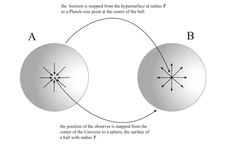
Figure 11: The ball A represents the universe as it appears to us, located at the center and observing a space-time extended in any direction (solid angle 4$\pi$) up to the horizon at distance $\cal T$. The arrows show the direction of light from the horizon to us. Ball B on the right represents instead the “dual” situation, with the horizon, corresponding to the origin of space-time, at the center, and the light rays, indicated by the arrows, propagating this time outwards. We are sitting on a point on the surface, a two-sphere oriented inwards. The curvature therefore is negative. This surface has to be thought as an “ideal” surface: different points on the surface belong to different causal regions: there is no communication among them. The only point of it we know to really exist is the one at which we are located. From a “real” point of view, the two-sphere boundary of ball B is therefore a “class of surfaces”, in each of which all the points of the surface have to be though to correspond to a single point in the “real” space-time. The path of light rays is therefore not straight but curved. Figure 12 helps to figure out the situation. Both figures should be taken in any case only as a hint, none of them being able to depict the exact situation.

In order to help the reader in visualizing the situation, we show in figure 12 a two-dimensional, intuitive picture of the universe, illustrating the fact that, both for a flat and a curved space-time, incident light rays arrive parallel to the hyperplane tangent to the observer, so that no difference is in practice locally observable (the only indication that the path of light is not straight but curved comes from a measurement of the cosmological constant or of a non-vanishing contribution to the stress-energy tensor). Owing to the curvature of space-time, the rays don’t come from the apparent horizon, the one obtained by straightly continuing the light paths along the tangent plane, but from a ”point-like” horizon.

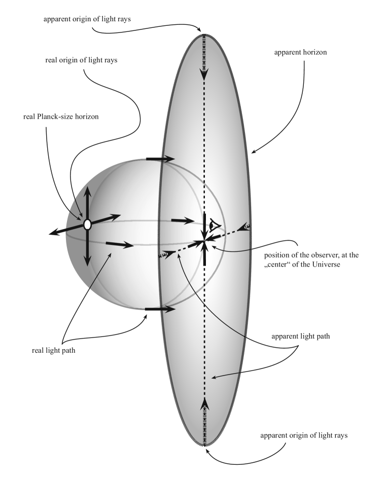
Figure 12: The disc represents the space-time as it appears to the observer: a flat, tangent space. The real space-time is however curved: the border of the disc corresponds to a “point” on a 3-sphere, and is located diametrically to the position of the observer.

Although useful to the purpose of illustrating how things are going, both figures 11 and 12 are slightly misleading, none of them being able to account for the real situation. In particular, from figure 11 we understand that there is a symmetry between picture A on the left and picture B on the right. Mapping from A to B, i.e. exchanging the origin with the horizon, involves a “time inversion”. This operation corresponds to a duality of the system. The configuration “B”, associated to the solution 7.106 of the Einstein’s equations, corresponds to one of the possible points of view, “pictures”, from which to look at the problem. Had we looked from the seemingly rather unnatural picture A, we would have concluded that the curvature is positive. However, this too is a legitimate point of view.

Let’s have a closer look at the situation we are describing. As seen from the point of view of the origin of the universe, the “surface” given by the equation $x_{1}^{2}+x_{2}^{2}+x_{3}^{2}={\cal T}^{2}$ consists of points lying on non causally-related regions. We are sitting on a point of this surface, which however is an “ideal” surface: the only point we know to exist is the one at which we are sitting, the hypothesis of boundedness of space-time being precisely justified by the requirement of describing only the region causally connected to us (alternatively, we can think that this surface must be thought as equivalent to a point). In general, our universe is the set of points, each one lying on a sphere $x_{1}^{2}+x_{2}^{2}+x_{3}^{2}=r^{2}\,<{\cal T}^{2}$, causally connected to us (notice that any 2-sphere with radius $r<{\cal T}$ contains several points causally connected to us). The curvature experienced by the observer is positive: from the point of view of the observer such a space made of a staple of two-spheric shells can be seen as obtained by starting from two-sphere corresponding to the surface at the horizon, and stapling two-spheres progressively more and more shrunk, till the one he is sitting on, which is shrunk to a point. In other words, the space “opens up” from the point of the observer, as roughly illustrated in figure 13. If we consider the region causally connected to us as the only one we indeed know to exist (and therefore have the right to consider), and therefore as the full existing space-time, it happens that the light rays starting from a “point”, the origin of the universe, end up also to a point, our point of observation. It is not hard to realize that what we are describing is indeed the geometry of a 3-sphere.

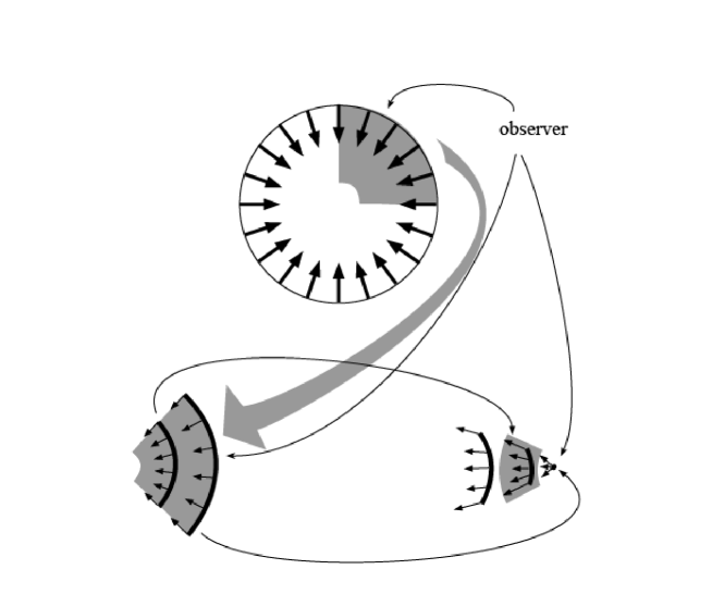
Figure 13: Shrinking to a point the two-sphere on which the observer is located (here represented by the external boundary of the disk), and considering the region causally connected to it, leads to a 3-sphere geometry and to a change of sign of the curvature.

The curvature of a 3-sphere is three times larger than the one of a two-sphere with the same radius. This means that, from a classical point of view, only one third of the whole curvature of the universe is of purely ”geometric” origin. Indeed, what we have investigated here is the pure ”cosmological” contribution to the energy density of the universe. The missing part can be explained within the framework of a quantum scenario, such as the string scenario we discuss in Ref. [1] (see also Ref. [2]). We refer to [1], section 3.1, for a discussion of the other contributions to the curvature of the universe.

7.5 Closed geometry, horizon and boundary

We want now to see how our universe builds up according to the combinatorial scenario of section 2. At $t=1$ there is only one possible configuration, that we illustrate in figure 14 with a ball representing the unit cell.

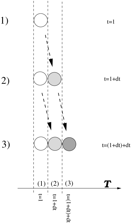
Figure 14: The progress of the universe through increasing times $\sim$ number of elementary cells. As the statistics grows, the configuration gets more complex and differentiated. Configuration 3) does not “include” configuration 2), which in turn does not include number 1): with volume increases also the radius, and the curvature of space decreases. The curvature and therefore the energy levels are different at different times. Configuration 1) “flows” to 2), and 2) to 3) only in the sense that 2) is more similar to 3) than 1) or a configuration with two equal balls are, and therefore this is the most realized “evolutionary path”.

Already at the next step, $N=2$, we have many more (infinitely many) possibilities, corresponding to any possible space “dimension”, being $N^{p}$ no more trivial, and the combinatorics increases very rapidly. For what discussed in section 2.2 we can concentrate the analysis to three dimensions, which gives a contribution of the same amount as the sum of all the neglected dimensionalities and configurations (Uncertainty Principle). The dominant configuration is the one that gives a “homogeneous” distribution of the occupied cells (what at large $N$ becomes a “spheric” geometry) . But already at $N=2$ also non-extremal entropy configurations start to exist and give non-trivial contributions. The result is that, on the top of a homogeneous distributions, in the universe start to show up inhomogeneities, of the order of the Uncertainty Relations. We can represent this process by distinguishing the regions of the space as balls with a different colour, figure 14. As time goes by (i.e. $N$ increases), we get new possibilities of differentiation from the basic homogeneity, in a sort of “progressive differentiation through steps of small perturbations”. We indicate this with an increasingly darker coloration of the balls. In principle, one could ask if there could be “discontinuities” in this progress, namely, whether there could be steps in which a darker ball falls between lighter balls, as illustrated in figure 15.

Figure 15: Configuration B) is obtained by superposing to the dominant configuration less entropic configurations than in A), and therefore has a lower weight, the more and more negligible the higher is the “jump” between B) and A).

Of course, nothing prevents these configurations from appearing, and indeed they are present. However, they are less entropic than ”smoother” ones: the entropy of a configuration decreases the more and more, the more it deviates from the ”regular” geometry of the sphere. Configuration presenting discontinuities give therefore a minor contribution, so that, in the average, the evolution takes place in the continuous way we illustrate in figure 17.

The progress through times/values of the average curvature and its inhomogeneities looks therefore like the propagation of a perturbation, and is translated, in the continuous language, into a “propagation” of the information through an expanding universe. As time goes by, the average curvature of space decreases, and this takes place everywhere, throughout all the space. The “perturbations” too spread out: as $1/N^{2}$ for those that we interpret as “massless fields”, or with a lower rate for the “massive” ones. To an observer, the local physics appears to be influenced, “produced” if one prefers, by the sum of the information that propagated up to him from everywhere else in the space. We already mentioned that a detector is a particular configuration of space, and an experiment is the detection of variations of this configuration during a certain interval of time. By letting an experiment, or a detection, to take place in a certain interval of time, the observer can resolve for different “smearing rates” of the inhomogeneities, and consequently organize the interpretation of what happens in terms of massless and/or massive objects. Of course, this is only an approximation, because any possible configuration contributes, although to an uncertainty expressed by the Uncertainty Principle. The “experimental observation” of the universe surrounding an observer indeed carries the information about the geometry of the full universe, the progress toward an increasing “local” differentiation from the average geometry being interpretable as a continuous, “jump-less” evolution that propagates the perturbation of the spheric geometry. What we observe is indeed always just our local physics, but we disentangle the jungle of data by organizing them as a superposition of informations coming from different places, and therefore “originating” at different times in the past. Notice that, although we see regions of the universe corresponding to past times, we don’t see ourselves in our past times: neighboring shells are not derived the one from the other through time evolution.

At any time ${\cal T}$ the universe is given by the (weighted) superposition of the configurations of the phase space at present time.

In this sense, the actual configuration depends only on the present phase space, not on the past: the evolution belongs to our interpretation. For the observer the universe turns out to mainly consist of a progression from the farthest configuration, the “initial” one, to the nearest, representing the physics at present time. At any time, the dominant configuration is however not derived by a process of evolution of the one at previous time.

Figure 16: During the time evolution, the three-dimensional space build up of an increasing number of elementary cells expands with the geometry of a three-sphere of growing radius.

To an observer the space appears built as an “onion”: the observer is surrounded by shells, two-spheres corresponding to farther and older phases of the universe, up to the horizon, that correspond to the “big bang”, as illustrated in figure 17.

Figure 17: The universe at time ${\cal T}$ appears to the observer as a set of surrounding shells made out of elementary cells. These shells, here represented only through sections constituted by two linked antipodal cells, go from the one closest to the observer (the darkest one), which is also the closets in time, up to the farthest, the horizon, that corresponds to the “big-bang” cell. The curvature of space is on the other hand everywhere the one of the age corresponding to the observer, ${\cal R}\sim 1/{\cal T}^{2}$. Notice that the two-sphere corresponding to the horizon appears to “conserve” the total energy flux, $1$, of the initial unit cell.

However, in itself there is no real “big-bang point”, located somewhere in this space: the argument leading to this description of the observed universe is not related to a particular choice of the point of observation. This does not mean that the universe looks absolutely identical for any choice of this point inside the whole space; simply, it means that from any point the universe appears built as an “onion”, with informations coming from everywhere around, going backwards in time, and space, up to the horizon, which is an “apparent horizon”, with no real physical location, but always at distance $N\sim{\cal T}$ from the observer.

Wherever the location of the observer in the space is, what he will see is only the “tangent” space around him, experienced through the modifications it produces in himself. In this way, he will have access to the knowledge of the average energy density of the universe, and indeed an indirect experience of the whole universe: the “local physics” is the one specific of the actual time, and as such “knows” about the full extension of the space. Owing to the special “boundary conditions” that “sew” the borders of space into a sphere, the latter will look in the average homogeneous all around in every direction: the observer will always have the impression of being located “at the center” of the universe. Through the modification of his configuration, the “local physics”, (i.e. the set of all what happens to him, light rays hitting from the various directions, gravitational fields etc…, that he will interpret as coming from all over the space around), he will then “measure” the energy density through all the space, concluding that it is $\rho(E)\sim 1/R^{2}$. On the other hand, knowing that such an energy-density scaling law is the one of a sphere, he will deduce that the horizon surface at a distance $R$ from himself, and with area $\sim R^{2}$, has boundary conditions such that the space closes-up to a sphere. The observer will then interpret the set of cells spread out along the horizon, a surface with area $\sim R^{2}$ and energy density $\sim 1/R^{2}$, as corresponding to a point, a unique cell of unit volume and unit energy, “smeared” over something that appears like a two-sphere. He will therefore refer to this as to the “Big Bang” point, the initial configuration, energy one at volume one, and he will say that what he sees by looking at the horizon, is indeed the beginning of everything. We repeat however that this point, or surface, namely, the horizon, does not really exist as a special point located somewhere in space: the interpretation would be the same for any observer, located at whatever point in this space.

7.6 Quantum geometry

If one divides the total energy of a Schwarzschild black hole, as given by the relation $2M=R$, by the volume of the three-ball enclosed by the two-sphere surface of the horizon, i.e. by ${4\over 3}\pi R^{3}$, one finds an energy density which, once inserted into the Einstein’s equation relating the curvature of space to the energy-momentum tensor, precisely corresponds to the curvature of a three-sphere. So, one starts with an object that from outside looks like a ball, i.e. a flat space, and finds out that ”as seen from inside” looks like a sphere, a curved space. This is the situation of our universe: despite the fact that a sphere doesn’t have boundary, as observers located inside we have the impression that there indeed is a surface, a two-sphere at radius $R$, the natural boundary of the universe, which works as the horizon of a black hole. In the discussion of the previous sections, we have seen that the topology of this boundary is however very special: as a matter of fact, it is the expanded representation of just a point. From the point of view of classical geometry, being the universe a sphere and being the interior of a black hole are conditions that cannot be both consistent at the same time. The point is that the true geometry of the universe is a quantum geometry. From the discussion of section 5.5. One can see that, close to the horizon of a black hole, the metric is heavily affected by the contribution of configurations of lower entropy. These are the less classical ones, the ones with a higher quantum delocalization. Going closer and closer to the horizon, the quantum non-localization increases, and at the limit of the ”point” of big bang, the non-localization is the maximal one: this point covers the entire horizon of the universe (see discussion in Ref. [6]).

7.7 Non-locality and quantum paradoxes

The uncertainty encoded in the Uncertainty Principle, lifting up the predictive power of classical mechanics to a probabilistic one, leads also to non-locality, possibly violating the bound on the speed of transfer of information set by the speed of light $c$.

It has been a long debated question, whether this had to be considered as something really built-in in natural phenomena, or simply an effect due to our ignorance of all the degrees of freedom involved, something that could be explained through the introduction of “hidden variables” [18]. It seems that indeed the physical world lies on the side of true quantum interpretation, which, as shown by Bell [19], is not reproducible with hidden variables. At the quantum level, the bound on the speed of information, $c$, can be violated by non-locality of wave-functions. How can we understand all that in the light of our framework? In our framework, the uncertainty of the Uncertainty Principle, at the base of quantum mechanics, is due to the fact that what we observe and measure is the sum of an infinite number of configurations, among which also tachyonic ones contribute. This is in agreement with the fact that non-locality implies somehow a propagation at speed higher than $c$, thereby violating causality. And indeed, the “dynamics” described in the previous section, resulting from the fact that at any time the universe is the sum of all configurations at the actual time, implies in some sense an instantaneous transfer of information: although the classical geometric deformations propagate at maximal speed $c$, the local configuration around the observer is uniquely related to the whole configuration of the universe. At any time, an electron, or any other particle, “knows” how large is the universe up to the horizon. How would such a boundary information determine the properties of each particle, even those locally produced in laboratory, if any information could only be transferred at maximal speed $c$? This non-local, basically instantaneous knowledge implied in the combinatoric scenario is reproduced in string theory, a relativistic theory, essentially in two ways:

1) through an explicit quantization, imposed in order to reproduce the ordinary quantum effects, which include non-local, tachyon-like effects such as experiment correlations violating Bell’s inequalities and so on, and

2) through the very basic properties of the string construction, in which, as we discuss in [1] (see also Ref. [2]), massive particles live partly in the extended space, identified with the ordinary space-time, the space along which they propagate, and partly have a foot in the internal string space.

Roughly speaking, being extended also in the internal space provides massive states an extra dimension from which they can “look” at the entire space-time, anyway a compact space, of which they can “see” the boundary, because the internal coordinate is non-local with respect to the external ones (see figure 18).

Figure 18: A pictorial illustration of how can massive particle/fields have knowledge of the full space-time. Here the extended but compact space-time is represented as a disc on the horizontal plane. The internal dimension is represented by the vertical segment. A field/particle confined to live tangent to the space-time cannot “see” the horizon, but just the neighborhoods of the point where it is sitting. A particle/field with a foot on the internal space can lift-up its point of view and see the horizon, having from above a global view of the disc on the plane.

This is not true for the massless fields (photon and graviton), that live entirely in the extended space-time. They therefore feel only the local physics.

7.8 The role of T-duality and the gravitational coupling as the self-dual scale

T-duality acts in string theory in such a way to ensure the existence of extra matter and fields, in the right amount to imply the presence of both a strongly and a weakly coupled sector. It is the presence of both these sectors what stabilizes the scale: if there was just one of the two, we would be no scale at all, because both the gravitational and the interaction scale would become ”running” scales”. In our framework, gravitational interactions are the characterization at the level of vectorial representation of space of the evolution through “geometries” of energies. When introducing the investigation of the deformations of the dominant geometry in terms of propagating fields and particles, we said that the finest description of the three-dimensional sphere is not vectorial, but spinorial. One would have the impression that a spinorial space is a better environment in which to investigate the geometries of the distribution of energies, already at the level of the discussion of section 2.2. Indeed, deformations of the main geometry as given by spinor fields weight less, and as such can be treated as perturbations, “quantum perturbations”. This is basically the reason why we perceive a space which is classically a vector space. Spinors (which in our framework are only matter particles) turn out to come in the game with the role of describing objects, “energy packets” which move at lower speed than the expansion of the classical space, and the propagation of information, itself. Gravity is the ”average” interaction, the one related to the measure, and scale, of space, intended as the average geometry resulting from all the contributions to energy given also by the other interactions. Its coupling is therefore ”in between” strong and weak coupling, and is set to 1 by convention (one may take this as a renormalization prescription). If all the interactions were ”weak”, the space would be only spinorial (we would perceive the space as spinorial, therefore we would not see propagation of information through vectorial bosons). It is the existence of both weakly and strongly coupled sectors (consequence of, even softly broken, T-duality) what forces spinors to behave also as vectors, and results in an impression of vectorial geometry of space.

7.9 Natural or real numbers?

In this work, we have introduced an interpretation of the real world as the collection of all possible “binary codes”. The universe mostly appears as the average of these configurations, that we interpret as assignments of energy amounts along a space. Reducing everything to a collection of binary codes means reducing everything to a discrete description in terms of natural numbers. One may ask the question: are natural numbers enough to encode all the information of the universe, or is there a finer description, for instance in terms of real numbers? Are we sure that with natural numbers we can catch, and express, all the information? At first sight, one would say that real numbers say “more”, allow to express more information. Moreover, they appear to be “real” in the true sense of something existing in nature. For instance, one can think to draw with the pencil a circle and a diameter. Then, one has physically realized two lines of lengths that don’t stay in a ratio expressible as a rational number. However here the point is: what is really about the microscopical nature of these two drawings? At the microscopical level, at the scale of the Planck length, the notion of space itself is so fuzzy to be practically lost. In our scenario, an analysis of the superposition of configurations tells us that, before reaching this scale, remote configurations, whose contribution is usually collected under the Heisenberg’s Uncertainty, count more and more. In other terms, the world is no more classical but deeply quantum mechanical, to the point that the uncertainty in the length of the two lines doesn’t allow us to know whether their ratio is a real or a rational number. Moreover, real numbers are introduced in mathematics through procedures, such as limits, Dedekind sections etc., whose informational content can be “written” as a text with a computer program, such as the one with which I am writing here these words. This means that, as a matter of pure information, real numbers can be introduced via natural numbers. Perhaps, all the information of the universe is expressible through natural numbers, and, as a consequence, the discrete description of the universe, and in particular of space-time, is not just a simplification, an approximation, but indeed the most fundamental one can think about.

References

- [1] A. Gregori, Combinatorics, observables, and String Theory, part II (2011).
- [2] A. Gregori, An entropy-weighted sum over non-perturbative vacua, arXiv:0705.1130 [hep-th].
- [3] A. Gregori, About combinatorics, and observables, arXiv:0712.0471 [hep-th].
- [4] A. Gregori, Relativity as classical limit in a combinatorial scenario, arXiv:0911.0518v1 [physics.gen-ph].
- [5] A. Gregori, On the Critical Temperatures of Superconductors: a Quantum Gravity Approach, arXiv e-prints (July, 2010) arXiv:1007.3731.
- [6] A. Gregori, Is the Universe the only existing Black Hole?, ArXiv e-prints (June, 2010) 1006.5826.
- [7] A. Gregori, A note on the phases of natural evolution, arXiv:0712.0074 [physics.gen-ph].
- [8] M. Rabinowitz, n-dimensional gravity: Little black holes, dark matter, and ball lightning, Int. J. Theor. Phys. 40 (2001) 875–901, astro-ph/0104026.
- [9] A. Gregori, Entropy, string theory, and our world, hep-th/0207195.
- [10] A. Gregori, Naturally time dependent cosmological constant in string theory, hep-th/0402126.
- [11] J. M. Bardeen, B. Carter, and S. W. Hawking, The Four laws of black hole mechanics, Commun. Math. Phys. 31 (1973) 161–170.
- [12] J. D. Bekenstein, Black holes and entropy, Phys. Rev. D7 (1973) 2333–2346.
- [13] L. D. Landau and E. M. Lifshitz, The Classical Theory of Fields.
- [14] C. Vafa, Evidence for F-Theory, Nucl. Phys. B469 (1996) 403–418, hep-th/9602022.
- [15] J. Wess and J. Bagger, Supersymmetry and Supergravity, ch. I. Princeton University Press, 1992.
- [16] A. Sagnotti, Open strings and their symmetry groups, hep-th/0208020.
- [17] E. Kiritsis, Introduction to superstring theory, hep-th/9709062.
- [18] A. Einstein, B. Podolsky, and N. Rosen, Can Quantum Mechanical Description of Physical Reality Be Considered Complete?, Phys. Rev. 47 (May 15, 1935).
- [19] J. S. Bell, On the Einstein Podolsky Rosen Paradox, Physics 1 (1964) 195–200.