Bell inequalities as constraints on unmeasurable correlations

Abstract

The interpretation of the violation of Bell-Clauser-Horne inequalities is revisited, in relation with the notion of extension of QM predictions to unmeasurable correlations. Such extensions are compatible with QM predictions in many cases, in particular for observables with compatibility relations described by tree graphs. This implies classical representability of any set of correlations $\langle A_{i}\rangle$, $\langle B\rangle$, $\langle A_{i}B\rangle$, and the equivalence of the Bell-Clauser-Horne inequalities to a non void intersection between the ranges of values for the unmeasurable correlation $\langle A_{1}A_{2}\rangle$ associated to different choices for $B$. The same analysis applies to the Hardy model and to the “perfect correlations” discussed by Greenberger, Horne, Shimony and Zeilinger. In all the cases, the dependence of an unmeasurable correlation on a set of variables allowing for a classical representation is the only basis for arguments about violations of locality and causality.

Introduction and results

The implications of the violation of Bell inequalities [1] in Quantum Mechanics (QM) are still controversial. On one side, their logical and probabilistic nature has been recognized and discussed [2], [3], [4] and their fundamental meaning traced back [5] to Boole’s general notion of conditions of possible experience [6]. In this perspective, their violation, which excludes representability of quantum mechanical predictions by a classical probability theory, shows general and fundamental differences between the classical and the quantum notion of event.

On the other, the violation of Bell inequalities is interpreted by many authors in terms of “non local properties” of QM; an extensive review of such positions is contained in Ref. [7] and a discussion of their basic logical steps is in Refs. [8], [9], [10], [11].

In our opinion, in general, the use of Bell inequalities for the analysis of QM and of its interpretation is in a sense incomplete because their violations simply amounts to a negative result, i.e. the inconsistency between QM and the whole set of assumptions entering in their derivation.

The present paper is an attempt to reconsider the situation from a more constructive point of view, beginning with QM predictions, trying to represent them by classical probability models in a sequence of steps and asking which step may fail.

We recall that adopting a classical probability model exactly amounts to assuming that all variables together take definite, even if possibly unmeasurable, values, with definite probabilities.

Since a classical probability model is equivalent to its set of predictions for all correlations, while QM only predicts correlations between compatible observables, classical representability also amounts to an extension of QM predictions to unmeasurable correlations, e.g., correlations between two components of the spin of the same particle, or polarization of the same photon along different directions.

A central role is therefore played by the notion of extension of QM predictions to unmeasurable correlations. We shall use basic and general constraints on such extensions to discuss the violation of Bell inequalities in terms of actual properties of existing (partial) extensions rather than in terms of incompatibility between assumed principles. In particular, this will allow for a definite answer to the question what precisely is “influenced” in arguments on non-local effects in QM.

The extension problem outlined above has been studied in general in [12]. One of the result (see Sect.1) is that classical representability always holds for yes/no observables with compatibility relations described by a tree graph, i.e. a graph in which any two points are connected by exactly one path, with points representing observables and links predicted correlations.

In the case of four yes/no observables, $A_{1},A_{2},B_{1},B_{2}$, $A_{i}$ compatible with $B_{j}$, this implies that, for fixed $B$, any pair of probabilities for the subsystems $A_{i},B$ $i=1,2$, assigning the same probability to the outcomes of $B$, admits extensions to a probability on the whole system $A_{1},A_{2},B$, each giving a definite value to the possibly unmeasurable correlation $\langle A_{1}A_{2}\rangle$. As we will see, the results on tree graphs also imply that if a value can be assigned to $\langle A_{1}A_{2}\rangle$ consistent with two choices $B_{1}$, $B_{2}$ for $B$, then the whole system $A_{i},B_{j}$ admits a classical representation.

Since the converse is obvious, it follows that the existence of a classical representation for given set of expectations $\langle A_{i}\rangle$, $\langle B_{i}\rangle$ and correlations $\langle A_{i}B_{j}\rangle$ is equivalent to the possibility of giving a value to $\langle A_{1}A_{2}\rangle$ which is consistent with the two choices for $B$.

The analysis of QM models with four yes/no observables is therefore reduced in general to the consistency (i.e. a non void intersection) between the ranges of the (hypotetical, unmeasurable) values for the correlation $\langle A_{1}A_{2}\rangle$ allowed by (measurable) given correlations of $A_{1}$ and $A_{2}$ with $B_{1}$ and $B_{2}$.

With respect to the same conclusion obtained by Fine [2], we stress that probabilistic descriptions of three-observable subsystem automatically exist and only their compatibility is in question; moreover, only a repeated application of the results for tree graphs is required by our argument.

In Sect.2 , the possible range for $\langle A_{1}A_{2}\rangle$, depending on the measurable correlations $\langle A_{i}B\rangle$, is characterized in terms of elementary three-observable inequalities. QM states which violate Bell inequalities are shown to give rise to disjoint intervals for the admissible values of $\langle A_{1}A_{2}\rangle$ in automatically existing probabilistic models for $A_{1},A_{2},B_{1}$ and $A_{1},A_{2},B_{2}$. This clearly shows that classical representability of such states exactly fails in the attribution of a value to an unmeasurable correlation.

Actually, since BCH inequalities, more precisely, the eight inequalities discussed by Fine [2], are equivalent to classical representability, their violation exactly amounts to the inconsistency of such an attribution.

The same discussion and result apply to the states introduced, on the same set of observables, by Hardy [8] and exploited in Stapp’s work [9], discussed by Mermin [10]. In particular, Stapp’s and Mermin’s discussion exactly concerns partial extensions and the origin of the inconsistency of the ranges of value for an unmeasurable correlation $\langle A_{1}A_{2}\rangle$ associated as above to the correlations of $A_{i}$ with $B_{1}$ and $B_{2}$ respectively.

In Sect.3, the experiment proposed by Greenberger, Horne, Shimony and Zeilinger (GHSZ) [13] is analyzed along the same lines. The QM correlations defined by the GHSZ state, between observables $A_{i}$, $B_{i}$, $C_{i}$, $i=1,2$, are shown to extend to all correlations within the sets of observables $A_{i},B_{i},C_{1}$ and $A_{i},B_{i},C_{2}$; both extensions give unique values for an unmeasurable correlation, $\langle A_{1}A_{2}B_{1}B_{2}\rangle=\pm 1$, and the sign depends on the choice between $C_{1}$ and $C_{2}$. Again, only the attribution of a value to an unmeasurable correlation depends on the choice of an additional observable.

In the last Section we will comment on the fact that such a dependence is the only basis for arguments about non local and non causal effects.

1 Extensions of QM predictions

A basic notion is that of yes/no observables, denoting physical devices producing, in each measurement, i.e. in each application to a physical system, two possible outcomes; by experimental setting we will denote a collection of yes/no observables.

Within an experimental setting, an (experimental) context will denote a (finite) set of observables which “can be measured together on the same physical system”, in the precise sense that their joint application to a physical system gives rise to a statistics of their joint outcomes given by a classical probability, i.e., by a normalized measure on the Boolean algebra freely generated by them. Observables appearing together in some context will be called compatible; their correlations will be called measurable, or observable.

In the following, Quantum Mechanics will be interpreted as a theory predicting probabilities associated to experimental contexts defined by sets of commuting projections. Joint statistics of non compatible observables are not defined in the above setting; correlations between incompatible observables will be called unmeasurable, or unobservable.

In particular, we will consider the Bell-Clauser-Horne (BCH) experimental setting, consisting of two pairs ($A_{1}$, $A_{2}$), ($B_{1}$, $B_{2}$), of incompatible yes/no observables, taking values in $\{0,1\}$; the $A_{i}$ are compatible with the $B_{j}$, i.e. they can be measured together, in the sense introduced above. Such variables may be interpreted in terms of spin components or photon polarizations, each pair referring to one of a pair of particles, possibly in space-like separated regions.

The experimental contexts given by QM consist, in the BCH setting, of the four pairs $\{A_{i},B_{j}\}$; probabilities are associated to contexts, see Proposition 1.3 below, by the observed relative frequencies $\langle A_{i}\rangle$, $\langle B_{j}\rangle$, and $\langle A_{i}B_{j}\rangle$. QM predictions for the BCH setting precisely consist in probabilities on contexts, given by the spectral representation for the corresponding sets of commuting projectors.

Such a partial nature of QM predictions is a very general fact since the (ordinary) interpretation of QM precisely consists of a set of probability measures, each defined, by the spectral theorem, on the spectrum of a commutative subalgebra of operators in a Hilbert space. Such a structure has been formalized in [12] as a partial probability theory on a partial Boolean algebra.

A basic problem for the interpretation of QM is the necessity of such partial structures; in other words, whether they admit a classical representation, i.e. common probabilistic classical description in a probability space $(X,\Sigma,\mu)$, where $X$ is a set, $\Sigma$ a $\sigma$-algebra of measurable (with respect to $\mu$) subsets and $\mu$ is a probability measure on $X$ and all (yes/no) variables are described by characteristic functions of measurable subsets. Clearly, such a notion covers all kinds of “hidden variables” theories, all ending in the attribution of values to all the observables, with definite probabilities.

Extensions have been discussed in general in [12]. Non trivial extensions, describing QM predictions through a reduced number of contexts, have been shown to arise in some generality and some of the results can be described in terms of graphs:

Proposition 1.1.

Consider any set of probabilities $p_{i}$ on a set of yes/no observables $A_{i}$ and correlations $p_{ij}$ on a subset of pairs $A_{i},A_{j}$, defining a probability on each pair $A_{i},A_{j}$, with $p_{i}=\langle A_{i}\rangle$, $p_{j}=\langle A_{j}\rangle$, $p_{ij}=\langle A_{i}A_{j}\rangle$; describing observables $A_{i}$ as points and the above pairs as links in a graph, any subset of predictions associated to a tree subgraph admits a classical representation.

Proposition 1.2.

the same holds with yes/no observables $A_{i}$ substituted by free Boolean algebras $\mathcal{A}_{i}$, $p_{i}$ by probabilities on $\mathcal{A}_{i}$, $p_{ij}$ by probabilities on the Boolean algebra freely generated by the union of the sets of generators of $\mathcal{A}_{i}$ and $\mathcal{A}_{j}$.

Propositions 1.1 and 1.2 are proven in [12] by induction on the number of links of the correlation tree, by an explicit construction of a probability on the Boolean algebra generated by two algebras in terms of conditional probabilities with respect to their intersection. The resulting probabilities are in general not unique.

The above Propositions can be interpreted as providing automatic conditions for the realization of the possibility advocated by Einstein, Podolsky and Rosen [14] to attribute a value to correlations between incompatible observables consistently with the QM predictions for the remaining, measurable, correlations; actually, they do not make reference to QM and give conditions on compatibility relations allowing the extension of any set of predictions.

It is also useful to recall the following elementary fact [12], which implies that it is sufficient to analyze correlations since they completely define a probability measure.

Proposition 1.3.

In a classical representation for $n$ observables $A_{1},\ldots,A_{n}$, the probability measure is completely defined by all expectation values $\langle A_{i}\rangle$ together with all possible correlations $\langle A_{i}A_{j}\rangle$, $\langle A_{i}A_{j}A_{k}\rangle$,…, $\langle A_{1}\ldots A_{n}\rangle$.

In the BCH setting, the two subsets $\{A_{1},A_{2},B_{1}\}$, $\{A_{1},A_{2},B_{2}\}$, with the correlations $\langle A_{j}B_{i}\rangle$ $j=1,2,$ are described by tree graphs (see Fig.1 (a),(b)) and admit therefore classical representations. It follows that all QM predictions can be reproduced by a pair of classical probability theories, one for the Boolean algebra freely generated by $A_{1},A_{2},B_{1}$ the other for $A_{1},A_{2},B_{2}$; both sets of variables include $A_{1}$ and $A_{2}$ and give rise to predictions for the unmeasurable correlation $\langle A_{1}A_{2}\rangle$.

In other terms, given a choice for $B$, one may consistently speak of the correlation $\langle A_{1}A_{2}\rangle$. Clearly, the existence of a classical representation for all the predictions in the BCH setting implies the existence of a value for $\langle A_{1}A_{2}\rangle$ compatible with the different choices of $B$.

On the other hand, if it is possible to give a value to $\langle A_{1}A_{2}\rangle$ independently of the choice $B_{1}$, $B_{2}$ for $B$, this defines, by Proposition 1.3, a probability on the Boolean algebra $\mathcal{A}_{12}$ generated by $A_{1},A_{2}$; then, the application of Proposition 1.2 to $\mathcal{A}_{12}$, $\{B_{1}\}$, $\{B_{2}\}$ implies classical representability of all the predictions for the BCH setting (see Fig.1 (c)).

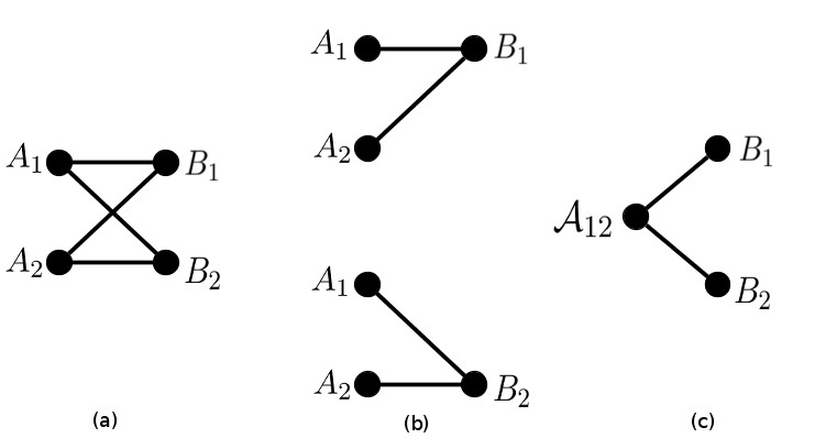
Figure 1: (a) BCH compatibility graph; (b) two tree subgraphs; (c) tree graph corresponding to extension of the measure on the algebra generated by $A_{1},A_{2}$

Classical representability and BCH inequalities (in the sense of Ref.[2]) are therefore equivalent to the possibility of attributing a common value to the unmeasurable correlation $\langle A_{1}A_{2}\rangle$ in classical models for $A_{1},A_{2},B_{1}$ and $A_{1},A_{2},B_{2}$.

In the next Section, we shall compute explicitly the range of $\langle A_{1}A_{2}\rangle$ allowed by the QM predictions for a pair of spin variables, in the zero total angular momentum state and for the state introduce by Hardy [8].

2 Explicit Constraints for systems of three and four observables

In this section we first recall simple constraints, for three $\{0,1\}$ valued random variables $A_{1},A_{2},B$, satisfied by $\langle A_{1}A_{2}\rangle$ given $\langle A_{i}\rangle$, $\langle B\rangle$ and $\langle A_{i}B\rangle$. We then show that, for the predictions given by both the QM states discussed by Bell and Hardy [8], such constraints give rise, for different choices of $B$, to incompatible values for $\langle A_{1}A_{2}\rangle$.

The possible ranges of correlations in a classical model for $\{A_{1},A_{2},B\}$ are given by the Bell-Wigner polytope [4], also discussed in [12]. We only need a subset of the corresponding set of inequalities, namely

$$0\leq\langle A_{1}A_{2}\rangle\leq\langle A_{1}\rangle$$ (1)

$$\langle A_{1}B\rangle+\langle A_{2}B\rangle-\langle B\rangle\leq\langle A_{1}A_{2}\rangle\leq\langle A_{2}\rangle-\langle A_{2}B\rangle+\langle A_{1}B\rangle$$ (2)

$$\langle A_{1}\rangle+\langle A_{2}\rangle+\langle B\rangle-\langle A_{1}B\rangle-\langle A_{2}B\rangle-1\leq\langle A_{1}A_{2}\rangle$$ (3)

Eq. (1) is trivial; the first relation in eq. (2) immediately follows from $\langle(A_{1}-B)(A_{2}-B)\rangle\geq 0$, which holds since for $B=1$ both factors are non positive, for $B=0$ they are both non negative; moreover, the first relation in eq. (2) implies the second by interchanging $B$ and $A_{2}$ and eq. (3) by interchanging $B$ and $1-B$. The complete set of constraints [4] includes three additional inequalities; they are obtained from the above relations through the interchange of $A_{1}$ and $A_{2}$ and the substitution of $B$ with $1$ in eqs. (1), (2) (and are not relevant for our analysis).

The constraints given by eqs. (1), (2) (3), applied to QM predictions for mean values and observable correlations, may give rise to ranges of values for the unobservable correlation $\langle A_{1}A_{2}\rangle$ which are disjoint for different choices of $B$.

Consider in fact a system of two spin $1/2$ particles in the singlet state ${\frac{1}{\sqrt{2}}(\lvert+-\rangle-\lvert-+\rangle)}$ and associate $A_{1}$ and $A_{2}$ with the projectors on the spin up state along directions $\hat{x}$ and $\hat{z}$ for the first particle and $B_{1}$ with the projector on the spin down state along the direction $\frac{\hat{x}+\hat{z}}{\sqrt{2}}$ for the second particle, namely

$$\frac{1+\sigma_{x}}{2},\qquad\frac{1+\sigma_{z}}{2},\qquad\frac{1}{2}-\frac{\tau_{x}+\tau_{z}}{2\sqrt{2}},$$ (4)

where $\sigma_{i}$’s and $\tau_{i}$’s are Pauli matrices acting, respectively, on the first and on the second subsystem. Quantum mechanical predictions give

$$\langle A_{1}\rangle=\langle A_{2}\rangle=\langle B_{1}\rangle=\frac{1}{2}\ ,$$ (5)

$$\langle A_{1}B_{1}\rangle=\langle A_{2}B_{1}\rangle=\frac{1}{4}+\frac{\sqrt{2}}{8}\ ,$$ (6)

Denoting by $\langle\text{ }\rangle_{1}$ correlations in a probabilistic model for $\{A_{1},A_{2},B_{1}\}$ eqs. (1) and (2) give

$$\frac{1}{4}<\frac{\sqrt{2}}{4}\leq\langle A_{1}A_{2}\rangle_{1}\leq\frac{1}{2}\ .$$ (7)

If $B_{1}$ is substituted by $B_{2}$, representing the projector

$$\frac{1}{2}-\frac{\tau_{x}-\tau_{z}}{2\sqrt{2}}\ ,$$ (8)

QM predictions give $\langle B_{2}\rangle=\frac{1}{2}$ and

$$\langle A_{1}B_{2}\rangle=\frac{1}{4}+\frac{\sqrt{2}}{8}\ ,\quad\langle A_{2}B_{2}\rangle=\frac{1}{4}-\frac{\sqrt{2}}{8}\ .$$ (9)

Eqs. (1) and (2) then give, for the unmeasurable correlation $\langle\text{ }\rangle_{2}$ in probabilistic models for $\{A_{1},A_{2},B_{2}\}$

$$0\leq\langle A_{1}A_{2}\rangle_{2}\leq\frac{1}{2}-\frac{\sqrt{2}}{4}<\frac{1}{4}\ .$$ (10)

It follows that the value of $\langle A_{1}A_{2}\rangle$ must belong to one of two disjoint intervals, depending on whether one is considering the probability space for $\{A_{1},A_{2},B_{1}\}$ or that for $\{A_{1},A_{2},B_{2}\}$, i.e. whether one chooses to measure $B_{1}$ or $B_{2}$ on the second subsystem. Therefore, the validity of QM predictions for compatible observables does not allow to assign a definite value to the correlation $\langle A_{1}A_{2}\rangle$, independent of the choice of the measurement to be performed on the second subsystem.

The second example is Hardy’s experiment [8], also exploited in Stapp’s [9] and Mermin’s [10] discussion; we shall refer to Mermin’s notation. As in the previous example, we have two spin $1/2$ particles and four yes/no observables, denoted by $L1,L2$ and $R1,R2$, acting respectively on a “left” and a “right” particle. The state is described, up to a normalization factor, by the vector

$$\lvert\Psi\rangle=\lvert L1+,R1-\rangle-\lvert L2-,R2+\rangle\langle L2-,R2+\lvert L1+,R1-\rangle\ ,$$ (11)

where, e.g, $\lvert L1+,R1-\rangle$ indicates a simultaneous eigenstate of the commuting observables $L1$ and $R1$ with eigenvalue $1$ on the left and $-1$ on the right.

The variables $A_{i}$, $i=1,2$, are associated with the propositions “the result of the measurement of $Ri$ is $+1$”, the same for $B_{i}$ and $Li$; as before, $A_{i}$ and $B_{i}$ take values in $\{0,1\}$. Independently of the specific expressions for $Li$ and $Ri$, QM predicts the following correlations (corresponding to eqs.(6)-(9) in Ref. [10]):

$$1-\langle A_{2}\rangle-\langle B_{1}\rangle+\langle A_{2}B_{1}\rangle=0\ ,$$ (12)

$$\langle A_{2}\rangle-\langle A_{2}B_{2}\rangle=0\ ,$$ (13)

$$\langle A_{1}B_{2}\rangle=0\ ,$$ (14)

$$\langle A_{1}\rangle-\langle A_{1}B_{1}\rangle>0\ ,$$ (15)

In eq. (15), $>0$ is equivalent to $\neq 0$ in Ref. [10] since $\langle A_{1}\rangle\geq\langle A_{1}B_{1}\rangle$ always holds.

Eqs. (3), (12) and (15) give, in all classical models for $\{A_{1},A_{2},B_{1}\}$

$$\langle A_{1}A_{2}\rangle_{1}\geq\langle A_{1}\rangle+\langle A_{2}\rangle+\langle B_{1}\rangle-\langle A_{1}B_{1}\rangle-\langle A_{2}B_{1}\rangle-1=\langle A_{1}\rangle-\langle A_{1}B_{1}\rangle>0\ ;$$ (16)

on the other hand, in classical models for $\{A_{1},A_{2},B_{2}\}$, eqs. (2), (12) and (15) give,

$$\langle A_{1}A_{2}\rangle_{2}\leq\langle A_{2}\rangle-\langle A_{2}B_{2}\rangle+\langle A_{1}B_{2}\rangle=0\ ,$$ (17)

which also implies, by eq. (1),

$$\langle A_{1}A_{2}\rangle_{2}=0\ .$$ (18)

As in the previous example, no value for the unmeasurable correlation $\langle A_{1}A_{2}\rangle$ is compatible with different choices of $B_{i}$. A peculiarity of this case is that in classical models for $\{A_{1},A_{2},B_{2}\}$ the correlation $\langle A_{1}A_{2}\rangle$ is completely fixed (to $0$) by the constraints imposed by measurable correlations. Attributing the $0$ value is actually equivalent to asserting the logical implication $A_{1}\rightarrow A_{2}^{c}$, i.e. “if the measurement of $R1$ gives $+1$, then the measurement of $R2$ gives $-1$”; such an implication holds in all classical models for $\{A_{1},A_{2},B_{2}\}$ and fails in all classical models for $\{A_{1},A_{2},B_{1}\}$.

3 The perfect correlation model of GHSZ

In this Section, the above analysis is applied to the case considered in [13] and discussed in [15] within a general framework unifying Bell and Kochen-Specker kinds of results.

With a slight modification of the above terminology, the experimental setting involved in the GHSZ model consists of six yes/no observables, which can be described as $A_{i}$, $B_{i}$, $C_{i}$, $i=1,2$, taking values $1$ and $-1$; equivalently, by the propositions $P_{i}$, $Q_{i}$, $R_{i}$ respectively asserting $A_{i}=1$, $B_{i}=1$, $C_{i}=1$. The experimental contexts, i.e. the sets of compatible observables are given by the possible choices of (at most) one $A$, one $B$ and one $C$.

In Refs. [13] and [15] observables associated to different letters are interpreted as measured in distant, space-like separated regions. The above observables reproduce the example of Ref. [13], Sect. III, with the identification $A_{i}=A(\phi_{i})B(0)$, $B_{i}=C(\phi_{i})$, $C_{i}=D(\phi_{i})$, with $\phi_{1}=0$ $\phi_{2}=\pi/2$; in Mermin’s spin notation, they should be read as $A_{1}=-\sigma^{1}_{x}$, $A_{2}=-\sigma^{1}_{y}$, $B_{1}=\sigma^{2}_{y}$, $B_{2}=\sigma^{2}_{x}$, $C_{1}=\sigma^{3}_{y}$, $C_{2}=\sigma^{3}_{x}$.

In general, quantum mechanical predictions consist in probability assignments within each of the eight contexts defined by the choice of three indexes $i$; e.g. a context is given by the choice $A_{1}$, $B_{1}$, $C_{1}$, and the associated predictions by a probability on the Boolean algebra freely generated by the propositions $P_{1}$, $Q_{1}$, $R_{1}$.

The crucial point of GHSZ and Mermin’s analysis is the observation that, for suitable states, QM predictions give “perfect correlations” (each correlation involving observables in a fixed context), which are not compatible with any (context-independent) assignment of values to the variables $A_{i}$, $B_{i}$, $C_{i}$.

In fact, the state considered by GHSZ and Mermin can be written, for the Mermin spin variables $\sigma^{i}_{k}$, in the usual notation referring to the eigenvalues of $\sigma^{i}_{3}$,

$$\lvert\Psi\rangle=\frac{1}{\sqrt{2}}\ (\lvert+++\rangle-\lvert---\rangle)$$ (19)

and gives the correlations

$$\langle A_{1}B_{1}C_{1}\rangle=-1\ ,\qquad\langle A_{2}B_{2}C_{1}\rangle=-1\ ,$$ (20)

$$\langle A_{2}B_{1}C_{2}\rangle=-1\ ,\qquad\langle A_{1}B_{2}C_{2}\rangle=+1\ .$$ (21)

Values $a_{i},b_{i},c_{i}=\pm 1$ assigned to the above variables and reproducing the above correlations would satisfy the relations

$$a_{1}b_{1}c_{1}=-1\ ,\ \ a_{2}b_{2}c_{1}=-1\ ,\ \ a_{2}b_{1}c_{2}=-1\ ,\ \ a_{1}b_{2}c_{2}=+1\ ,$$ (22)

which have no solution since their product gives $1$ for the l.h.s., $-1$ for the r.h.s..

Following the program outlined above and using the notions and results of Sect. 1, we will extend the GHSZ and Mermin argument to show:

• the correlations eqs. (20), (21) and all the other QM predictions given by the GHSZ state, eq. (19), extend to classical probabilities $p_{1}$, $p_{2}$ on the two subsystems defined by $\{A_{1},A_{2},B_{1},B_{2},C_{1}\}$ and $\{A_{1},A_{2},B_{1},B_{2},C_{2}\}$

• unique and different values, $\pm 1$, are given by such $p_{1}$ and $p_{2}$ to the correlation $\langle A_{1}A_{2}B_{1}B_{2}\rangle$, all the other correlations between the $A$ and $B$ observables admitting common values;

• pairs of probabilities on the two subsystem introduced in $i)$ extend to a probability on the entire system generated by $A_{i},B_{j},C_{k}$, $i,j,k,=1,2$, exactly if they coincide on the subsystem generated by $A_{1},A_{2},B_{1},B_{2}$.

Again, the conclusion is that exactly a non observable correlation, $\langle A_{1}A_{2}B_{1}B_{2}\rangle$, depends on the choice of the observable $C_{i}$.

In order to derive $i)$ - $iii)$, we first observe that $iii)$ follows immediately from Proposition 1.2, applied to the Boolean algebra generated by $P_{i},Q_{j}$ and to its correlations with the observables $R_{1}$ and $R_{2}$, forming a tree graph.

Concerning $ii)$, observe that eqs. (20) imply, for any probabilistic model reproducing them, $A_{1}B_{1}C_{1}=-1$ and $A_{2}B_{2}C_{1}=-1$ with probability $1$, so that, with probability $1$, $A_{1}B_{1}A_{2}B_{2}=1$; equivalently, $\langle A_{1}B_{1}A_{2}B_{2}\rangle=1$. In the same way, eqs. (21) imply $\langle A_{1}B_{1}A_{2}B_{2}\rangle=-1$; such relations hold therefore for all probabilistic models reproducing, respectively, the QM correlations of the $A,B$ observables with $C_{1}$ and $C_{2}$. The existence of probabilities giving common values to all the other correlations follows from the construction below.

The most involved issue is $i)$, which is non trivial since quantum mechanical predictions involve eight different contexts and $i)$ states that the predictions given by the state (19) extend to all correlations between variables inside each one of only two contexts. Notice that Propositions 1.1 and 1.2 do not imply such an extension, since the corresponding set of correlations is not given by a tree graph and in fact not all quantum states admit it, as also implied by the BCH analysis; the exact form of the quantum predictions we are going to extend is therefore important. It is easy to see that the state given by eq. (19) gives rise to the correlations

$$\langle A_{i}\rangle=\langle B_{i}\rangle=\langle C_{i}\rangle=\langle A_{i}B_{j}\rangle=\langle A_{i}C_{j}\rangle=\langle B_{i}C_{j}\rangle=0\ ,\ i,j=1,2$$ (23)

$$\langle A_{1}B_{2}C_{1}\rangle=\langle A_{2}B_{1}C_{1}\rangle=\langle A_{2}B_{2}C_{2}\rangle=\langle A_{1}B_{1}C_{2}\rangle=0\ .$$ (24)

We have to show that the all the correlations given by eqs. (20),(21),(23),(24) involving the observables $A_{i},B_{j},C_{1}$ can be represented by a classical model, and the same for those involving $A_{i},B_{j},C_{2}$, and that the two models give the same correlations between variables $A_{i},B_{j}$ with the only exception of $\langle A_{1}A_{2}B_{1}B_{2}\rangle$.

The first classical model is defined as follows: let $A_{i},C_{1}$ denote variables taking values $1$ and $-1$ with probability $1/2$, i.e.

$$A_{i}^{2}=1\,,\ C_{1}^{2}=1\ ,\ \ \langle A_{i}\rangle=\langle C_{1}\rangle=0\ ,\ \ \langle A_{1}A_{2}\rangle=\langle A_{i}C_{1}\rangle=0$$ (25)

and define

$$B_{i}\equiv-A_{i}C_{1}\ .$$ (26)

Eqs. (25) and (26) immediately imply eqs. (20) and all eqs. (23),(24) not involving $C_{2}$.

The second model is defined in the same way, by independent variables $A_{i}$ and $C_{2}$ satisfying the same relations as in eqs. (25) and by variables $B_{i}$ now defined as

$$B_{1}\equiv-A_{2}C_{2}\ ,\ \ B_{2}\equiv A_{1}C_{2}\ .$$ (27)

Eqs. (21) and all eqs. (23), (24) not involving $C_{1}$ immediately follow.

All the correlations defined by the two models between $A$ and $B$ variables follow from eqs. (25), with $C_{2}$ replacing $C_{1}$ for the second model, (26),(27); in both models $\langle A_{1}A_{2}\rangle=0$ by definition,

$$\langle B_{1}B_{2}\rangle=\pm\langle A_{1}A_{2}\rangle=0$$ (28)

and

$$\langle A_{i}B_{1}B_{2}\rangle=0=\langle B_{i}A_{1}A_{2}\rangle\ ,$$

both expectations reducing to $\pm\langle A_{k}\rangle$ for some $k$. The two models give therefore identical predictions for all the correlations between the $A$ and $B$ variables, with the only exception

$$\langle A_{1}A_{2}B_{1}B_{2}\rangle=\pm 1\ .$$ (29)

4 Conclusions

The discussion of Bell inequalities usually begins with their derivation from general locality and reality principles. Reality principles include hypothetical common attributions of values to observables even when they are not compatible according to QM; once such attributions are assumed, any logical or probabilistic consideration automatically concerns extensions of QM predictions to unmeasurable correlations between incompatible observables.

Moreover, arguments about the possibility of considering measurements which could have been performed and the assumption that the results of such “unperformed” measurements satisfy the predictions of QM for their correlation with other, compatible and performed, measurements, lead [9] [10] to logical or probabilistic relations between quantum mechanically incompatible observables which precisely amount to partial extensions of QM predictions.

We have shown that, independently of any additional principle or argument, partial extensions of QM predictions are always possible in cases described by tree graphs, that the ranges of values for correlations between quantum mechanically incompatible observables obtained by such extensions depend in general on the considered set of observables and that they may be incompatible for different sets.

As shown by the Hardy and the GHSZ examples, this may happen even when all extensions, to a fixed allowed set of observables, of a set of QM predictions give the same perfect correlations to quantum mechanically incompatible observables. If the dependence of such correlations on a set of observables allowing for a partial extension is not taken into account, the result appears as a contradiction between logical consequences of QM predictions (and of experimental results).

Moreover, precisely unmeasurable correlations depend on a choice in a far or future space-time regions in the discussion of locality and causality principles. In fact, in the BCH setting, identifying $B_{i}$ with observables measured in a space-like separated region, only and exactly $\langle A_{1}A_{2}\rangle$ depends on the choice of $B_{i}$; alternatively, if $B_{i}$ is measured in a future region, such a dependence violates causality in the precise sense that any hypotetical record of the value of $\langle A_{1}A_{2}\rangle$ depends on a future choice.

All the above “violations” exactly concern extensions of QM predictions to correlations between quantum mechanically incompatible observables, e.g., between two different spin components of the same particle or polarization directions of the same photon.

A discussion of the violation of BCH inequalities in terms of unobservable correlations has also been given in Ref. [17]. A (different, but related) notion of “extension of quantum correlations” is also central in the recent discussion of the Einstein-Podolsky-Rosen notion of reality in Ref. [18].

References

- [1] J. S. Bell, Physics 1, 195 (1964)
- [2] A. Fine, Phys. Rev. Lett. 48, 291 (1982)
- [3] A. Garg and N. D. Mermin, Found. Phys. 14, 1 (1984)
- [4] I. Pitowsky, Quantum Probability Quantum Logic, (Springer, Berlin, 1989)
- [5] I. Pitowsky, Brit. J. Philos. Sci. 45, 95 (1994)
- [6] G. Boole, Philos. Trans. R. Soc. London 152, 225 (1862)
- [7] R. B. Griffiths, Found. Phys. 41, 705 (2011)
- [8] L. Hardy, Phys. Rev. Lett. 68, 2981 (1992)
- [9] H. P. Stapp, Am. J. Phys. 65, 300 (1997)
- [10] N. D. Mermin, Am. J. Phys. 66, 920 (1998)
- [11] H. P. Stapp, ArXiv quant-ph 9711060v1 (1997)
- [12] C. Budroni and G. Morchio, J. Math. Phys. 51, 122205 (2010)
- [13] D. M. Greenberger, M. A. Horne, A. Shimony and A. Zeilinger, Am. J. Phys. 58, 1131 (1990)
- [14] A. Einstein, B. Podolsky and N. Rosen, Phys. Rev. 47, 777 (1935)
- [15] N. D. Mermin, Phys. Rev. Lett. 65, 3373 (1990)
- [16] N. D. Mermin, Found. Phys. 29, 571 (1999)
- [17] O. Cohen, arXiv:1004.3011v1 (2010)
- [18] G. Nisticò and A. Sestito, Found. Phys., publ. on line 011-9547-2 (2011)