UV Continuum Color Variability of Luminous SDSS QSOs

Abstract

We examine whether the spectral energy distribution of UV continuum emission of active galactic nuclei (AGNs) changes during flux variation. We used multi-epoch photometric data of QSOs in the Stripe 82 observed by the Sloan Digital Sky Survey (SDSS) Legacy Survey and selected 10 bright QSOs observed with high photometric accuracies, in the redshift range of $z=1.0-2.4$ where strong broad emission lines such as Ly$\alpha$ and C IV do not contaminate SDSS filters, to examine spectral variation of the UV continuum emission with broad-band photometries. All target QSOs showed clear flux variations during the monitoring period 1998$-$2007, and the multi-epoch flux data in two different bands obtained on the same night showed a linear flux-to-flux relationship for all target QSOs. Assigning the flux in the longer wavelength to the x-axis in the flux-to-flux diagram, the x-intercept of the best-fit linear regression line was positive for most targets, which means that their colors in the observing bands become bluer as they become brighter. Then, the host galaxy flux was estimated on the basis of the correlation between the stellar mass of the bulge of the host galaxy and the central black hole mass; the latter was estimated on the basis of the luminosity scaling relations for C IV or Mg II emission lines and their line width. We found that the longer wavelength flux of the host galaxy was systematically smaller than that of the fainter extension of the best-fit regression line at the same shorter wavelength flux for most targets. This result strongly indicates that the spectral shape of the continuum emission of QSOs in the UV region ($\sim$1400$-$3600Å  in rest-frame wavelength) usually becomes bluer as it becomes brighter. The multi-epoch flux data in the flux-to-flux diagram were found to be consistent with the wavelength-dependent amplitude of variation presented in Vanden Berk et al. (2004), which showed a larger amplitude of variation in shorter wavelengths. We also found that the multi-epoch flux-to-flux plots could be fitted well with the standard accretion disk model changing the mass accretion rate with a constant black hole mass for most targets. This finding strongly supports the standard accretion disk model for UV continuum emission of QSOs.

1 Introduction

It is generally accepted that the vast amount of continuum emission of type 1 active galactic nuclei (AGNs) in UV and optical wavelengths originates in the accretion disk surrounding a supermassive black hole, and the UV-optical variability found at the beginning of AGN studies has been considered a powerful tool for understanding the nature of the AGN central engine. However, the mechanism of this variability is still under discussion. Many models for variability have been proposed, including accretion disk instabilities (Rees, 1984; Kawaguchi et al., 1998), X-ray reprocessing (Krolik et al. 1991; Kawaguchi in prep.), star collisions (Courvoisier, Paltani, & Walter 1996; Torricelli-Ciamponi et al. 2000), and gravitational microlensing (Hawkins 1993); however, none of these successfully explained more than a few properties of UV-optical variability (Vanden Berk et al., 2004).

The spectral variability of the UV-optical continuum emission during flux variation is a key property for understanding the central engines and their variability mechanisms in AGNs. For example, since the spectral energy distribution (SED) of a hot spot or a flare in the accretion disk caused by local enhancement of mass accretion or disk instabilities would be different from that of the entire disk, the spectral shape of continuum emission is expected to vary with the flux variation when caused by those mechanisms. On the other hand, a change of the global mass accretion rate of the disk and a certain reprocessing model (Collier et al., 1999) would not change the temperature distribution of the accretion disk at larger radii; thus, the absence of the spectral variation of optical continuum emission during flux variation suggests those variation mechanisms.

Sakata et al. (2010; hereafter Paper I) addressed the spectral variability of optical continuum emission of AGNs. Paper I examined the long-term multi-band monitoring data of 11 nearby AGNs and precisely estimated the contaminated flux of the host galaxy and the narrow emission lines. Then, it was found that the multi-epoch optical flux data in any two different bands obtained on the same night showed a very tight linear flux-to-flux relationship for all target AGNs and that the non-variable component of the host galaxy plus narrow lines was located on the fainter extension of the linear regression line of multi-epoch flux-to-flux plots. From these results, Paper I concluded that the spectral shape of AGN continuum emission in the optical region ($\sim 4400-7900$Å) does not systematically change during flux variation and that the trend of spectral hardening in which the optical continuum emission becomes bluer as it becomes brighter, which has been reported by many studies (Wamsteker et al., 1990; Giveon et al., 1999; Webb & Malkan, 2000), is caused by the contamination of the non-variable component of the host galaxy plus narrow emission lines, which is usually redder than AGN continuum emission.

In contrast to optical continuum emission, two opposite claims have not been resolved for the spectral variability of UV continuum emission. Vanden Berk et al. (2004) statistically examined the properties of flux variations of QSOs from the two-epoch photometric observations of about 25,000 QSOs obtained by the Sloan Digital Sky Survey (SDSS) and found a larger amplitude of variation at shorter wavelengths in the UV region of $\lambda<4000$ Å, indicating spectral hardening during flux variation of QSOs. Wilhite et al. (2005) obtained a composite of the differential spectrum of two-epoch spectroscopic observations for hundreds of SDSS QSOs and found that the composite differential spectrum was bluer than the composite spectrum of QSOs, which also indicates spectral hardening of the UV continuum emission.

On the other hand, Paltani & Walter (1996) applied principal component analysis (PCA) to the multi-epoch UV spectra of 15 nearby AGNs obtained by the International Ultraviolet Explorer (IUE) satellite and concluded that the UV flux variation of the AGNs consists of a variable component with a constant spectral shape and a non-variable component. Based on the decomposition of the multi-epoch spectra to a variable and a non-variable components, they further concluded that the variable component has a power-law shape of fixed spectral index and that the non-variable component can be reproduced using the sum of a steep Balmer continuum and a Fe II pseudo-continuum, which corresponds to the spectral feature of the small blue bump (SBB). Santos-Lleo et al. (1995) and Rodriguez-Pascual et al. (1997) observed NGC 4593 and Fairall 9, respectively, using the IUE satellite. They found that the multi-epoch UV flux data in two different bands obtained on the same night showed a linear flux-to-flux relationship and that the contaminated flux of the SBB was located on a fainter extension of the linear regression line. These authors concluded that the UV continuum emission retains a constant spectral shape during the AGNs’ flux variation.

In this paper, we examine the spectral variability of the UV continuum emission of AGNs, in the same way as in Paper I, on the basis of the long-term multi-epoch photometric data of 10 mid-redshift luminous QSOs obtained by the SDSS. In Section 2, we describe the selection of target QSOs, their basic properties such as the central black hole mass and accretion rate, and present their light curves. In Section 3, we examine the UV color variability of the target QSOs from the analysis of the flux-to-flux plots and the contaminated fluxes of the host galaxies. In Section 4, we compare our results with previous observational studies about the UV color variability of AGNs and also with an accretion disk model. In Section 5, we summarize our results. We assume cosmological parameters of $(h_{0},\Omega_{0},\lambda_{0})=(0.73,0.27,0.73)$ throughout this paper.

2 Multicolor Light Curve of QSOs

2.1 SDSS Stripe 82 Data

Stripe 82 is located in the South Galactic Gap and was scanned multiple times by the SDSS Legacy Survey in order to enable a deep co-addition of the data and to find variable objects. It is defined as the region spanning 8 h in right ascension (RA) from $\alpha$ = 20^h to 4^h and $2^{\circ}.5$ in declination (Dec.) from $\delta$ = $-1^{\circ}.25$ to $1^{\circ}.25$, consisting of two scan regions referred to as the north and south strips. Both the north and south strips have been repeatedly imaged in $u$, $g$, $r$, $i$, and $z$ bands about 80 times on average by more than 300 nights of observations from 1998 to 2007, with about 70 percent imaging runs obtained after 2005 since when the SDSS-II Supernova Survey started. There are about 37,000 QSO candidates in the Stripe 82 region (Richards et al., 2009) of which spectroscopic data were available for about 8,300 candidates.

2.2 Target Selection

In order to examine rest-UV continuum color variation of QSOs, we first selected the spectroscopically identified QSOs in Stripe 82 from the QSO candidate list of Richards et al. (2009). Then, we selected the targets using the following criteria: (1) The target redshift is $z=1.05,1.54,1.71,2.35\pm 0.05$ in which strong broad lines such as Ly$\alpha$ and C IV do not contaminate SDSS filters and in which rest wavelengths of the $u$- or $g$-band are just longer or shorter than that of the C IV line (around $1400$ Å  or $1730$ Å). (2) The signal to noise ratio (S/N) of the photometric data in two bands used for the analysis is more than 30. The S/N values are taken from Richards et al. (2009) and are based on the single-epoch of observation. Finally, we selected 10 luminous QSOs. Although wide wavelength coverage is preferable for examining the spectral variability, we basically used the $i$-band data in place of the $z$-band data as the longest wavelength observation because the S/N value of the former is much higher than that of the latter for most QSOs. The targets, their redshifts, and the filter selections are listed in Table 1.

We then calculated the black hole mass and the mean Eddington ratio of accretion rate for our targets. The black hole mass was estimated using the scaling relations for the C IV emission line, or the Mg II emission line if the C IV emission line was unavailable, according to Trump et al. (2009). The full width at half maximum (FWHM) of the emission line was estimated from the standard deviation of the emission-line width taken from the SDSS database, which was derived by fitting the Gaussian profile to the emission line, by multiplying a factor of $2\sqrt{2\ln 2}$. We selected the specific luminosity at $1350$ Å  for the scaling relation of the C IV emission line and at $3000$ Å  for that of the Mg II emission line where the effective wavelengths in the rest frame of the photometric bands are neighbored, estimated by interpolating or extrapolating the fluxes of the two photometric bands, and they were averaged over the light curves of the targets. Strong absorption features in the C IV emission line were found in three targets (J0136$-$0046, J0346$-$0042, and J2134$+$0048), and the error of the black hole mass estimate might be larger for them.

The bolometric luminosity was calculated using the equation $L_{bol}=5\lambda L_{\lambda}(3000$ Å$)$ (Kaspi et al., 2005) and the Eddington luminosity was calculated as $L_{Edd}=\frac{4\pi Gcm_{p}}{\sigma_{e}}M_{BH}$, where $G$ is the gravitational constant, $c$ is light speed, $m_{p}$ is the mass of a proton, $\sigma_{e}$ is the Thomson scattering cross-section, and $M_{BH}$ is the black hole mass estimated as described above. Then, the mean Eddington ratio of accretion rate, $L_{bol}/L_{Edd}$ was calculated. The specific luminosities, the standard deviation of the emission lines, the black hole masses, and the Eddington ratios are listed in Table 2. The black hole mass of the targets are about $10^{9-10}M_{\odot}$, and the mean Eddington ratio is between $0.1-1.2$.

We also examined the radio flux of the targets. As listed in Table 2, 8 of the 10 targets were not detected by the Very Large Array (VLA) FIRST survey (Becker, White, & Helfand 1995), and the remaining two targets are not covered by the data of the FIRST survey. From these estimations of the black hole mass and the Eddington ratio, and the examination of the radio flux, the targets can be characterized as radio quiet QSOs with very massive black holes.

2.3 Photometry

We used the PSF magnitude corrected with Galactic extinction obtained from the SDSS database for the photometry of the target QSOs because the photometric error of the PSF magnitude was smaller than that of the aperture magnitude. Then, we further examined those data in order to improve the photometric accuracy of the light curves of the targets.

First, we evaluated the atmospheric condition for photometry using the QA value and selected the data after 2004, when the QA value was available. It was provided by the SDSS database and gives $1\sigma$ fluctuations by the millimag in the recalibrated g-band camcol 3 zero point for fields in the run. If this number is zero, then the night was photometric or no recalibration was done, and if this number is non-zero, a large number corresponds to more variable clouds and worse photometric calibration can be expected in general. Then, we adopted only the data whose QA values were less than 50, that is, $0.05$ mag error of the photometric calibration, if the QA value was available.

In addition, we examined the atmospheric condition using the flux of reference stars located near the target, which should be constant. When the flux of the reference star for a target QSO at some epoch was more or less than $3\sigma$ from its mean flux for all available data, we did not use the photometric data of the target at that epoch. Even though the QA value was unavailable for the data before 2004, the selection procedure based on the flux of the reference stars efficiently rejected the data obtained in bad atmospheric condition.

Finally, the magnitude of the target QSO was measured relative to the nearby reference stars, then the magnitudes of the reference stars are added. One or two reference stars were selected, which locate in the same field of the target and are brighter than the target by more than 2 mag. This relative photometry would reduce the fluctuation of the flux caused by changing atmospheric conditions during the observation and would improve the photometric accuracy of the light curves of the targets.

The light curves of the target QSOs are presented in Figures 1 and 2, and the parameters of the light curves are listed in Table 1. We found that all targets showed significant flux variations during 7 years of observation, that is, a time span of $2-3.5$ years in the rest frame of the target QSOs.

3 Examination of UV Color Variability

3.1 Flux-to-flux Plot and Linear Fit

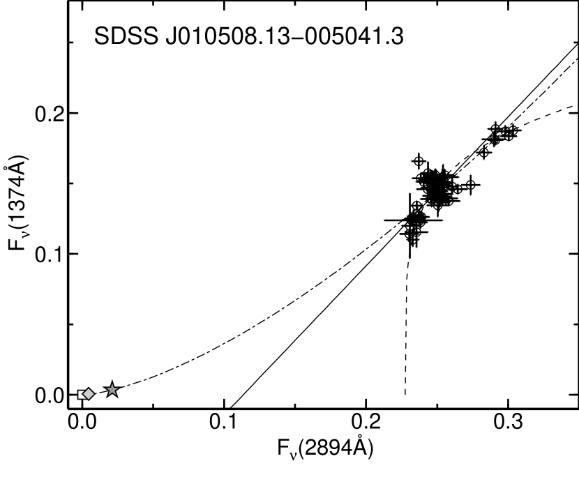
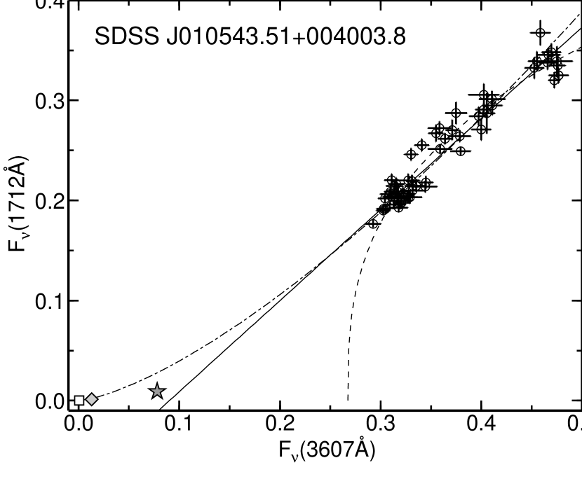
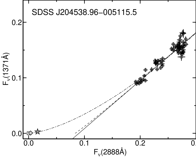
Figure 3: Flux-to-flux diagrams for SDSS J010508.13-005041.3, SDSS J010543.51+004003.8, SDSS J013656.30-004623.7, SDSS J031236.97-011343.1, SDSS J034646.11-004212.8, and SDSS J204538.96-005115.5. The unit of flux is mJy. Open circles with error bars represent the multi-epoch flux data. Square, diamond, and stellate symbols represent the host galaxy flux for the galaxy types E, Sbc, and Im, respectively. Thick, dashed, and dashed-dotted lines represent the best-fit regression of a straight line, a power-law, and a power-law whose power is derived from the wavelength-dependent amplitude of variation of Vanden Berk et al. (2004).

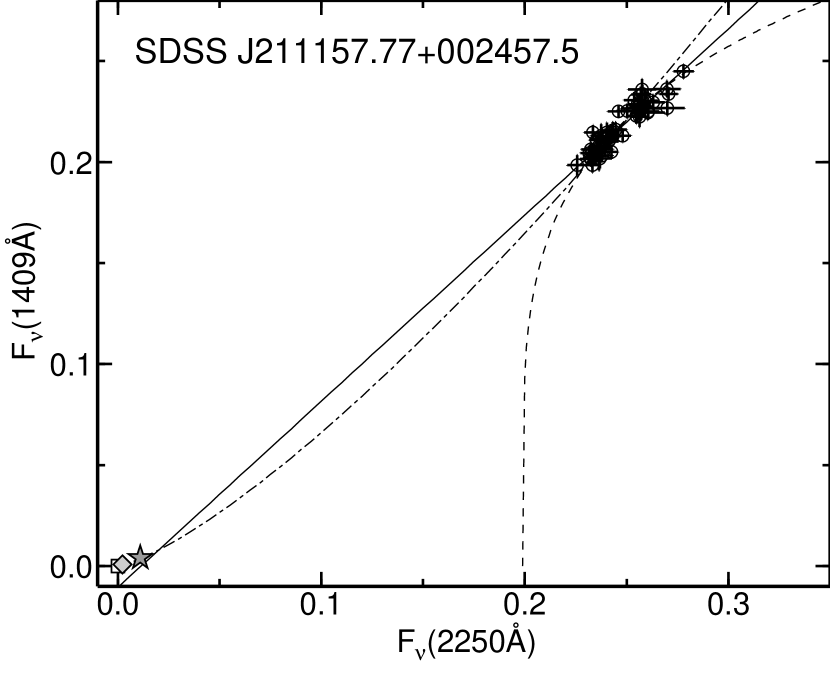
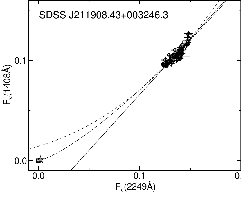
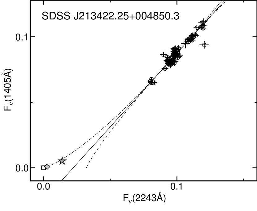
Figure 4: Same as in Figure 3, but for SDSS J211157.77+002457.5, SDSS J211908.43+003246.3, SDSS J212329.46-005052.9, and SDSS J213422.25+004850.3.

In order to examine the color variability of the UV continuum emission of QSOs with flux variation, we applied the flux-to-flux plot analysis as applied to the color variability of optical continuum emission of Seyfert galaxies in Paper I, which was originally proposed by Choloniewski (1981). We plotted the flux data in two different bands observed on the same night in the flux-to-flux diagram, where the flux in longer wavelength is assigned to the $x$-axis and the flux in shorter wavelength is assigned to the $y$-axis. The flux-to-flux plots for all target QSOs are presented in Figures 3 and 4, and the band pair and its effective wavelength in the rest frame for each target are listed in Table 1. The rest wavelength of the shorter-$\lambda$ filter is either $\sim 1400$ Å  or $\sim 1730$ Å , while that of the longer-$\lambda$ is between $2200-3600$ Å.

As shown in Figures 3 and 4, the rest-frame UV flux data in the two different bands are distributed linearly for all targets, and especially for those with large flux variation such a correlation seems very tight. In order to examine the linear relationship between the UV fluxes in the two different bands, both straight-line fitting and power-law fitting to the data in the flux-to-flux diagram were carried out using the fitting code made by Tomita (2005) following the most generalized multivariate least square process given by Jefferys (1980, 1981). The fitting functions adopted for the straight-line fitting and the power-law fitting are $F_{\nu 1}=\alpha\times(F_{\nu_{2}}-F_{\nu_{2}0})$ and $F_{\nu 1}=\alpha\times(F_{\nu_{2}}-F_{\nu_{2}0})^{\beta}$, respectively, because larger contamination of the host galaxy flux is expected in the longer-wavelength flux ($F_{\nu_{2}}$) than in the shorter-wavelength flux ($F_{\nu_{1}}$). The best-fit parameter values and the reduced $\chi^{2}$ values of the straight-line fitting and the power-law fitting are listed in Table 3.

As listed in Table 3, the residuals of the straight-line fitting of the flux-to-flux plots in UV wavelengths are so small that the reduced $\chi^{2}$ is near unity, except for J2045$-$0051. Indeed, according to the $\chi^{2}$-test for the straight-line fitting, the linear relationship is not rejected for 6 of the 10 targets (J0312$-$0113, J0346$-$0042, J2111$+$0024, J2119$+$0032, J2123$-$0050, and J2134$+$0048) at a 1% level of significance. Although the $\chi^{2}$-test rejects the linear relationship at a 1% level of significance for the remaining four targets, no clear curvature can be seen in their flux-to-flux plots. Indeed, no significant improvement of $\chi^{2}$ values applying the power-law fitting instead of the straight-line fitting can be found for two of the four targets (J0136$-$0046 and J2045$-$0051). The larger $\chi^{2}$ values of the straight-line fitting of the four targets are probably caused by another variable component of fluxes that is not synchronized to the UV continuum emission, or by underestimation of the photometric errors. In fact, as will be described in Section 3.3, the reduced $\chi^{2}$ values of the straight-line fitting are significantly decreased for three of the four targets (J0105$-$0050, J0105$+$0040, and J2045$-$0051), and the linear relationship is not rejected at a 1% level of significance for two targets (J0105$-$0050 and J0105$+$0040) when the variable flux component of the SBB is considered. Based on these considerations, we conclude that the UV flux of all of the target QSOs in the two different bands shows a linear correlation during the flux variations.

3.2 Location of Host-Galaxy Component in Flux-to-flux Diagram

The x-intercept of the best-fit linear regression line, $F_{\nu_{2}0}$, is positive for 9 of the 10 targets, as listed in Table 3 (with the exception of J2111$+$0024, for which $F_{\nu_{2}0}$ is consistent to be zero within $2\sigma$ error). Hence, their rest-frame UV colors of the fluxes observed in the two different bands become bluer as they become brighter. However, as presented in the discussion in Paper I, if the sum of the non-variable flux components, such as that of the host galaxy, is located on the fainter extension of the best-fit regression lines of the flux-to-flux plots, the rest-frame UV color is almost constant during the flux variation. In this section, we estimate the host galaxy fluxes of the target QSOs and examine whether the UV colors of the targets show the trend of spectral hardening or remain almost constant during the flux variations.

Since the host galaxies of the target QSOs are not spatially resolved in the SDSS images, we first estimated the stellar mass of the host galaxy from the black hole mass estimated in Section 2.2 and the Magorrian relation (Magorrian et al., 1998), a tight correlation between the central black hole mass and the stellar mass of the bulge of the host galaxy. Next, the host galaxy fluxes in observing bands were converted from the bulge mass using a mass-to-light ratio and an SED of stellar population of the host galaxy. We assumed bulge luminosity as the whole luminosity of the host galaxy because the QSOs at $z\lesssim 2$ are mostly hosted by the bulge-dominated early-type galaxies (e.g., Bahcall et al. 1997; Hutchings et al. 2002; Dunlop et al. 2003; Zakamska et al. 2006)

We used the Magorrian relation presented in Marconi & Hunt (2003),

$$\log M_{\rm BH}=8.28+0.96\times\log(M_{\rm bulge}-10.9),$$ (1)

to estimate the stellar mass of the host galaxy from the black hole mass. The scatter of the correlation was estimated as 0.21 dex by them. Including the scatter of the black hole mass estimation based on the scaling relation for C IV against UV luminosity 0.32 dex presented in Vestergaard & Peterson (2006) we estimated the scatter of the stellar mass of the host galaxy as 0.38 dex, that is, a factor of 2.4 for $1\sigma$ error and 5.8 for $2\sigma$ error. Although the redshift evolution of the Magorrian relation is still uncertain, Peng et al. (2006) suggested that the $M_{\rm BH}/M_{\rm bulge}$ mass ratio increases a factor of $\sim 4$ at $z>1.7$ and Decarli et al. (2010) also showed that it increases a factor of $\sim 7$ at $z=3$ compared to that of the local universe. Therefore, the stellar mass, thus the luminosity of the host galaxy of the targets estimated here, might be systematically overestimated by a factor of $\sim 5$.

Contrary to the morphology, recent studies show that the optical colors of AGN host galaxies at $z\lesssim 1.5$ are slightly bluer than those of quiescent early-type galaxies, indicating a component of newly formed stellar population (e.g., Jahnke, Kuhlbrodt, & Wisotzki 2004b; Sánchez et al. 2004; Nandra et al. 2007; Silverman et al. 2008). In addition, at higher redshift, Jahnke et al. (2004b) showed that the rest-frame UV colors of host galaxies of QSOs at $1.8<z<2.75$ are bluer than that expected from an old stellar population with a formation epoch at $z\sim 5$, suggesting a young stellar population of a few percent of the total mass. Schramm, Wisotzki, & Jahnke (2008) showed that the rest-frame $B-V$ colors of the host galaxies of three QSOs at $z\sim 3$ are close to zero, indicating a substantial contribution from young stars, and a stellar mass-to-light ratio below 1.

Since Kiuchi, Ohta, & Akiyama (2009) demonstrated that most optical SEDs of host galaxies of type-2 AGNs at $0.5<z<1.15$ follow composite SEDs of E to Sbc galaxies of the local universe, and since Barger et al. (2003) showed that the obs-frame $R-HK^{\prime}$ colors of host galaxies of type-2 QSOs at $z=1-2$ are widely scattered between the K-corrected colors of composite SEDs of local E and Im galaxies, we adopt a local Sbc galaxy as a typical model for estimating the mass-to-light ratio and the SED of host galaxies of the target QSOs; we use local E and Im galaxies for the comparison. We use mass-to-light ratios of 20, 2, and 0.5 for E, Sbc, and Im, respectively (Faber & Jackson, 1976; Bell & de Jong, 2001), and calculate the fluxes of the host galaxies in the rest-frame wavelength coverage of the observing filters using an UV-optical spectrum template of nearby galaxies for E, Sbc, and Im presented in Assef et al. (2008).

Figures 3 and 4 present the location of the host galaxy flux of the target QSOs in the flux-to-flux diagrams. The estimated host galaxy fluxes, as described, are listed in Table 4. Figures 3 and 4 clearly show that the location of the host galaxy flux is systematically on the left side of the best-fit regression line. For a typical case of the Sbc-type galaxy, the host galaxy fluxes of 9 of the 10 targets are different from the fainter extension of the best-fit regression line by more than $2\sigma$ error of the host galaxy fluxes, or a factor of 5.8. The only target for which the host galaxy flux is located on the extension of the best-fit regression line within $2\sigma$ error, J2115$+$0024, is in fact $F_{\nu_{2}0}$ consistent to be zero, and the host galaxy flux is estimated to be considerably small. Instead, if we assume the Im-type galaxy for the host galaxy to model recent star-forming activity, as reported for high-redshift QSOs by Schramm et al. (2008), the host-galaxy fluxes of 5 of the 10 targets (J0105$-$0050, J0105$+$0040, J2045$-$0051, J2111$+$0024, and J2134$+$0048) are located on the extension of the best-fit regression line within $2\sigma$ error. However, if the estimated black hole mass using the Magorrian relation at the local universe is systematically smaller by a factor of $\sim 5$ caused by the redshift evolution, the location of the host galaxy flux is on the left side of the best-fit regression line for four of those five targets (except the only target, again J2115$+$0024).

We conclude that most of the target QSOs show spectral hardening in UV wavelengths, that is, the UV continuum emission becomes bluer as it becomes brighter, in spite of maintaining the linear correlations between the QSOs’ two-band flux data. These results suggest that the UV continuum emission of QSOs usually shows spectral hardening, which is consistent with the results reported by Vanden Berk et al. (2004) and Wilhite et al. (2005) from the colors of the differential fluxes or the composite differential spectrum of two-epoch observations for SDSS QSOs.

3.3 Effect of Small Blue Bump

The best-fit parameters and the reduced $\chi^{2}$ values of the straight-line fitting are listed in Table 3. As described in Section 3.1, the reduced $\chi^{2}$ value is so large that the linear relationship is rejected at a 1% level of significance for 4 of the 10 targets (J0105$-$0050, J0105$+$0040, J0136$-$0046, and J2045$-$0051). These larger $\chi^{2}$ values suggest contamination from another variable component of fluxes that is not synchronized to the UV continuum emission.

The SBB consisting of Fe II emission lines and Balmer continuum emission, and the Mg II $\lambda 2798$ emission line, which more or less contaminate our observing bands of the longer-wavelengths, are thought to be the most promising sources for such additional variable components. They are considered to originate in the broad emission-line region (BLR), and moreover, reverberation mapping observations have found the lag of the SBB flux variation behind that of the UV continuum emission for NGC 5548 (Maoz et al., 1993) and the lag of the Mg II emission-line flux variation for NGC 4151 (Metzroth, Onken, & Peterson, 2006). Since the size of the BLR of the target QSOs is estimated to be more than 200 light days for H$\beta$ emission line by the luminosity scaling relation (Kaspi et al., 2005), the flux variation of the SBB emission and the Mg II emission line is not at all synchronized with that of the continuum emission and would provide a scatter around the linear correlation between the fluxes of the UV continuum emission in the two different bands. We estimated the scatter of the linear correlation in the flux-to-flux plots caused by the contaminations from the SBB and Mg II emissions and re-examined the linear relationship of the UV continuum emission in the two different bands.

We first fit the target spectrum obtained from the SDSS database by a power-law model with the spectral windows of $\lambda=1440-1470$Å$\,,1685-1695$Å, $2200-2230$Å, and $4000-4020\AA$, where the spectrum is free from any strong emission lines. The synthesized flux of the spectrum in the photometric band was estimated by convolving the spectrum with the filter transmission curve, and then, the flux of the spectrum was recalibrated by scaling the synthesized flux by the photometric data at the observing date of the spectroscopy that was estimated by interpolating the light curve. The contaminated flux of the SBB and Mg II emissions in the broad-band filter was estimated by subtracting the synthesized flux of the best-fit power-law spectrum from that of the original spectrum. The contaminated fluxes of the SBB and Mg II emissions in the longer wavelength filter are listed in Table 5. Their uncertainties were derived from the error of the power-law fitting.

Next, the $1\sigma$ scatter of the flux variation of the SBB and Mg II emission-line component, $\sigma_{SBB}$, was estimated as $f_{SBB}\times\sigma_{c}/\bar{f_{c}}$, where $f_{SBB}$, $\bar{f_{c}}$, and $\sigma_{c}$ are the contaminated flux of the SBB and Mg II emissions, the average flux, and the $1\sigma$ scatter over the broad-band light curve, respectively. The $\sigma_{SBB}$ is also listed in Table 5.

Finally, assuming that the flux variation of the SBB and Mg II emission line is totally uncorrelated with that of the continuum emission in time, we recalculated the reduced $\chi^{2}$ of the straight-line fitting for the flux-to-flux plots by replacing $\sigma_{obs}$ by $\sqrt{\sigma_{obs}^{2}+\sigma_{SBB}^{2}}$, where $\sigma_{obs}$ is the observational error of the photometry. The new reduced $\chi^{2}$ values of the straight-line fitting in which the scatter caused by the contaminations of the SBB and Mg II emissions is considered, are listed in Table 5.

We found that the reduced $\chi^{2}$ values of the straight-line fitting were significantly decreased for three targets (J0105$-$0050, J0105$+$0040, and J2045$-$0051) out of the four targets, for which the linear relationship was rejected by the $\chi^{2}$ analysis in Section 3.1, and the linear relationship is now not rejected at a 1% level of significance for two targets (J0105$-$0050 and J0105$+$0040). These results strongly indicate that a part of the scatter of the flux-to-flux plot from the best-fit regression line is caused by the contaminations from the SBB and Mg II emission line, and the UV continuum emissions in two different bands of the target QSOs show a tight linear correlation during the flux variations.

4 Discussion

4.1 Comparison with Previous Studies

4.1.1 Vanden Berk et al. (2004)

Vanden Berk et al. (2004) examined the relationship between variability amplitude and the rest-frame wavelength of the UV-optical region from SDSS two-epoch multi-band observations of about 25,000 QSOs, and found a larger amplitude of variation at shorter wavelengths in the UV region of $\lambda<4000$ Å. In this section, the tracks of the flux-to-flux plot of the target QSOs obtained from the photometric monitoring data, which show the hardening trend in the UV region, as presented in the previous sections, are compared with the hardening trend of the amplitude of variation presented in Vanden Berk et al. (2004).

Assuming that the wavelength-dependent amplitude of variation always holds for the flux variation at all times for individual QSOs, a power-law function of $F_{\nu{1}}=\alpha\times F_{\nu{2}}^{\beta}$ in a flux-to-flux plot is obtained, where $\beta=v(\lambda_{1})/v(\lambda_{2})$ is derived from the wavelength-dependent amplitude of variation $v(\lambda)$, presented in Equation 11 of Vanden Berk et al. (2004). Then, we fit the power-law function, $F_{\nu{1}}=\alpha_{2}\times F_{\nu_{2}}^{\beta_{2}}$, to the flux-to-flux plot data of the target QSOs, fixing the parameter $\beta_{2}$ as $\beta_{2}=v(\lambda_{1})/v(\lambda_{2})$, where $\lambda_{1}$ and $\lambda_{2}(\lambda_{1}<\lambda_{2})$ are the effective wavelengths of the observing filters in the rest frame.

Figures 3 and 4 present the fitting of the power-law function to the flux-to-flux plots, and the best-fit parameters and the reduced $\chi^{2}$ values are listed in Table 6. The reduced $\chi^{2}$ value of the power-law fit is comparable to that of the straight-line fit for most of the target QSOs. The slope of the power-law fit seems to be slightly gentler than that of the flux-to-flux plots for J2123$-$0050, and in fact, the reduced $\chi^{2}$ of the power-law fit is slightly larger than that of the straight-line fit even if it is still as small as $\sim 1$. When we refit the power-law function, $F_{\nu{1}}=\alpha_{2}\times F_{\nu_{2}}^{\beta_{2}}$, with both $\alpha_{2}$ and $\beta_{2}$ freed, $\beta_{2}=1.908\pm 0.152$ is derived from the new power-law fit with the reduced $\chi^{2}=0.695$. The $\beta_{2}$ value is slightly different from $v(\lambda_{1})/v(\lambda_{2})$ but would be still consistent with Vanden Berk et al. (2004) within the fitting error and the diversity of QSO properties, and the reduced $\chi^{2}$ becomes comparable to that of the straight-line fit. From these results, we conclude that our results of the hardening trend during the flux variation obtained from the flux-to-flux plots in the rest-frame UV wavelengths are consistent with the hardening trend of the variability amplitude in the UV region presented in Vanden Berk et al. (2004).

4.1.2 Paltani & Walter (1996)

Paltani & Walter (1996) observed the UV spectra of 15 nearby AGNs at different epochs using the IUE satellite. Applying PCA to the multi-epoch spectra and the decomposition to a variable and a non-variable components, they explained the UV variation in almost all their targets as the sum of a variable component of a constant power-law spectral shape and a non-variable component of the SBB, which means that the spectral shape of the UV continuum emission is almost constant during the flux variation. This finding is not consistent with our results that the UV continuum emission becomes bluer as it becomes brighter for most of the target QSOs. In fact, Paltani & Walter (1996) did not estimate the SBB fluxes of the target AGNs by fitting a spectral model of a power-law continuum plux the SBB to their UV spectrum in order to examine the consistency of that method with the conclusion from the decomposition to a variable and a non-variable components. Moreover, as discussed in Section 3.3, the SBB is thought to originate in the BLR and its flux was found to be variable. It is suspected that a sufficient amount of the SBB flux is constant, which explains the constant spectral shape of the UV continuum emission during flux variation.

On the other hand, Paltani & Walter’s finding that one eigenvalue dominated all the others in the PCA of the UV flux variation is consistent with the linear relationship of the fluxes in the two different bands found in the flux-to-flux plots of our target QSOs. The models of the accretion disk predict that the spectral shape of the UV-optical continuum emission depends on the mass accretion rate and the black hole mass; thus, the spectral properties of flux variation would also depend on those AGN properties. Therefore, while it is beyond the scope of this paper, it is very interesting to re-examine the multi-epoch UV spectra of nearby AGNs of Paltani & Walter (1996) using the flux-to-flux plot analysis with accurate estimation of non-variable components such as the host galaxy and also to discuss the luminosity or the black hole mass dependency of the spectral variability of the UV continuum emission.

4.2 Comparison with Accretion Disk Model

We showed that the spectral shape of the optical continuum emission is almost constant during the flux variation for 11 Seyfert galaxies in Paper I, which suggests that the radial temperature profile of an optical emitting region of an accretion disk does not change during the flux variation. On the other hand, we here find that the UV continuum emission becomes bluer as it brightens for most of the target QSOs, while the UV fluxes in the two different bands show a tight linear correlation. This suggests that the temperature structure of the UV emitting region of an accretion disk shows systematic change.

When the mass accretion rate changes in a standard accretion disk model (Shakura & Syunyaev, 1973), the spectral shape of the continuum emission from the accretion disk changes in UV wavelengths while it remains almost constant in optical wavelengths for AGNs whose central black hole mass is larger than $\sim 10^{7-8}M_{\odot}$ (e.g., Kawaguchi, Shimura, & Mineshige 2001). That is because the variation of the mass accretion rate changes the maximum temperature of the accretion disk, which affects the spectral shape of UV continuum emission, while it does not change the radial profile of outer accretion disk of $T(r)\propto r^{-3/4}$ where the optical continuum emission originates, which would result in an almost constant optical continuum spectral shape.

Pereyra et al. (2006) presented that a standard accretion disk model in which the mass accretion rate changed from one epoch to the next could be successfully fitted to the composite differential spectrum of two epochs of observations for hundreds of SDSS QSOs, which is bluer than the composite spectrum of QSOs indicating the spectral hardening of UV continuum emission (Wilhite et al., 2005). However, the composite spectrum represents the average characteristics of QSOs; moreover, the differential spectrum corresponds only to the slope of the linear relationship between fluxes in two different bands in the flux-to-flux plots. Here, we fit a standard accretion disk model with a varying mass accretion rate to the flux-to-flux plots for individual target QSOs, and examine whether the spectral variation of the UV continuum emission during flux variations at various epochs can be described by the standard accretion disk model with various mass accretion rates and a constant black hole mass.

The inner radius of the standard accretion disk model is set as $R_{in}=3Rs$, where $Rs$ is the Schwarzschild radius. The outer radius is set as $R_{out}=1000Rs$, but it is not important for the UV spectrum. A face-on view is assumed to calculate the flux from the accretion disk. Then, a trajectory of the accretion disk model in the flux-to-flux diagram can be traced by changing the mass accretion rate with a constant black hole mass. We fit the trajectory of the accretion disk model to the flux-to-flux plots of the individual target QSOs with a free parameter of black hole mass. Since the observed flux includes the contaminating fluxes of the host galaxy, the SBB and Mg II emission line in addition to the continuum emission, the Sbc-type host galaxy flux estimated in Section 3.2, and the SBB and Mg II contaminating flux estimated in Section 3.3 are added to the trajectory of the accretion disk model before fitting.

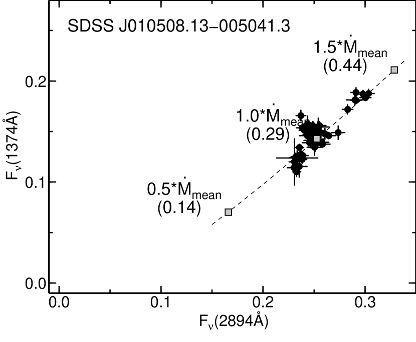
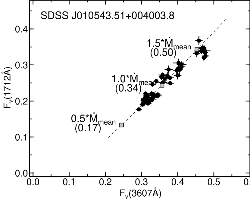
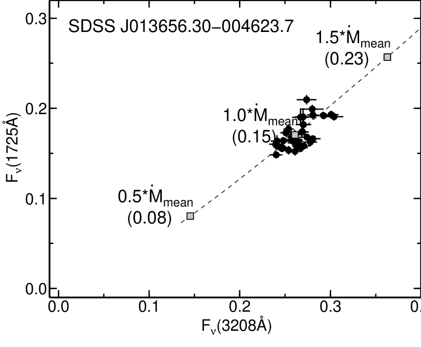
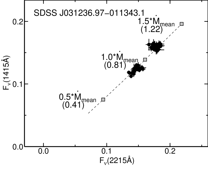
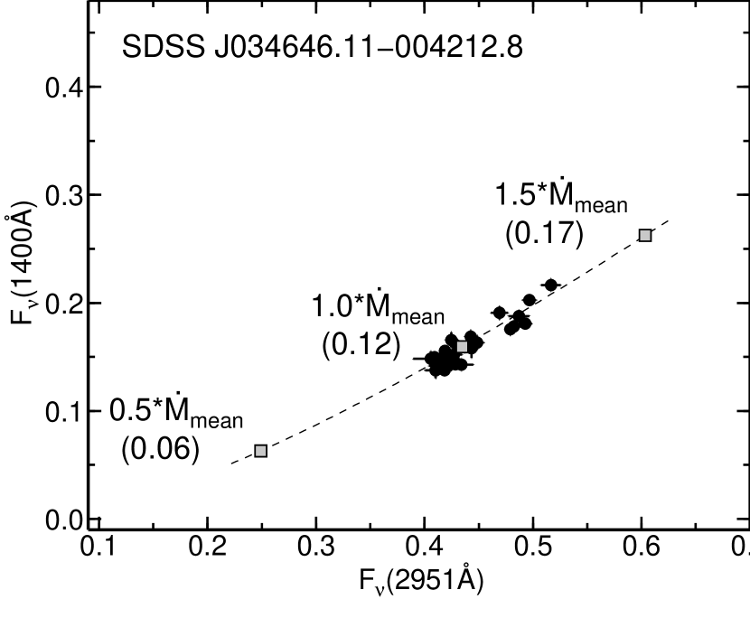
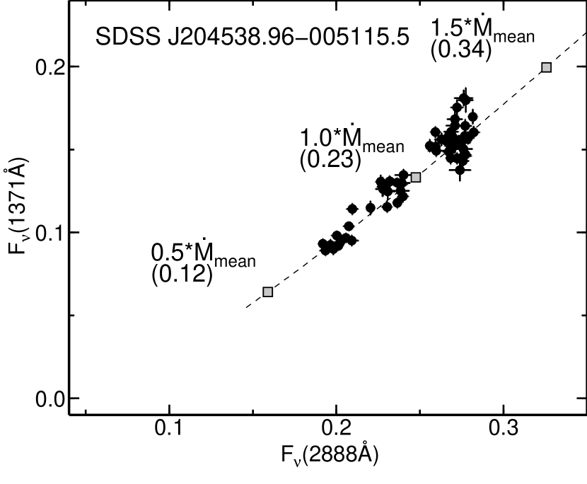
Figure 5: Multi-epoch flux data compared with the standard accretion disk model with varied mass accretion rates and a constant black hole mass for SDSS J010508.13-005041.3, SDSS J010543.51+004003.8, SDSS J013656.30-004623.7, SDSS J031236.97-011343.1, SDSS J034646.11-004212.8, and SDSS J204538.96-005115.5. Open circles with error bars represent the multi-epoch flux data, and a dashed line represents the curve in the flux-to-flux diagram of the best-fit model. Three squares are marked on the best-fit model curve corresponding to 0.5, 1.0, and 1.5 times the mean mass accretion rate that will produce the fluxes averaged over the light curves. The Eddington ratios of the best-fit model are provided in parentheses next to the squares.

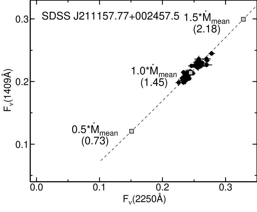
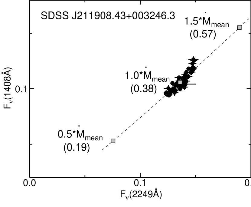
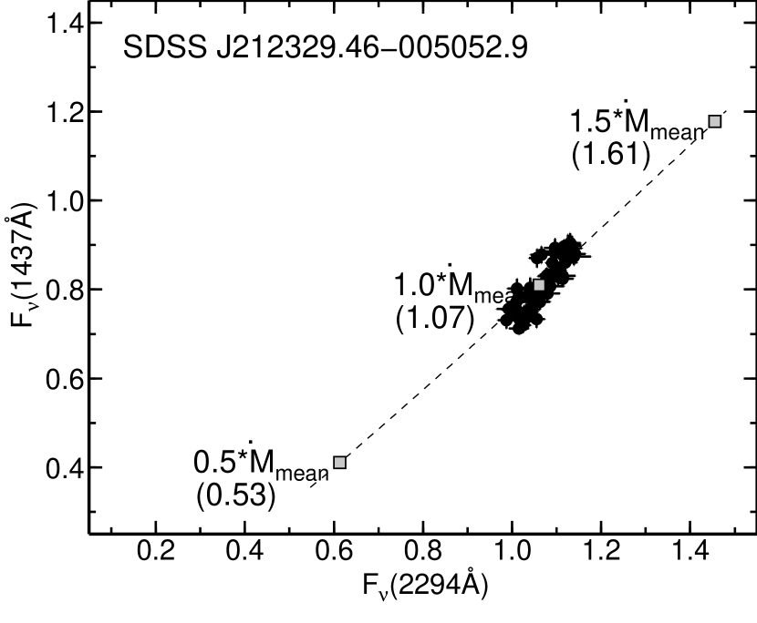
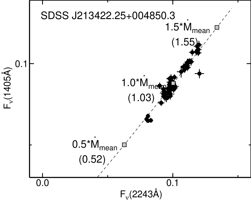
Figure 6: Same as in Figure 5, but for SDSS J211157.77+002457.5, SDSS J211908.43+003246.3, SDSS J212329.46-005052.9, and SDSS J213422.25+004850.3.

Figures 5 and 6 present the best-fit accretion disk model for the flux-to-flux plots of the target QSOs, and the best-fit black hole mass and the reduced $\chi^{2}$ are listed in Table 7. The error of the black hole mass in the table is estimated from the statistical uncertainty of $\chi^{2}$-fitting of the model. As shown in Figures 5 and 6, the flux-to-flux plots can be fitted well by the standard accretion disk model, changing the mass accretion rate with a constant black hole mass. Indeed, the reduced $\chi^{2}$ values of the standard accretion disk model are comparable to those of the straight-line fitting for 9 of the 10 target QSOs, and even for the exception, J2123$-$0050, the reduced $\chi^{2}$ is as small as $\sim 1$. In addition, as shown in Figure 7, the best-fit black hole mass of the standard accretion disk model is consistent with the black hole mass estimated from the emission-line width and the luminosity scaling relation in Section 2.2, within 0.76 dex for $2\sigma$ error of the latter black hole mass estimation. We also calculate the bolometric luminosity of the best-fit standard accretion disk model whose mass accretion rate corresponds to the average flux of the light curve. The ratio of the bolometric luminosity to the specific luminosity in UV, the bolometric correction $L_{\rm bol}/\lambda L_{\lambda}(3000{\rm\AA})$, is listed in Table 7. We find that the bolometric correction is consistent with those obtained for hundreds of type 1 QSOs from Richards et al. (2006), which are distributed between 4 to 9 and whose average value is 5.62. The black hole mass and the luminosity of the best-fit standard accretion disk model fitted to the flux-to-flux plots in UV wavebands are reasonable, and it could be a new technique for estimating a black hole mass of luminous QSOs although the systematic uncertainties should be examined.

As presented in Paper I, the optical color of the best-fit regression line in the flux-to-flux diagram can be regarded as that of the AGN optical continuum, because the optical spectral shape remains almost constant during the flux variation and the colors derived from the flux-to-flux plot analysis of nearby Seyfert galaxies were consistent with those of the standard accretion disk model, $\alpha_{\nu}=1/3$. Although it has long been known that the standard accretion disk model apparently shows a contradiction with observations that the composite spectrum of QSOs is redder than that of the standard accretion disk model (Francis et al., 1991; Vanden Berk et al., 2001), the detailed analyses of the spectral shape of the UV-optical continuum emission of AGNs using flux variation presented here and in Paper I strongly support the standard accretion disk. A possible explanation for the composite spectra being redder is that host galaxy light contaminates the spectra preferentially at longer wavelengths. These results are consistent with the recent analyses of the spectral shape of the optical to near-infrared continuum emission, which comes from the accretion disk by flux variations (Tomita et al., 2006) and polarizations (Kishimoto et al., 2008).

However, it has a critical difficulty of considering the variation of global accretion rate of a standard accretion disk as a primary source of flux variation of QSOs. The timescale of changes of the global mass accretion rate is believed to correspond to the viscous timescale (e.g., Pringle 1981; Frank et al. 2002), which is about $\sim 10^{6}$ years for our target QSOs and much longer than the timescale of the flux variation we observed. Clearly, further study of the flux variation mechanism is desired, which can explain the observed properties of spectral variations of the UV-optical continuum emission of AGNs, suggesting a variation of the characteristic temperature of an accretion disk.

5 Summary

We examined the spectral variability of UV continuum emission of AGNs based on the multi-epoch photometric data of 10 SDSS QSOs in the Stripe 82. The target redshift was $z=1.05,1.54,1.71,2.35\pm 0.05$ in which strong broad lines such as Ly$\alpha$ and C IV do not contaminate SDSS filters. The target luminosity was about $\lambda L_{\lambda}(3000{\rm\AA})\sim 10^{46-47}$ erg s^-1, the black hole mass was estimated to be about $10^{9-10}M_{\odot}$ based on the luminosity scaling relations for C IV or Mg II emission lines and their line width, and the mean Eddington ratio was between $0.1-1.2$. All target QSOs showed significant flux variation within 7 years of observation, or $2-3.5$ years in the rest-frame.

We plotted the flux data in two different bands (shorter-$\lambda_{rest}\sim 1400$ Å  or $\sim 1730$ Å, longer-$\lambda_{rest}\sim 2200$ Å$-3600$ Å) observed on the same night in the flux-to-flux diagram and found a strong linear correlation between the fluxes in the two different bands during the flux variations for all target QSOs. The linear relationship was not rejected for 6 of the 10 targets at a 1$\%$ level of significance based on the $\chi^{2}$-test for straight-line fitting. Even for the remaining four targets, no clear curvature could be seen in their flux-to-flux plots; no significant improvement of $\chi^{2}$ values by the power-law fitting than those of the straight-line fitting could be found for two of the four targets, and the reduced $\chi^{2}$ values of the straight-line fitting were significantly decreased for three of the four targets when the contamination of the SBB was considered.

We then examined the location of the host galaxy flux in the flux-to-flux diagram. The stellar mass of the host galaxy was estimated from the black hole mass on the basis of the Magorrian relation (Marconi & Hunt, 2003); then, the host galaxy flux was estimated from the stellar mass using the mass-to-light ratio and the SED of a local Sbc galaxy (Bell & de Jong, 2001; Assef et al., 2008). We found that the location of the host galaxy flux was systematically on the left side of the best-fit regression line for 9 of the 10 targets; that is, the UV continuum emission becomes bluer as it brightens for most of the target QSOs in spite of holding their linear correlations between the two-band flux data. This trend of spectral hardening in UV wavelengths is consistent with the findings of Vanden Berk et al. (2004). Indeed, we found that the flux-to-flux plots of the target QSOs could be fitted well by a power-law function assuming the wavelength-dependent variability amplitude of QSOs.

We presented in Paper I that the spectral shape of the optical continuum emission of AGNs remains almost constant and that its color is consistent with that of the standard accretion disk model, $\alpha_{\nu}=1/3$. Then, in the present paper, we fit a standard accretion disk model with a changing mass accretion rate and a constant black hole mass to the UV flux-to-flux plots for the individual target QSOs, and found that the spectral variation of the UV continuum emission during flux variations at various epochs could be described by the standard accretion disk model with varied mass accretion rates. The black hole mass and the bolometric luminosity from the best-fit standard accretion disk model were reasonable. Although it has long been known that the composite spectrum of QSOs is redder than that of the standard accretion disk model, the detailed analyses of the spectral shape of the UV-optical continuum emission of AGNs using flux variation strongly support the standard accretion disk model. However, the variation timescale of the global mass accretion rate was considered to be too large to explain the flux variations within a few years, and further study of the flux variation mechanism is desired.

Figure 1: Light curves in the two SDSS filters (Table 1) for SDSS J010508.13-005041.3, SDSS J010543.51+004003.8, SDSS J013656.30-004623.7, SDSS J031236.97-011343.1, SDSS J034646.11-004212.8, and SDSS J204538.96-005115.5. The wavelengths provided in the figures are the rest-frame effective wavelengths of the two filters.

Figure 2: Same as in Figure 1, but for SDSS J211157.77+002457.5, SDSS J211908.43+003246.3, SDSS J212329.46-005052.9, and SDSS J213422.25+004850.3.

Figure 7: The ratio of the black hole mass estimated from the luminosity scaling relation and the emission-line width to that of the best-fit standard accretion disk model applied to the flux-to-flux plots.

Table 1: Light Curve of Target QSOs

Object	Redshift	Filter1	Filter2	Rest $\lambda_{1}$[Å]	Rest $\lambda_{2}$[Å]	Number of Data	$\bar{F}_{\nu 1}$	$\sigma_{\nu 1}$	$\bar{F}_{\nu 2}$	$\sigma_{\nu 2}$
SDSS J010508.13$-$005041.3	1.585	u	i	1374	2894	68	0.146	0.017	0.251	0.017
SDSS J010543.51$+$004003.8	1.074	u	i	1712	3607	57	0.238	0.056	0.361	0.059
SDSS J013656.30$-$004623.7	1.716	g	z	1725	3288	39	0.169	0.015	0.263	0.015
SDSS J031236.97$-$011343.1	2.311	g	i	1415	2215	67	0.140	0.019	0.161	0.016
SDSS J034646.11$-$004212.8	1.535	u	i	1400	2951	33	0.156	0.020	0.436	0.030
SDSS J204538.96$-$005115.5	1.590	u	i	1371	2888	57	0.133	0.026	0.246	0.029
SDSS J211157.77$+$002457.5	2.325	g	i	1409	2250	52	0.216	0.012	0.245	0.012
SDSS J211908.43$+$003246.3	2.327	g	i	1408	2249	52	0.106	0.008	0.136	0.007
SDSS J212329.46$-$005052.9	2.261	g	i	1437	2294	62	0.808	0.058	1.064	0.043
SDSS J213422.25$+$004850.3	2.336	g	i	1405	2243	64	0.087	0.011	0.100	0.010

Table 2: Characteristics of Target QSOs

Object	Radio	$\log(\lambda L_{\lambda}(1350\AA)$	$\log(\lambda L_{\lambda}(3000\AA)$	$\sigma($C IV$)$	$\sigma($Mg II$)$	$\log(M_{BH}($C IV$))$	$\log(M_{BH}($Mg II$))$	$L_{bol}/L_{Edd}$
		[ergs s-1]	[ergs s-1]	[km s-1]	[km s-1]	[$M_{\odot}]$	[$M_{\odot}]$
J0105$-$0050	$\times$	46.30	46.16	2027	1720	9.29	9.21	0.33
J0105$+$0040	$\times$	—	45.94	—	1848	—	9.19	0.27
J0136$-$0046	$\times$	46.31	46.26	*4465	1340	*9.93	8.99	0.74
J0312$-$0113	$\times$	46.47	46.40	1498	—	9.10	—	0.94
J0346$-$0042	not covered	46.32	46.35	*1358	1746	*8.92	9.31	0.49
J2045$-$0051	not covered	46.26	46.16	2066	1622	9.20	9.09	0.34
J2111$+$0024	$\times$	46.70	46.56	2392	—	9.64	—	0.37
J2119$+$0032	$\times$	46.37	46.34	1323	—	8.94	—	1.13
J2123$-$0050	$\times$	47.24	47.20	2541	—	9.99	—	0.78
J2134$+$0048	$\times$	46.24	46.17	*3731	—	*9.74	—	0.12

Table 3: Straight-line and Power-law Fits to Flux-to-flux Plots

Object	Straight-line Fit				Power-law Fit
	$\alpha$	F${}_{\nu 2}0$	Reduced $\chi^{2}$		$\alpha$	F${}_{\nu 2}0$	$\beta$	Reduced $\chi^{2}$
J0105$-$0050	1.057 $\pm$ 0.060	0.113 $\pm$ 0.008	1.70		0.310 $\pm$   0.023	0.228 $\pm$ 0.004	0.194 $\pm$   0.029	1.23
J0105$+$0040	0.910 $\pm$ 0.025	0.090 $\pm$ 0.007	1.86		0.589 $\pm$   0.037	0.267 $\pm$ 0.012	0.350 $\pm$   0.049	1.47
J0136$-$0046	1.082 $\pm$ 0.132	0.107 $\pm$ 0.019	1.81		1.683 $\pm$   3.412	$-$0.145 $\pm$ 2.779	2.569 $\pm$ 17.297	1.84
J0312$-$0113	1.155 $\pm$ 0.047	0.040 $\pm$ 0.005	0.74		0.466 $\pm$ 22.985	$-$0.680 $\pm$ 7.208	6.960 $\pm$ 59.681	0.72
J0346$-$0042	0.647 $\pm$ 0.039	0.193 $\pm$ 0.015	1.26		0.657 $\pm$   0.660	$-$0.016 $\pm$ 1.050	1.810 $\pm$   4.048	1.29
J2045$-$0051	0.865 $\pm$ 0.022	0.090 $\pm$ 0.004	2.71		0.903 $\pm$   0.307	0.083 $\pm$ 0.055	1.048 $\pm$   0.385	2.76
J2111$+$0024	0.992 $\pm$ 0.074	0.028 $\pm$ 0.016	0.57		0.427 $\pm$   0.121	0.199 $\pm$ 0.030	0.221 $\pm$   0.141	0.53
J2119$+$0032	1.112 $\pm$ 0.069	0.041 $\pm$ 0.006	0.83		4.180 $\pm$ 16.912	$-$0.127 $\pm$ 1.163	2.754 $\pm$ 12.147	0.80
J2123$-$0050	1.453 $\pm$ 0.116	0.507 $\pm$ 0.045	0.69		1.565 $\pm$   0.167	0.731 $\pm$ 0.559	0.598 $\pm$   1.005	0.70
J2134$+$0048	1.131 $\pm$ 0.039	0.023 $\pm$ 0.003	0.97		0.905 $\pm$   0.435	0.032 $\pm$ 0.021	0.868 $\pm$   0.279	0.99

Table 4: Estimation of Host Galaxy Flux

Object	$F_{\nu 1}$(E)	$F_{\nu 2}$(E)	$F_{\nu 1}$(Sbc)	$F_{\nu 2}$(Sbc)	$F_{\nu 1}$(Im)	$F_{\nu 2}$(Im)
J0105$-$0050	6.7E$-$07	4.1E$-$05	6.4E$-$04	4.4E$-$03	3.5E$-$03	2.1E$-$02
J0105$+$0040	1.8E$-$06	7.0E$-$04	1.4E$-$03	1.3E$-$02	9.0E$-$03	7.8E$-$02
J0136$-$0046	4.6E$-$07	9.3E$-$05	3.5E$-$04	2.4E$-$03	2.3E$-$03	1.2E$-$02
J0312$-$0113	2.3E$-$07	1.0E$-$06	2.2E$-$04	6.0E$-$04	1.2E$-$03	3.0E$-$03
J0346$-$0042	7.5E$-$07	6.5E$-$05	7.2E$-$04	5.0E$-$03	3.9E$-$03	2.4E$-$02
J2045$-$0051	5.4E$-$07	3.3E$-$05	5.1E$-$04	3.4E$-$03	2.8E$-$03	1.6E$-$02
J2111$+$0024	7.9E$-$07	3.7E$-$06	7.6E$-$04	2.2E$-$03	4.2E$-$03	1.1E$-$02
J2119$+$0032	1.5E$-$07	6.8E$-$07	1.4E$-$04	4.0E$-$04	7.6E$-$04	2.0E$-$03
J2123$-$0050	2.0E$-$06	9.2E$-$06	1.9E$-$03	5.4E$-$03	1.1E$-$02	2.7E$-$02
J2134$+$0048	9.9E$-$07	4.7E$-$06	9.5E$-$04	2.7E$-$03	5.2E$-$03	1.4E$-$02

Note. — Flux in units of mJy.

Table 5: Small Blue Bump Flux

Object	$F_{\nu 2}$(SBB)	$\sigma_{\nu 2}$(SBB)	reduced $\chi^{2}$
			$\sigma_{\nu 2}$(SBB) included	not included
J0105$-$0050	4.78E$-$02 $\pm$ 3.15E$-$03	3.19E$-$03	1.41	1.70
J0105$+$0040	6.46E$-$02 $\pm$ 3.82E$-$03	1.04E$-$02	0.98	1.86
J0136$-$0046	1.24E$-$02 $\pm$ 2.87E$-$03	7.07E$-$04	1.80	1.81
J0312$-$0113	3.15E$-$03 $\pm$ 1.17E$-$03	3.10E$-$04	0.73	0.74
J0346$-$0042	3.58E$-$02 $\pm$ 7.85E$-$03	2.50E$-$03	1.17	1.26
J2045$-$0051	3.88E$-$02 $\pm$ 3.73E$-$03	4.50E$-$03	1.69	2.71
J2111$+$0024	1.33E$-$02 $\pm$ 1.88E$-$03	6.68E$-$04	0.56	0.57
J2119$+$0032	6.50E$-$05 $\pm$ 1.45E$-$03	3.56E$-$06	0.83	0.83
J2123$-$0050	5.55E$-$02 $\pm$ 7.60E$-$03	2.26E$-$03	0.69	0.69
J2134$+$0048	5.05E$-$03 $\pm$ 7.64E$-$04	4.88E$-$04	0.96	0.97

Note. — Flux in units of mJy.

Table 6: Vanden Berk Model Fits to Flux-to-flux Plots

Object	$\alpha_{2}$	$\beta_{2}$	Reduced $\chi^{2}$
			Vanden Berk et al. (2004)	Straight-line
J0105$-$0050	1.164 $\pm$ 0.007	1.505	1.89	1.70
J0105$+$0040	1.040 $\pm$ 0.006	1.419	2.11	1.86
J0136$-$0046	1.056 $\pm$ 0.008	1.375	1.82	1.81
J0312$-$0113	1.539 $\pm$ 0.008	1.315	0.72	0.74
J0346$-$0042	0.544 $\pm$ 0.004	1.499	1.43	1.26
J2045$-$0051	1.107 $\pm$ 0.005	1.506	2.82	2.71
J2111$+$0024	1.369 $\pm$ 0.006	1.315	0.62	0.57
J2119$+$0032	1.460 $\pm$ 0.007	1.315	0.83	0.83
J2123$-$0050	0.745 $\pm$ 0.003	1.314	1.07	0.69
J2134$+$0048	1.805 $\pm$ 0.008	1.316	0.98	0.97

Table 7: Standard Accretion Disk Model Fit to Flux-to-flux Plots

Object	$\log(M_{BH}/M_{\odot})$	Reduced $\chi^{2}$		Bolometric Correction
		AD model	Straight-line
J0105$-$0050	9.38${}^{+0.01}_{-0.01}$	1.86	1.70	6.04
J0105$+$0040	9.18${}^{+0.02}_{-0.01}$	2.03	1.86	7.00
J0136$-$0046	9.70${}^{+0.01}_{-0.01}$	1.92	1.81	5.50
J0312$-$0113	9.26${}^{+0.01}_{-0.01}$	0.72	0.74	7.30
J0346$-$0042	9.90${}^{+0.01}_{-0.01}$	1.25	1.26	4.80
J2045$-$0051	9.46${}^{+0.01}_{-0.01}$	2.71	2.71	5.73
J2111$+$0024	9.24${}^{+0.02}_{-0.02}$	0.55	0.57	8.63
J2119$+$0032	9.43${}^{+0.01}_{-0.01}$	0.93	0.83	5.95
J2123$-$0050	9.84${}^{+0.01}_{-0.01}$	1.11	0.69	5.84
J2134$+$0048	9.02${}^{+0.02}_{-0.02}$	1.06	0.97	8.88

References

- Assef et al. (2008) Assef, R. J., et al. 2008, ApJ, 676, 286
- Bahcall et al. (1997) Bahcall, J. N., Kirhakos, S., Saxe, D. H., & Schneider, D. P. 1997, ApJ, 479, 642
- Barger et al. (2003) Barger, A. J., Cowie, L. L., Capak, P., Alexander, D. M., Bauer, F. E., Fernandez, E., Brandt, W. N., Garmire, G. P., & Hornschemeier, A. E. 2003, AJ, 126, 632
- Becker et al. (1995) Becker, R. H., White, R. L., & Helfand, D. J. 1995, ApJ, 450, 559
- Bell & de Jong (2001) Bell, E. F., & de Jong, R. S. 2001, ApJ, 550, 212
- Choloniewski (1981) Choloniewski, J. 1981, Acta Astronomica, 31, 293
- Collier et al. (1999) Collier, S., Horne, K., Wanders, I., & Peterson, B. M. 1999, MNRAS, 302, L24
- Courvoisier et al. (1996) Courvoisier, T. J.-L., Paltani, S., & Walter, R. 1996, A&A, 308, L17
- Decarli et al. (2010) Decarli, R., Falomo, R., Treves, A., Labita, M., Kotilainen, J. K., & Scarpa, R. 2010, MNRAS, 402, 2453
- Dunlop et al. (2003) Dunlop, J. S., McLure, R. J., Kukula, M. J., Baum, S. A., O’Dea, C. P., & Hughes, D. H. 2003, MNRAS, 340, 1095
- Faber & Jackson (1976) Faber, S. M., & Jackson, R. E. 1976, ApJ, 204, 668
- Francis et al. (1991) Francis, P. J., Hewett, P. C., Foltz, C. B., Chaffee, F. H., Weymann, R. J., & Morris, S. L. 1991, ApJ, 373, 465
- Frank et al. (2002) Frank, J., King, A., & Raine, D. J. 2002, Accretion Power in Astrophysics, by Juhan Frank and Andrew King and Derek Raine, pp. 398. ISBN 0521620538. Cambridge, UK: Cambridge University Press, February 2002.,
- Giveon et al. (1999) Giveon, U., Maoz, D., Kaspi, S., Netzer, H., & Smith, P. S. 1999, MNRAS, 306, 637
- Hawkins (1993) Hawkins, M. R. S. 1993, Nature, 366, 242
- Hutchings et al. (2002) Hutchings, J. B., Frenette, D., Hanisch, R., Mo, J., Dumont, P. J., Redding, D. C., & Neff, S. G. 2002, AJ, 123, 2936
- Jahnke et al. (2004a) Jahnke et al. 2004, ApJ, 614, 568
- Jahnke et al. (2004b) Jahnke, K., Kuhlbrodt, B., & Wisotzki, L. 2004, MNRAS, 352, 399
- Jefferys (1980) Jefferys, W. H. 1980, AJ, 85, 177
- Jefferys (1981) Jefferys, W. H. 1981, AJ, 86, 149
- Kaspi et al. (2005) Kaspi, S., Maoz, D., Netzer, H., Peterson, B. M., Vestergaard, M., & Jannuzi, B. T. 2005, ApJ, 629, 61
- Kawaguchi et al. (1998) Kawaguchi, T., Mineshige, S., Umemura, M., & Turner, E. L. 1998, ApJ, 504, 671
- Kawaguchi et al. (2001) Kawaguchi, T., Shimura, T., & Mineshige, S. 2001, ApJ, 546, 966
- Kishimoto et al. (2008) Kishimoto, M., Antonucci, R., Blaes, O., Lawrence, A., Boisson, C., Albrecht, M., & Leipski, C. 2008, Nature, 454, 492
- Kiuchi et al. (2009) Kiuchi, G., Ohta, K., & Akiyama, M. 2009, ApJ, 696, 1051
- Krolik et al. (1991) Krolik, J. H., Horne, K., Kallman, T. R., Malkan, M. A., Edelson, R. A., & Kriss, G. A. 1991, ApJ, 371, 541
- Magorrian et al. (1998) Magorrian, J., et al. 1998, AJ, 115, 2285
- Maoz et al. (1993) Maoz, D., et al. 1993, ApJ, 404, 576
- Marconi & Hunt (2003) Marconi, A., & Hunt, L. K. 2003, ApJ, 589, L21
- Metzroth, Onken, & Peterson (2006) Metzroth, K. G., Onken, C. A., & Peterson, B. M. 2006, ApJ, 647, 901
- Nandra et al. (2007) Nandra, K., Georgakakis, A., Willmer, C. N. A., Cooper, M. C., Croton, D. J., Davis, M., Faber, S. M., Koo, D. C., Laird, E. S., & Newman, J. A. 2007 AJ, 660, L11
- Paltani & Walter (1996) Paltani, S., & Walter, R. 1996, A&A, 312, 55
- Peng et al. (2006) Peng, C. Y., Impey, C. D., Rix, H.-W., Kochanek, C. S., Keeton, C. R. Falco, E. E., Leher, J., & McLeod, B. A. 2006, ApJ, 649, 616
- Pereyra et al. (2006) Pereyra, N. A., Vanden Berk, D. E., Turnshek, D. A., Hillier, D. J., Wilhite, B. C., Kron, R. G., Schneider, D. P., & Brinkmann, J. 2006, ApJ, 642, 87
- Pringle (1981) Pringle, J. E. 1981, ARA&A, 19, 137
- Rees (1984) Rees, M. J. 1984, ARA&A, 22, 471
- Richards et al. (2006) Richards, G. T., et al. 2006, ApJS, 166, 470
- Richards et al. (2009) Richards, G. T., et al. 2009, ApJS, 180, 67
- Rodriguez-Pascual et al. (1997) Rodriguez-Pascual, P. M., et al. 1997, ApJS, 110, 9
- Sakata et al. (2010) Sakata, Y., Minezaki, T., Yoshii, Y., Kobayashi, Y., Koshida, S., Aoki, T., Enya, K., Tomita, H., Suganuma, M., Katsuno U. Y., & Sugawara, S. 2010, ApJ, 711, 461 (Paper I)
- Sánchez et al. (2004) Sánchez et al. 2004, ApJ, 614, 586
- Santos-Lleo et al. (1995) Santos-Lleo, M., Clavel, J., Barr, P., Glass, I. S., Pelat, D., Peterson, B. M., & Reichert, G. 1995, MNRAS, 274, 1
- Schramm et al. (2008) Schramm, M., Wisotzki, L., & Jahnke, K. 2008, A&A, 478, 311
- Shakura & Syunyaev (1973) Shakura, N. I., & Syunyaev, R. A. 1973, A&A, 24, 337
- Silverman et al. (2008) Silverman, J. D. et al. 2008 ApJ, 675, 1025
- Tomita (2005) Tomita, H. 2005, PhD thesis, Department of Astronomy, Graduate School of Science, Univ. of Tokyo
- Tomita et al. (2006) Tomita, H., Yoshii, Y., Kobayashi, Y., Minezaki, T., Enya, K., Suganuma, M., Aoki, T., Koshida, S., & Yamauchi, M. 2006, ApJ, 652, L13
- Torricelli-Ciamponi et al. (2000) Torricelli-Ciamponi, G., Foellmi, C., Courvoisier, T. J.-L., & Paltani, S. 2000, A&A, 358, 57
- Trump et al. (2009) Trump, J. R., et al. 2009, ApJ, 700, 49
- Vanden Berk et al. (2001) Vanden Berk, D. E., et al. 2001, AJ, 122, 549
- Vanden Berk et al. (2004) Vanden Berk, D. E., et al. 2004, ApJ, 601, 692
- Vestergaard & Peterson (2006) Vestergaard, M., & Peterson, B. M. 2006, ApJ, 641, 689
- Wamsteker et al. (1990) Wamsteker, W., et al. 1990, ApJ, 354, 446
- Webb & Malkan (2000) Webb, W., & Malkan, M. 2000, ApJ, 540, 652
- Wilhite et al. (2005) Wilhite, B. C., Vanden Berk, D. E., Kron, R. G., Schneider, D. P., Pereyra, N., Brunner, R. J., Richards, G. T., & Brinkmann, J. V. 2005, ApJ, 633, 638
- Wilhite et al. (2008) Wilhite, B. C., Brunner, R. J., Grier, C. J., Schneider, D. P., & vanden Berk, D. E. 2008, MNRAS, 383, 1232
- Wold et al. (2007) Wold, M., Brotherton, M. S., & Shang, Z. 2007, MNRAS, 375, 989
- Xu et al. (2008) Xu, Y., Bian, W.-H., Yuan, Q.-R., & Huang, K.-L. 2008, MNRAS, 389, 1703
- Zakamska et al. (2007) Zakamska, N. L., Strauss, M. A., Krolik, J. H., Ridgway, S. E. Schmidt, G. D., Smith, P. S., Heckman, T. M.; Schneider, D. P., Hao, L., & Brinkmann, J. AJ, 132, 1496