Gluon production on two centers and the effective action approach.

Abstract

Application of the effective action formalism is studied for processes in which the reggeons may split. It is shown that the gluon production on two centers is described by the contribution of the Reggeon-to-two-Reggeons-plus-Particle vertex supplemented by certain singular contributions from the double gluon exchange. The rules for longitudinal integrations are established from the comparison to perturbative QCD amplitude. Convenient expressions for application to the inclusive gluon production are derived.

1 Introduction

In the framework of the perturbative QCD, in the Regge kinematics, particle interaction can be described by the exchange of reggeized gluons which emit and absorb real gluons and also may split into several reggeized gluons. Emission of real gluons from reggeized gluons is described by effective vertices introduced in  [1] and  [2] for non-split and split reggeons. Originally both type of vertices were calculated directly from the relevant simple Feynman diagrams in the Regge kinematics. Later a powerful effective action formalism was proposed in  [3], which considers reggeized and normal gluons as independent entities from the start and thus allows to calculate all QCD diagrams in the Regge kinematics automatically and in a systematic and self-consistent way. However the resulting expressions are 4-dimensional and need reduction to the final 2-dimensional transverse form. This reduction is trivial for tree diagrams but becomes less trivial for diagrams with loops.

In the paper of two co-authors of the present paper (M.A.B. and M.I.V.)  [4] it was demonstrated that the diffractive amplitude for the production of a real gluon calculated by means of the effective action and based on the transition of a Reggeon into one or two Reggeons and Particle (R$\to$R(R)P transition), after integration over longitudinal variables, coincides with the results calculated in terms of the above-mentioned effective vertices (in the purely tranverse ”BFKL-Bartels formalism”). However in the process of reduction to the transverse form a certain prescription had to be used to give sense to divergent integrals.

In this paper we study a more general case: the gluon production off two different targets. In this case, in the lowest order, with which we restrict ourselves, the production amplitude by itself is a tree diagram, without any internal integrations. Longitudinal integrals appear only in the inclusive cross-section. Our purpose is twofold. First we analyze application of the effective action formalism to the processes where the number of reggeons can be changed (from one to two in our case). As we shall show this application requires a careful study of kinematical regions in which particular diagrams generated by the effective action or even parts of these diagrams are to be taken into account. A separate problem is understanding in which sence singularities which appear in these diagrams when the ”-” components of the momenta transferred to the two targets (”energies”), $q_{1,2-}$, vanish are to be understood. Comparison with the standard perturbation approach allows to solve this problem. Note that this latter point was studied in  [5, 6] for simpler diagrams, without reggeon proliferation.

Our second aim is to obtain convenient expressions for the production amplitudes which can be used for the calculation of the inclusive cross-sections. The essential region for the integration over transferred energies involved in this calculation is $q_{1,2-}>>p_{-}$, where $p_{-}$ is the energy of the emitted gluon. The amplitude can be drastically simplfied in this region and transformed to the expression convenient for the following integrations.

Our results show that in the general kinematics the production amplitude is almost completely given by the contribution from the R$\to$RRP effective vertex derived in  [4]. The pole at $q_{1,2-}=0$ should be taken in the principal values prescription, in agreement with the assumption made in  [4]. However the contribution from the R$\to$RRP vertex should be supplemented by terms proportional to $\delta(q_{1,2-})$ coming from the double reggeon exchange.

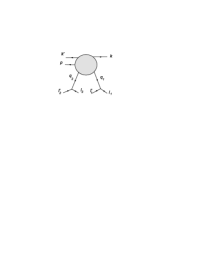
Figure 1: Production amplitude off two scattering centers

2 Kinematics and the target lines

We study the production amplitude on two centers shown in Fig. 1 in the Regge kinematics. For simplicity we consider the quark as the projectile and scalar quarks as the two scattering centers. We consider the central region so that both $(kp)$ and $(lp)$ are large. This means that $k_{+}p_{-}$ and $l_{-}p_{+}$ are much greater than the typical transverse momentum squared $p_{\perp}^{2}$. If $p_{+}=xk_{+}$ then our region of $x$ is

$$\frac{|p_{\perp}^{2}|}{s}<<x<<1.$$ (1)

Our longitudinal conservation laws are

$$p_{+}+k^{\prime}_{+}=k_{+},\ \ p_{-}+q_{1-}+q_{2_{-}}=0,$$ (2)

where we neglected $q_{1+}$, $q_{2+}$ and $k^{\prime}_{-}$.

We consider both targets at the same initial momentum $l_{1}=l_{2}=l$ in the center of mass system with $l_{+}=l_{\perp}=0$. The transferred momenta in the two collisions are $q_{1}$ and $q_{2}$. The mass-shell conditions give

$$2q_{1}l+q_{1}^{2}=2q_{2}l+q_{2}^{2}=0.$$ (3)

The initial projectile momentum $k$ has $k_{-}=k_{\perp}=0$. Our Regge kinematics requires that $q_{1-},q_{2-}<<l_{-}$. So we put $q_{1-}=\xi_{1}l_{-}$ and $q_{2-}=\xi_{2}l_{-}$ with $\xi_{1,2}<<1$. The parameters $\xi_{1}$ and $\xi_{2}$ are actually the conventional Sudakov variables for the transverred momenta $q_{1}$ and $q_{2}$. From

$$q_{1+}=l_{1+}=-\frac{{l^{\prime}_{1\perp}}^{2}}{2l^{\prime}_{1-}}$$

it follows that

$$q_{1}^{2}=2q_{1+}q_{1-}+q_{1\perp}^{2}=(1-\xi_{1})q_{1\perp}^{2}\simeq q_{1\perp}^{2},$$

so that $q_{1}$ is almost a purely transverse momentum. as well as $q_{2}$.

In practical applications we use the axial gauge in which the gluon field $V$ satisfies $(Vl)=0$ and its propagator is

$$P_{\mu\nu}(q)=\frac{h_{\mu\nu}(q)}{q^{2}},\ \ h_{\mu\nu}(q)=g_{\mu\nu}-\frac{l_{\mu}q_{\nu}+q_{\mu}l_{\nu}}{(ql)}.$$ (4)

Coupling to the scalar targets generates vectors

$$P_{\mu}(q)=P_{\mu\nu}(2l^{\nu}+q^{\nu})=P_{\mu\nu}q^{\nu}=-l_{\mu}\frac{q^{2}}{(ql)}\,\frac{1}{q^{2}}=2l_{\mu}\frac{1}{q_{\perp}^{2}},$$ (5)

where $q=q_{1}$ or $q=q_{2}$. So in fact we can study the amplitude with amplutated target lines and external legs $P_{\mu_{1}}(q_{1})$ and $P_{\mu_{2}}(q_{2})$.

3 Gluon emission in the effective action formalism

In the effective action formalism all real and virtual particles in the direct channels split into groups in correspondence with their rapidities $y=\frac{1}{2}\ln|p_{+}/p_{-}|$. Gluons with rapidities within some interval $[y-\eta/2,y+\eta/2]$ are described by the usual gluon field $V^{y}_{\mu}=-it^{a}V^{ya}_{\mu}$. The reggeon field $A^{y}_{{\mu}}=-it^{a}A^{ya}_{\mu}$ with only non-zero longitudinal components $A_{+}$ and $A_{-}$ corresponds to virtual gluons in the crossing channels responsible for the interaction between the groups with essentially different rapidities.

The effective Lagrangian describes the self-interaction of gluons inside of each group by means of the usual QCD Lagrangian ${\cal L}_{QCD}$ and their interaction with reggeons. It takes the form [3]:

$${\cal L}_{eff}={\cal L}_{QCD}(V^{y}_{\mu}+A^{y}_{\mu})+2{\rm Tr}\,\Big{(}({\cal A}_{+}(V^{y}_{+}+A^{y}_{+})-A^{y}_{+})\partial^{2}_{\perp}A^{y}_{-}+({\cal A}_{-}(V^{y}_{-}+A^{y}_{-})-A^{y}_{-})\partial^{2}_{\perp}A^{y}_{+}\Big{)},$$ (6)

where

$${\cal A}_{\pm}(V_{\pm})=-\frac{1}{g}\partial_{\pm}\frac{1}{D_{\pm}}\partial_{\pm}*1=\sum_{n=0}^{\infty}(-g)^{n}V_{\pm}(\partial_{\pm}^{-1}V_{\pm})^{n}$$

$$=V_{\pm}-gV_{\pm}\partial_{\pm}^{-1}V_{\pm}+g^{2}V_{\pm}\partial_{\pm}^{-1}V_{\pm}\partial_{\pm}^{-1}V_{\pm}+-...$$ (7)

It is local in rapidity, so the rapidity index $y$ can be omitted. The shift $V_{\mu}\to V_{\mu}+A_{\mu}$ with $A_{\perp}=0$ is done to exclude direct gluon-reggeon transitions.

The reggeon propagator in momentum representation

$$<A_{+}^{y^{\prime}a}A_{-}^{yb}>=-i\frac{\delta_{ab}}{q_{\perp}^{2}}\,\theta(y^{\prime}-y-\eta)$$ (8)

is to be contracted with field $A_{-}$ interacting with a group of a higher rapidity $y^{\prime}$ and field $A_{+}$ interacting with a group of a smaller rapidity $y$. From the kinematical constraints it easily follows that the momentum $q_{-}$ of field $A_{+}$ is small compared to “-” components of momenta flowing in the group with a higher rapidity, so the kinematical condition is implied

$$\partial_{-}A_{+}=0.$$ (9)

Analogously, the kinematical condition

$$\partial_{+}A_{-}=0$$ (10)

reflects the comparative smallness of the momentum $q_{+}$ of the field $A_{-}$.

Formally, in the framework of the effective action approach one can introduce quite a number of diagrams which describe interaction with two centers. But one has to take into account that the rules assumed in the derivation of effective action put certain restrictions on the kinematical regions appropriate for particular contributions, so that many of the diagrams which can formally be introduced have in fact to be dropped once a particular kinematics is condidered. For some other diagrams these restrictions may lead to neglecting some terms. In short these conditions require that real particles should be emitted in the multiregge kinematics described above. The emitted particle should carry nearly all the ”+” component of the momentum of the higher rapidity reggeons and nearly all the ”$-$” component of the lower rapidity reggeons from which it is emitted.

Figure 2: Production amplitude in the effective action formalism

The essential contribution to the production amplitude in the effective action formalism is given by the three diagrams shown in Fig. 2. Also for the two last diagrams the analogous diagrams with the interchanged targets ($1\leftrightarrow 2$) have to be added.

The diagram 1 in this figure contains the R$\to$RRP vertex $V$ derived in  [4] in a general kinematics $q_{1,2-}\sim p_{-}$, $q_{1,2+}<<p_{+}$:

$$V=V_{1}+V_{2},$$ (11)

where

$$V_{1}=\frac{i}{2}\,\frac{f^{db_{1}c}f^{cb_{2}a}}{(q-q_{1})^{2}+i0}\times$$

$$\Big{\{}q_{+}(4q_{1}+p)_{\mu}-\left((q+q_{1})(p-q_{2})+q_{2}^{2}-q_{1}^{2}+(q-q_{1})^{2}+q_{+}q_{1-}\right)n^{+}_{\mu}$$

$$+\frac{q^{2}(q-q_{1})^{2}}{p_{-}q_{1-}}n^{-}_{\mu}+\Big{(}2q_{+}-\frac{q^{2}}{q_{1-}}\Big{)}\Big{[}-2q_{+}n^{-}_{\mu}+(p+2q_{2})_{\mu}+(p_{-}-q_{2-}+\frac{q_{2}^{2}}{q_{+}})n^{+}_{\mu}\Big{]}\Big{\}}\cdot{e^{\mu}}$$ (12)

and $V_{2}=V_{1}(1\leftrightarrow 2)$. Here $q=p+q_{1}+q_{2}$ with $q^{2}=q_{\perp}^{2}$ is the momentum transferred from the projectile, $e^{\mu}$ is the gluon polarization vector and $n_{\mu}^{\pm}=(1,0,0,\mp 1)/\sqrt{2}$ are the light-cone unit vectors. This vertex is found to be transversal with respect to the gluon momentum $p$.

In the chosen gauge $(Vl)=0$ which is equivalent to $V_{+}=0$, the vertex crucially simplifies:

$$V_{1}=i\frac{f^{db_{1}c}f^{cb_{2}a}}{(q-q_{1})^{2}+i0}\Big{\{}2q_{+}(eq)_{\perp}-\frac{q_{\perp}^{2}}{q_{1-}}\Big{[}(e,q-q_{1})_{\perp}-\frac{(q-q_{1})^{2}}{p_{\perp}^{2}}(ep)_{\perp}\Big{]}\Big{\}}\ .$$ (13)

It is possible to present the contribution (13) in terms of effective R$\to$RP vertices. In the second term in the brackets we present the product $1/q_{1-}[(q-q_{1})^{2}+i0]$ as

$$\frac{1}{q_{1-}[(q-q_{1})^{2}+i0]}=\frac{2q_{+}}{(q-q_{1})_{\perp}^{2}[(q-q_{1})^{2}+i0]}+\frac{1}{q_{1-}(q-q_{1})_{\perp}^{2}}$$

to obtain

$$V_{1}=W_{1}+R_{1},$$ (14)

where

$$W_{1}=-i\frac{2q_{+}q_{\perp}^{2}}{(q-q_{1})^{2}+i0}f^{db_{1}c}f^{cb_{2}a}B(p,q_{2},q_{1}),$$ (15)

$$R_{1}=i\frac{q_{\perp}^{2}}{q_{1-}}f^{db_{1}c}f^{cb_{2}a}L(p,q_{2})$$ (16)

and vertices $L$ and $B$ are

$$L(p,q_{1})=\frac{(p\epsilon_{\perp})}{p_{\perp}^{2}}-\frac{(p+q_{1},\epsilon_{\perp})}{(p+q_{1})_{\perp}^{2}},\ \ B(p,q_{1},q_{2})=L(p+q_{1},q_{2}).$$ (17)

The contribution from $R_{1}$ contains the singularity at $q_{1}=0$. In  [4] this singularity was understood in the principal value prescription. This rule will be proven when we compare the contribution from the vertex (13) to the emission amplitude with the expression found by the standard perturbation technique.

Coupling to the projectile and taking into account the upper reggeon propagator we obtain the part of the amplitude generated by the effective R$\to$RRP vertex

$${\cal A}^{ef}_{1}=32(kl)^{2}\frac{1}{2k_{+}q_{\perp}^{2}}(V_{1}+V_{2})t^{d}\,.$$ (18)

For the following comparison it is convenient to separate contributions with different polarization factors

$${\cal A}^{ef}_{1}=i32(kl)^{2}t^{d}\Big{\{}\frac{p_{+}}{k_{+}}\frac{(eq)_{\perp}}{q_{\perp}^{2}}\Big{(}\frac{f^{db_{1}c}f^{cb_{2}a}}{(q-q_{1})^{2}+i0}+\frac{f^{db_{2}c}f^{cb_{1}a}}{(q-q_{2})^{2}+i0}\Big{)}$$

$$+\frac{(ep)_{\perp}}{p_{\perp}^{2}}\Big{(}\frac{f^{db_{1}c}f^{cb_{2}a}}{2k_{+}q_{1-}}+\frac{f^{db_{2}c}f^{cb_{1}a}}{2k_{+}q_{2-}}\Big{)}$$

$$-(e,q-q_{1})_{\perp}\frac{f^{db_{1}c}f^{cb_{2}a}}{2k_{+}q_{1-}}\frac{1}{(q-q_{1})^{2}+i0}-(e,q-q_{2})_{\perp}\frac{f^{db_{2}c}f^{cb_{1}a}}{2k_{+}q_{2-}}\frac{1}{(q-q_{2})^{2}+i0}\Big{\}}\ .$$ (19)

For the calculation of the diagrams 2,3 in Fig. 2 one must take into account that with the kinematical conditions $q_{1,2+}<<p_{+}<<k_{+}$ and $k_{+}q_{1,2-}>>q_{1,2\perp}^{2},p_{\perp}^{2}$ the following approximation for the denominators of the quark propagators can be done

$$(k-q_{1})^{2}+i0=-2k_{+}q_{1-}+q_{1\perp}^{2}+i0\approx-2k_{+}q_{1-}+i0\ ,$$

$$(k-p-q_{1})^{2}+i0=2k_{+}(-p_{-}-q_{1-})+(p+q_{1})_{\perp}^{2}+i0\approx 2k_{+}q_{2-}+i0\ .$$ (20)

The total contribution from these two diagrams together with terms $(1\leftrightarrow 2)$ is given by

$${\cal A}^{ef}_{2}+{\cal A}^{ef}_{3}+(1\leftrightarrow 2)=\frac{32(kl)^{2}}{2k_{+}q_{2-}+i0}L(p,q_{1})f^{b_{1}ac}t^{b_{2}}t^{c}+\frac{32(kl)^{2}}{-2k_{+}q_{1-}+i0}L(p,q_{2})f^{b_{2}ac}t^{c}t^{b_{1}}+\Big{(}1\leftrightarrow 2\Big{)}.$$ (21)

Using

$$\frac{1}{\pm 2k_{+}q_{1,2-}+i0}=\pm\frac{1}{2k_{+}}\cdot P\frac{1}{q_{1,2-}}-i\pi\delta(2k_{+}q_{1,2-})$$

we separate parts with or without $\delta$-function, which we denote by upper indeces 0 and 1 respectively. We find (suppressing factor $32(kl)^{2}$)

$$\Big{(}{\cal A}^{ef}_{2}+{\cal A}^{ef}_{3}+(1\leftrightarrow 2)\Big{)}^{(0)}=-i\pi\delta(2k_{+}q_{2-})L(p,q_{1})f^{b_{1}ac}\{t^{b_{2}},t^{c}\}-i\pi\delta(2k_{+}q_{1-})L(p,q_{2})f^{b_{2}ac}\{t^{b_{1}},t^{c}\}$$ (22)

and

$$\Big{(}{\cal A}^{ef}_{2}+{\cal A}^{ef}_{3}+(1\leftrightarrow 2)\Big{)}^{(1)}=\frac{L(p,q_{1})}{2k_{+}}f^{b_{1}ac}[t^{b_{2}},t^{c}]P\frac{1}{q_{2-}}+\frac{L(p,q_{2})}{2k_{+}}f^{b_{2}ac}[t^{b_{1}},t^{c}]P\frac{1}{q_{1-}}\ .$$ (23)

However one should take into account the mentioned restriction to the multiregge character of particle emission. Then one immediately finds that diagrams 2 and 3 can only contribute in the region of $q_{1-}$ or $q_{2-}$ close to zero, since otherwise the ”$-$’ component of the lower reggeon from which the gluon is emitted will not be totally transferred to this gluon. This implies that only terms with $\delta(q_{1.2-})$ should be retained in the contributions from the diagrams 2 and 3.

This circumstance can be explained in more detail by the above-mentioned condition of locality in rapidity. For example, in the diagram 2 the difference between the rapidity of the projectile $\frac{1}{2}\ln\frac{s}{M^{2}}$, where the small quark mass $M$ is introduced for finiteness, and the rapidity of the virtual quark with the momentum $k-q_{1}$:

$$\frac{1}{2}\ln\left|\frac{k_{+}-q_{1+}}{k_{-}-q_{1-}}\right|$$ (24)

cannot be more than the cut-off parameter $\eta$. This condition is equivalent to

$$\frac{M^{2}}{{s}}e^{-\eta}<\frac{|k_{-}-q_{1-}|}{|k_{+}-q_{1+}|}<\frac{M^{2}}{{s}}e^{+\eta}\ .$$ (25)

As pointed out in [3], the parameter $\eta$ have to be chosen numerically large but significantly smaller than the relative rapidities of colliding particles:

$$1<<\eta<<\ln\frac{s}{M^{2}}\ .$$

For our kinematical conditions $q_{1+}\to 0$, $k_{-}\to 0$ and the appropriate $\eta$ the inequality (25) leads to the restriction

$$|q_{1-}|<\frac{M^{2}}{\sqrt{s}}e^{+\eta}\ ,$$ (26)

where the limit tends to zero for large $s$. It follows that the result of the calculation of the diagram has to be multipied by some $\theta$-function which allows the values of $q_{1-}$ to be only within a very small interval around the point of the pole at $q_{1-}=0$. For the diagram 3 the same condition reads for $q_{2-}$. This means that if we understand (21) in the sense of generalized function then terms (23) should be dropped and only the $\delta$-function terms (22) remain.

It can be shown that for the diagram 1 in Fig. 2 from the same analysis of rapidity restrictions it does not follow such a narrow limit for values of $q_{1,2-}$. Qualitatively, one can say that the multiperipheral diagram 1 describes emission for arbitrary relations between $q_{1-}$, $q_{2-}$ and $p_{-}$ excluding the regions close to $q_{1,2-}=0$ but the diagrams 2,3 describe emission from this quasi-elastic scattering region when $q_{1-}=0$ or $q_{2-}=0$.

As a result, in the effective action formalism the total amplitude ${\cal A}^{ef}$ is given by the sum of contribution from the R$\to$RRP vertex (19) and the part (22) of the double reggeon exchange containing $\delta(q_{1,2-})$. In the following section we shall see that this identically coincides with the amplitude calculated by the standard perturbative QCD provided the singularities at $q_{1,2-}=0$ in the part with R$\to$RRP vertex are understood in the principal value sense.

Figure 3: Diagrams containing the three-reggeon vertex

In the effective vertex formalism the three diagrams in Fig. 3 containing the R$\to$RR transition (three-reggeon) vertex can also be drawn. The found contribution from the diagram in Fig. 2,1 actually transforms into the contribution of one of these diagrams depending on the correct multiregge character of emission in a given kinematics. Therefore these diagrams should not be added to the amplitude ${\cal A}^{ef}$ to avoid double counting. They rather describe emisssion for particular relations between $p_{-},\,q_{1-}$ and $q_{2-}$. For example the diagram in Fig. 3,2 corresponds to the situation when $p_{-}\simeq-q_{1-}>>q_{2-}$. Of special interest is the diagram in Fig. 3,3, which corresponds to the situation when $|q_{1,2-}|>>p_{-}$ considered in Section 5.

Figure 4: The vertex R$\to$RR

The three-reggeon vertex is determined by the contribution $S_{3}$ to the action  [3]. The relevant term in the Lagrangian is

$${\cal L}_{3}=-2g{\rm Tr}\,\Big{(}A_{-}\partial^{-1}_{-}A_{-}\partial^{2}_{\perp}A_{+}\Big{)}=-{g}{\rm Tr}\,\Big{(}\Big{[}A_{-},\partial^{-1}_{-}A_{-}\Big{]}\partial^{2}_{\perp}A_{+}\Big{)}.$$ (27)

It corresponds to the vertex shown in Fig. 4:

$${\cal L}_{3}=-{g}(-i)^{3}A_{-}^{b_{1}}\partial_{-}^{-1}A_{-}^{b_{2}}\partial^{2}_{\perp}A_{+}^{a}{\rm Tr}\Big{(}[t^{b_{1}},t^{b_{2}}]t^{a}\Big{)}\,.$$

We have

$${\rm Tr}\Big{(}[t^{b_{1}},t^{b_{2}}]t^{a}\Big{)}=\frac{i}{2}f^{ab_{1}b_{2}}$$

and also

$$\partial_{-}^{-1}A_{-}^{b_{2}}=-i\frac{1}{q_{2-}}A_{-}^{b_{2}},\ \ \partial^{2}_{\perp}A_{+}^{a}=-q_{\perp}^{2}A_{+}^{a}\ .$$

It leads to the vertex

$$\Gamma_{R\to RR}=\frac{q_{\perp}^{2}}{2q_{1-}}f^{ab_{1}b_{2}}=-\frac{q_{\perp}^{2}}{2q_{2-}}f^{ab_{1}b_{2}}\ .$$ (28)

Note that the kinematical condition $\partial_{-}A_{+}=0$ applied to ${\cal L}_{3}$ is equivalent to the momentum relation $q_{1-}+q_{2-}=0$ which is fully correspondent to the considered case $|q_{1,2-}|>>p_{-}=-(q_{1-}+q_{2-})$.

Using the vertex we find that the contribution of diagram 3 in Fig. 3 to the amplitude is

$${\cal A}^{ef}_{R\to RR}=32(kl)^{2}\frac{1}{2k_{+}q^{2}}t^{d}V_{3}\,,$$ (29)

where

$$V_{3}=i\frac{q_{\perp}^{2}}{q_{1-}}L(p,q_{1}+q_{2})f^{adc}f^{cb_{1}b_{2}}\ .$$ (30)

As it will be calculated in Section 5, this contribution is exactly equal to the expression (81) obtained for the antisymmetric part of the amplitude in the kinematics $q_{1,2-}>>p_{-}$. Clearly, it also coincides with the contribution of the diagram of Fig.  2,1 with the R$\to$RRP vertex in this limit, since the latter gives the part of the amplitude free from $\delta(q_{1,2})$ terms in the general case. It assumes the principal value prescription also for the pole at $q_{1,2-}=0$ in the vertex (28). So in this particular kinematics the part of the amplitude without $\delta$-functions can be fully described by the diagram 3 in Fig. 3.

4 Production amplitude in the lowest order of the perturbative QCD

We study production of a gluon with momentum $p$ in collision of the projectile with momentum $k$ and two targets with their intial momenta $l$ each. In the standard Feynman formalism the production amplitude is given by 6 diagrams $A,...,F$ in Fig. 5 summed with the same diagrams with the transposed targets $1\leftrightarrow 2$.

Figure 5: Production amplitude off two scattering centers in the lowest order

4.1 Diagrams $A,B,C$

We start from three similar diagrams $A,B$ and $C$. In all the three the quark line generates a momentum factor

$$M=-32i(kl)^{2}\frac{k_{+}}{p_{+}}(ep)_{\perp}.$$ (31)

Here the factor $-i$ comes from 2 vertices, 2 propagators and the minus sign which originates from the relation

$$(ek)=e_{-}k_{+}=-\frac{k_{+}}{p_{+}}(ep)_{\perp}.$$ (32)

The colour factors are

$$C_{A}=t^{b_{2}}t^{b_{1}}t^{a},\ \ C_{B}=t^{b_{2}}t^{a}t^{b_{1}},\ \ C_{C}=t^{a}t^{b_{2}}t^{b_{1}}.$$ (33)

The propagators contribute factors

$$P_{A}=\frac{1}{[(k-p)^{2}+i0][(k^{\prime}+q_{2})^{2}+i0]},\ \ P_{B}=\frac{1}{[(k-q_{1})^{2}+i0][(k^{\prime}+q_{2})^{2}+i0]},$$

$$P_{C}=\frac{1}{[(k-q_{1})^{2}+i0][(k^{\prime}+p)^{2}+i0]}.$$ (34)

Using $k_{+}p_{-}>>|p_{\perp}^{2}|$ we can write

$$(k-p)^{2}=-(k^{\prime}+p)^{2}=\frac{k_{+}}{p_{+}}p_{\perp}^{2}$$

to finally obtain

$$A=-32i(kl)^{2}\frac{(ep)_{\perp}}{p_{\perp}^{2}}\frac{1}{(k^{\prime}+q_{2})^{2}+i0}t^{b_{2}}t^{b_{1}}t^{a}$$ (35)

and

$$C=32i(kl)^{2}\frac{(ep)_{\perp}}{p_{\perp}^{2}}\frac{1}{(k-q_{1})^{2}+i0}t^{a}t^{b_{2}}t^{b_{1}}.$$ (36)

As to the contribution $B$ we can formally write it in a similar fashion

$$B=-32i(kl)^{2}\frac{(ep)_{\perp}}{p_{\perp}^{2}}\frac{k_{+}}{p_{+}}\frac{p_{\perp}^{2}}{[(k-q_{1})^{2}+i0][(k^{\prime}+q_{2})^{2}+i0]}t^{b_{2}}t^{a}t^{b_{1}}.$$ (37)

Its relative weight depends on the values of $q_{1-}$ and $q_{2-}$. They are constrained by the conservation law (2), so that their sum is of the order $p_{-}$.

4.2 Diagrams $D$ and $E$

To study the diagrams $D$, $E$ and $F$ we shall use some properties of the gluon propagator in the axial gauge, derived in  [8]. Namely, interaction with the projectile introduces into the gluon line the vertex (see Fig. 6)

$$2(pl)g_{\mu\nu}f^{abc}.$$ (38)

So the two gluon propagators connected by this vertex, apart from the standard denominators, contains the momentum factor

$$H_{\mu\nu}(p_{1},p_{2})=g_{\mu\nu}-\frac{l_{\mu}p_{1\nu}+p_{2\mu}l_{\nu}}{(pl)}+\frac{(p_{1}p_{2})l_{\mu}l_{\nu}}{(pl)^{2}}.$$ (39)

Here it is used that the ”$+$” component of the gluon momentum does not change in its interaction with the target.

Figure 6: Insertion of an interaction with the target into the gluon line. All lines are assumed outgoing; $(p_{1}l)=(p_{2}l)\equiv(pl)$.

Coupling to the gluon polarization vector gives

$$h_{\mu\nu}(p)e^{\nu}=e_{\mu}-l\mu\frac{(ep)}{(pl)}\equiv E_{\mu}(p),$$ (40)

$$H_{\mu\nu}(p_{1},p_{2})e^{\nu}=E_{\mu}(p_{2}).$$ (41)

Note that we have

$$E_{-}(p)=-\frac{1}{p_{+}}(ep)_{\perp}.$$ (42)

Armed with these relations we start from diagram $D$. The momentum factor from the quark and gluon lines is

$$M_{D}=32(pl)(kl)\frac{k_{+}}{p_{+}}(e,p+q_{1})_{\perp}$$ (43)

(we have $i^{3}$ from two vertices and the propagator in the quark line, an $(-i)$ from the gluon line and a $(-1)$ from $E$). The color factor is

$$C_{D}=f^{ab_{1}c}t^{b_{2}}t^{c}.$$ (44)

The two propagators give

$$P=\frac{1}{[(k^{\prime}+q_{2})^{2}+i0][(p+q_{1})^{2}+i0]}.$$ (45)

So diagram $D$ gives a contribution

$$D=32(kl)^{2}\frac{(e,p+q_{1})_{\perp}}{(p+q_{1})_{\perp}^{2}}\frac{(p+q_{1})_{\perp}^{2}}{[(k^{\prime}+q_{2})^{2}+i0][(p+q_{1})^{2}+i0]}f^{ab_{1}c}t^{b_{2}}t^{c},$$ (46)

where we used $(pl)=(kl)p_{+}/k_{+}$.

Analogous calculations give for diagram $E$

$$E=32(kl)^{2}\frac{(e,p+q_{2})_{\perp}}{(p+q_{2})_{\perp}^{2}}\frac{(p+q_{2})_{\perp}^{2}}{[(k-q_{1})^{2}+i0][(p+q_{2})^{2}+i0]}f^{ab_{2}c}t^{c}t^{b_{1}}.$$ (47)

4.3 Diagram $F$

Using our formulas (39) and (41) we get the momentum factor

$$M_{F}=-32i(pl)^{2}[kE(p+q_{1}+q_{2})]=32i(kl)^{2}\frac{k_{+}}{p_{+}}(e,p+q_{1}+q_{2})_{\perp}.$$ (48)

The colour factor is

$$C_{F}=f^{ab_{2}c}f^{cb_{1}d}t^{d}.$$ (49)

The propagators give

$$P_{F}=\frac{1}{[(p+q_{2})^{2}+i0][(p+q_{2}+q_{1})^{2}+i0]}.$$ (50)

In fact $p_{-}+q_{2-}+q_{1-}\simeq 0$ so in the second denominator only the transversal part remains.

We get our final result

$$F=32i(kl)^{2}\frac{p_{+}}{k_{+}}\frac{(e,p+q_{1}+q_{2})_{\perp}}{(p+q_{1}+q_{2})_{\perp}^{2}}\frac{1}{[(p+q_{2})^{2}+i0]}f^{ab_{2}c}f^{cb_{1}d}t^{d}\ .$$ (51)

4.4 Parts with and without $\delta_{(}q_{1,2-})$

To compare with the results of the effective action formalism, we split the total perturbative contribution into parts with and without $\delta_{(}q_{1,2-})$. We start by rewriting the propagator in the contribution of the diagram $B$ in Fig. 5 as

$$P_{B}=\frac{1}{(-2k_{+}q_{1-}+i0)(2k_{+}q_{2-}+i0)}=\frac{1}{2k_{+}(q_{1-}+q_{2-})}\Big{(}\frac{1}{-2k_{+}q_{1-}+i0}-\frac{1}{2k_{+}q_{2-}+i0}\Big{)}$$

$$=\frac{1}{2k_{+}p_{-}}\Big{(}\frac{1}{2k_{+}q_{1-}-i0}+\frac{1}{2k_{+}q_{2-}+i0}\Big{)}.$$ (52)

So we find

$$B=32i(kl)^{2}\frac{(ep)_{\perp}}{p_{\perp}^{2}}\Big{(}\frac{1}{2k_{+}q_{1-}-i0}+\frac{1}{2k_{+}q_{2-}+i0}\Big{)}t^{b_{2}}t^{a}t^{b_{1}}.$$ (53)

Combining this contribution with terms $A$ and $C$ we obtain

$$A+B+C=-i32(kl)^{2}\frac{(ep)_{\perp}}{p_{\perp}^{2}}\Big{\{}\frac{t^{b_{2}}[t^{b_{1}},t^{a}]}{2k_{+}q_{2-}+i0}+\frac{[t^{a},t^{b_{2}}]t^{b_{1}}}{2k_{+}q_{1-}-i0}\Big{\}}.$$ (54)

The contribution with 1 and 2 interchanged is

$$(A+B+C)(1\leftrightarrow 2)=-i32(kl)^{2}\frac{(ep)_{\perp}}{p_{\perp}^{2}}\Big{\{}\frac{t^{b_{1}}[t^{b_{2}},t^{a}]}{2k_{+}q_{1-}+i0}+\frac{[t^{a},t^{b_{1}}]t^{b_{2}}}{2k_{+}q_{2-}-i0}\Big{\}}.$$ (55)

Separating parts with and without the $\delta$ function, which we again denote by upper indices $0$ and $1$ respectively we obtain

$$\Big{(}A+B+C+(1\leftrightarrow 2)\Big{)}^{(0)}=-i32(kl)^{2}\pi\frac{(ep)_{\perp}}{p_{\perp}^{2}}\Big{(}\delta(2k_{+}q_{2-})f^{b_{1}ac}\{t^{b_{2}},t^{c}\}+\delta(2k_{+}q_{1-})f^{b_{2}ac}\{t^{b_{1}},t^{c}\}\Big{)}$$

and

$$\Big{(}A+B+C+(1\leftrightarrow 2)\Big{)}^{(1)}=i32(kl)^{2}\frac{(ep)_{\perp}}{p_{\perp}^{2}}t^{d}\Big{(}\frac{P}{2k_{+}q_{2-}}f^{b_{2}cd}f^{b_{1}ac}+\frac{P}{2k_{+}q_{1-}}f^{b_{1}cd}f^{b_{2}ac}\Big{)}.$$

We pass to our diagrams Fig. 5 $D$ and $E$. We rewrite our formulas (46) and (47) as

$$D=32(kl)^{2}(e,p+q_{1})_{\perp}\Big{(}\frac{P}{2k_{+}q_{2-}}-i\pi\delta(2k_{+}q_{2-})\Big{)}\frac{1}{(p+q_{1})^{2}+i0}f^{ab_{1}c}t^{b_{2}}t^{c}$$

and

$$E=-32(kl)^{2}(e,p+q_{2})_{\perp}\Big{(}\frac{P}{2k_{+}q_{1-}}+i\pi\delta(2k_{+}q_{1-})\Big{)}\frac{1}{(p+q_{2})^{2}+i0}f^{ab_{1}c}t^{b_{2}}t^{c}.$$

Adding the terms with $1\leftrightarrow 2$ we find the principal value and $\delta$-function parts of the sum as

$$\Big{(}D+E+(1\leftrightarrow 2)\Big{)}^{(0)}$$

$$=-i32(kl)^{2}\pi\frac{(e,p+q_{1})_{\perp}}{(p+q_{1})_{\perp}^{2}}\delta(2k_{+}q_{2-})f^{ab_{1}c}\{t^{b_{2}},t^{c}\}-i32(kl)^{2}\pi\frac{(e,p+q_{2})_{\perp}}{(p+q_{2})_{\perp}^{2}}\delta(2k_{+}q_{1-})f^{ab_{2}c}\{t^{b_{1}},t^{c}\}$$

and

$$\Big{(}D+E+(1\leftrightarrow 2)\Big{)}^{(1)}$$

$$=i32(kl)^{2}\frac{P}{2k_{+}q_{2-}}\frac{(e,p+q_{1})_{\perp}}{(p+q_{1})^{2}+i0}f^{b_{2}cd}f^{ab_{1}c}t^{d}+i32(kl)^{2}\frac{P}{2k_{+}q_{1-}}\frac{(e,p+q_{2})_{\perp}}{(p+q_{2})^{2}+i0}f^{b_{1}cd}f^{ab_{2}c}t^{d}.$$

In the derivation of the part with the $\delta$-function we used that

$$\delta(2k_{+}q_{2-})\frac{1}{(p+q_{1})^{2}+i0}=\delta(2k_{+}q_{2-})\frac{1}{(p+q_{1})^{2}_{\perp}},$$

since in this relation $(p+q_{1})_{-}=-q_{2-}=0$.

In the general kinematics diagram $F$ does not contain denominators singular in $q_{1,2-}$. So the only contribution is

$$\Big{(}F+(1\leftrightarrow 2)\Big{)}^{(1)}=i32(kl)^{2}\frac{p_{+}}{k_{+}}\frac{(e,p+q_{1}+q_{2})_{\perp}}{(p+q_{1}+q_{2})_{\perp}^{2}}t^{d}\Big{(}\frac{f^{ab_{2}c}f^{cb_{1}d}}{(p+q_{2})^{2}+i0}+\frac{f^{ab_{1}c}f^{cb_{2}d}}{(p+q_{1})^{2}+i0}\Big{)}.$$

Comparison of the total perturbative amplitude demonstrates that the terms without the $\delta(q_{1,2-})$ sum into exacttly the expression (19) coming from the R$\to$RRP vertex, provided we interprete in the latter the singularities at $q_{1,2-}=0$ in the principal value prescription. The terms containing $\delta(q_{1,2-})$ are exactly reproduced by the corresponding part (22) of the contribution from the double gluon exchange. Thus comparison of the amplitudes obtained in the effective action formalism and perturbative QCD demonstrates that they are completely identical. As a byproduct of this comparison we find that the singularties at $q_{1,2-}=0$ in the effective R$\to$RRP vertex should be understood in the principal value prescription.

5 Production amplitude in the region $q_{1-},q_{2-}>>p_{-}$

The ”-”-components of momenta $q_{1,2}$ transferred to the targets can be taken arbitrary. In fact in the inclusive cross-sections one integrates over all values of $q_{1-}$ and $q_{2-}$ related by the conservation law (2). The two production amplitudes enter into the inclusive cross-section at different momenta of target quarks, shifted by the momentum $\lambda$ transferred to the nucleus. Its value is determined by the properties of the nucleus. In the rest system of the target $\lambda_{-}\sim\sqrt{m\epsilon}$ where $m$ is the nucleon mass and $\epsilon$ is the binding energy. In the same system in the central emission region $p_{-}\sim|p_{\perp}|m/\sqrt{s}$, so that $p_{-}<<\lambda_{-}$. As a result, in the integration over $q_{1,2-}$ the essential values of $q_{1,2-}$ are determined by $\lambda_{-}$ and so are much larger than $p_{-}$ In this kinematical region

$$q_{1-},q_{2-}>>p_{-},\ \ q_{-}+q_{2-}=0$$ (56)

our expressions for the amplitude can be substantially simplified.

With (56) we have

$$\Big{|}\frac{k_{+}}{p_{+}}\frac{1}{(k-q_{1})^{2}}\Big{|}=\Big{|}\frac{1}{p_{+}q_{1-}}\Big{|}<<\Big{|}\frac{1}{p_{+}p_{-}}\Big{|}=\Big{|}\frac{1}{p_{\perp}^{2}}\Big{|}$$

and the contribution $B$ is much smaller than $A$ and $C$. So in the kinematics (56) the diagram $B$ can be neglected. Also with (56) we have

$$(k-q_{1})^{2}=(k^{\prime}+q_{2})^{2}=2k_{+}q_{2-}$$ (57)

and for the sum $A+C$ we have

$$A+C=-32i(kl)^{2}\frac{(ep)_{\perp}}{p_{\perp}^{2}}\frac{1}{2k_{+}q_{2-}+i0}(t^{b_{2}}t^{b_{1}}t^{a}-t^{a}t^{b_{2}}t^{b_{1}})$$

$$=32(kl)^{2}\frac{(ep)_{\perp}}{p_{\perp}^{2}}\frac{1}{2k_{+}q_{2-}+i0}(f^{b_{1}ac}t^{b_{2}}t^{c}+f^{b_{2}ac}t^{c}t^{b_{1}}).$$ (58)

Next in the kinematics (56) we find that the contributions of diagrams $D$ and $E$ are small, since in them $q_{2-}$ appears squared in the denominators. However the contribution from diagram $D$ contains a $\delta$-function, since the poles in, say, $q_{2-}$ are located on different sides of the real axis. In our kinematics $q_{1-}=-q_{2-}$ so that

$$D=32(pl)^{2}\frac{(e,p+q_{1})_{\perp}}{(p+q_{1})_{\perp}^{2}}\frac{(p+q_{1})_{\perp}^{2}}{[2k_{+}q_{2-}+i0][-2p_{+}q_{2-}+(p+q_{1})_{\perp}^{2}+i0]}f^{ab_{1}c}t^{b_{2}}t^{c}.$$ (59)

Integration over $q_{2-}$ shows that that $D$ contains a $\delta$-contribution

$$\Delta D=-32(kl)^{2}2\pi i\delta(2k_{+}q_{2-})\frac{(e,p+q_{1})_{\perp}}{(p+q_{1})_{\perp}^{2}}f^{ab_{1}c}t^{b_{2}}t^{c}.$$ (60)

In $E$ the two poles in $q_{2-}$ are located on the same side of the real axis, so that it does not contain $\delta$-like contributions. So the only contribution which remains from $D$ and $E$ in our kinematics is

$$D+D(1\leftrightarrow 2)=\Delta D+\Delta D(1\leftrightarrow 2)$$

$$=32(kl)^{2}2\pi i\delta(2k_{+}q_{1-})\Big{(}\frac{(e,p+q_{2})_{\perp}}{(p+q_{2})_{\perp}^{2}}f^{ab_{2}c}t^{c}t^{b_{1}}+\frac{(e,p+q_{1})_{\perp}}{(p+q_{1})_{\perp}^{2}}f^{ab_{1}c}t^{c}t^{b_{2}}\Big{)}.$$ (61)

Finally the expression for $E$ can be simplified to

$$F=32i(kl)^{2}\frac{(e,p+q_{1}+q_{2})_{\perp}}{(p+q_{1}+q_{2})_{\perp}^{2}}\frac{1}{2k_{+}q_{2-}+i0}f^{ab_{2}c}f^{cb_{1}d}t^{d}.$$ (62)

The total contribution to the amplitude

$${\cal A}=A+C+D+F+(1\leftrightarrow 2)$$ (63)

can be rewritten in the form which follows the rules of the BFKL-Bartels formalism. In the following we suppress the common factor $32(kl)^{2}$. Having this in mind we add to our contribution a term

$$T=T^{(1)}+T^{(2)},$$ (64)

where

$$T^{(1)}=-\frac{1}{2k_{+}q_{2-}+i0}\Big{(}\frac{(e,p+q_{2})_{\perp}}{(p+q_{2})_{\perp}^{2}}f^{acb_{2}}t^{b_{1}}t^{c}+\frac{(e,p+q_{1})_{\perp}}{(p+q_{1})_{\perp}^{2}}f^{acb_{1}}t^{b_{2}}t^{c}\Big{)}+\Big{(}1\leftrightarrow 2\Big{)}$$ (65)

and

$$T^{(2)}=-2\pi i\delta(2k_{+}q_{2-})\Big{(}\frac{(e,p+q_{2})_{\perp}}{(p+q_{2})_{\perp}^{2}}f^{acb_{2}}t^{b_{1}}t^{c}+\frac{(e,p+q_{1})_{\perp}}{(p+q_{1})_{\perp}^{2}}f^{acb_{1}}t^{b_{2}}t^{c}\Big{)},$$ (66)

which is zero, since with $q_{1-}=-q_{2-}$

$$\frac{1}{2k_{+}q_{2-}+i0}+\frac{1}{2k_{+}q_{1-}+i0}=-2\pi i\delta(2k_{+}q_{2-}).$$

We see that term $T^{(2)}$ cancels the contribution from $D$:

$$D+D(1\leftrightarrow 2)+T^{(2)}=0.$$ (67)

We present the remaining expressions as:

$$A+C+(1\leftrightarrow 2)=\frac{(ep)_{\perp}}{p_{\perp}^{2}}\frac{1}{2k_{+}q_{2-}+i0}\Big{(}f^{b_{1}ac}t^{b_{2}}t^{c}+f^{b_{2}ac}t^{c}t^{b_{1}}\Big{)}+\Big{(}1\leftrightarrow 2\Big{)}$$ (68)

and

$$F+(1\leftrightarrow 2)=i\frac{(e,p+q_{1}+q_{2})_{\perp}}{(p+q_{1}+q_{2})_{\perp}^{2}}\frac{1}{2k_{+}q_{2-}+i0}f^{ab_{2}c}f^{cb_{1}d}t^{d}+\Big{(}1\leftrightarrow 2\Big{)}$$ (69)

and shall transform the explicitly shown expressions.

We combine the second term in (65) with the first term in (68) to get

$$T_{1}=\frac{1}{2k_{+}q_{2-}+i0}\Big{(}\frac{(ep)_{\perp}}{p_{\perp}^{2}}-\frac{(e,p+q_{1})_{\perp}}{(p+q_{1})_{\perp}^{2}}\Big{)}f^{b_{1}ac}t^{b_{2}}t^{c}.$$ (70)

We transform the colour factor in the first term in (65) as

$$f^{acb_{2}}t^{b_{1}}t^{c}=f^{acb_{2}}t^{c}t^{b_{1}}+if^{acb_{2}}f^{b_{1}cd}t^{d}$$ (71)

and the contribution from the first term in this relation combine with the second term in (68) to get

$$T_{2}=\frac{1}{2k_{+}q_{2-}+i0}\Big{(}\frac{(ep)_{\perp}}{p_{\perp}^{2}}-\frac{(e,p+q_{2})_{\perp}}{(p+q_{2})_{\perp}^{2}}\Big{)}f^{b_{2}ac}t^{c}t^{b_{1}}.$$ (72)

Finally we combine the contribution from the second term in (71) with $F$ and obtain

$$T_{3}=-i\frac{1}{2k_{+}q_{2-}+i0}\Big{(}\frac{(e,p+q_{2})_{\perp}}{(p+q_{2})_{\perp}^{2}}-\frac{(e,p+q_{1}+q_{2})_{\perp}}{(p+q_{1}+q_{2})_{\perp}^{2}}\Big{)}f^{ab_{2}c}f^{cb_{1}d}t^{d}.$$ (73)

As we observe that all the contributions nicely arrange into three terms with R$\to$RP effective vertices. We find that the total amplitude is a sum

$${\cal A}=\Big{(}{\cal A}_{1}+{\cal A}_{2}+{\cal A}_{3}\Big{)}+\Big{(}1\leftrightarrow 2\Big{)},$$ (74)

where

$${\cal A}_{1}=\frac{1}{(k^{\prime}+q_{2})^{2}+i0}L(p,q_{1})f^{b_{1}ac}t^{b_{2}}t^{c},$$ (75)

$${\cal A}_{2}=\frac{1}{(k-q_{1})^{2}+i0}L(p,q_{2})f^{b_{2}ac}t^{c}t^{b_{1}},$$ (76)

$${\cal A}_{3}=-i\frac{1}{2k_{+}q_{2-}+i0}B(p,q_{2},q_{1})f^{ab_{2}c}f^{cb_{1}d}t^{d}=-i\frac{(ql)}{(kl)}\frac{1}{(p+q_{2})^{2}+i0}B(p,q_{2},q_{1})f^{ab_{2}c}f^{cb_{1}d}t^{d}.$$ (77)

The three terms ${\cal A}_{1,2,3}$ correspond to the diagrams shown in Fig. 7 with the vertices $L$ and $B$ and expected dependence on $q_{1-}$ and $q_{2-}$.

Figure 7: Production amplitude off two scattering centers in terms of the $L$ and $B$ vertices

The denominator $2k_{+}q_{2-}+i0$ splits into parts symmetric and antisymmetric with repect to the change $q_{2-}\to q_{1-}$, that is $u\to s$

$$\frac{1}{2k_{+}q_{2-}+i0}=P\frac{1}{2k_{+}q_{2-}}-\pi i\delta(2k_{+}q_{2-}).$$ (78)

The first term corresponds to the antisymmetric and the second to symmetric parts. Note that the $\delta$ term does not literally mean that $q_{2-}=0$, which seems to violate the adopted kinematics $q_{2-}>>p_{2-}$. Rather it means that in the integration over $q_{2-}$ in the complex plane one can neglect terms of the order $p_{-}$ in the integrand and take the integral around the resulting singularity at $q_{2-}=0$.

It is instructive to find the final expressions for the parts of the amplitude symmetric and antisymetric under the interchange $s\leftrightarrow u$, $\cal{A}^{(+)}$ and $\cal{A}^{(-)}$ respectively. The antisymmetric part is

$${\cal{A}}^{(-)}=P\frac{1}{2k_{+}q_{2-}}\Big{[}L(p,q_{1})f^{b_{1}ac}t^{b_{2}}t^{c}+L(p.q_{2})f^{b_{2}ac}t^{c}t^{b_{1}}-iB(p,q_{2},q_{1})f^{ab_{2}c}f^{cb_{1}d}t^{d}$$

$$-L(p,q_{2})f^{b_{2}ac}t^{b_{1}}t^{c}-L(p.q_{1})f^{b_{1}ac}t^{c}t^{b_{2}}+iB(p,q_{1},q_{2})f^{ab_{1}c}f^{cb_{2}d}t^{d}\Big{]}.$$

Combining terms with the same R$\to$RP vertices and using

$$L(p,q_{1})+B(p,q_{1},q_{2})=L(p,q_{2})+B(p,q_{2},q_{1})=L(p,q_{1}+q_{2})$$ (79)

we find that the antisymmetric part amplitude is given by a simple expresssion

$${\cal{A}}^{(-)}=P\frac{1}{2k_{+}q_{2-}}L(p,q_{1}+q_{2})it^{d}(f^{b_{1}ac}f^{b_{2}cd}-f^{b_{2}ac}f^{b_{1}cd}).$$ (80)

Using further the Jacobi identity

$$f^{b_{1}ac}f^{b_{2}cd}-f^{b_{2}ac}f^{b_{1}cd}=f^{dac}f^{cb_{1}b_{2}}$$

we finally obtain

$${\cal{A}}^{(-)}=P\frac{1}{2k_{+}q_{2-}}L(p,q_{1}+q_{2})it^{d}f^{dac}f^{cb_{1}b_{2}}.$$ (81)

As expected, in the adopted kinematics the antisymmetric part gives a contribution which corresponds to the reggeon diagram 3 (30) in Fig. 3. From its structure one concludes that it corresponds to the interaction with the target quarks having the $t$-channel with the gluon colour and gives no contribution to to the interaction with the vacuum channel.

The symmetric of the amplitude is given by

$${\cal{A}}^{(+)}=-\pi i\delta(2k_{+}q_{2-})\Big{[}L(p,q_{1})f^{b_{1}ac}\{t^{b_{2}},t^{c}\}+L(p.q_{2})f^{b_{2}ac}\{t^{b_{1}},t^{c}\}$$

$$-B(p,q_{2},q_{1})f^{b_{2}ac}[t^{b_{1}},t^{c}]-B(p,q_{1},q_{2})f^{b_{1}ac}[t^{b_{2}},t^{c}]\Big{]},$$

or, in terms of R$\to$RP vertices,

$${\cal A}^{(+)}=-\pi i\delta(2k_{+}q_{2-})\Big{[}2L(p,q_{1})f^{b_{1}ac}t^{c}t^{b_{2}}+2L(p.q_{2})f^{b_{2}ac}t^{c}t^{b_{1}}-iL(p,q_{1}+q_{2})\Big{(}f^{b_{2}ac}f^{cb_{1}d}+f^{b_{1}ac}f^{cb_{2}d}\Big{)}t^{d}\Big{]}\ .$$

6 Conclusions

We have found that in the general kinematics, out of all possible diagrams which one can formally draw in the effective action approach, only quite a few are to be taken into account in accordance with the requirement of the multiregge kinematics. The contribution from the R$\to$RRP effective vertex gives all the terms in the amplitude which do not contain $\delta(q_{1,2-})$. The latter are supplied by the double reggeon exchange. All the rest diagrams just reproduce the limiting cases of the R$\to$RRP contribution in different kinematical regions, that is relations between $q_{1,2-}$ and $p_{-}$.

In the kinematics $q_{1,2-}>>p_{-}$ appropriate for the calculation of the inclusive cross-section of gluon production on two centers, the production amplitude is reproduced by a set of reggeon diagrams with effective vertices multiplied by energetic factors $1/s$ and $1/u$. The set is the same as used in the calculation of the inclusive cross-sections directly in the purely transversal technique. So one expects that after integration over the intermediate target momenta one will obtain the same results for the inclusive cross-section as currently obtained in the purely transversal approaches (BFKL-Bartels or dipole).

A byproduct of our study is justification of the rule of integration over the singularities at $q_{1,2-}=0$ in the principal value prescription imposed ad hoc in  [4]. As follows from our study, terms in the effective vertex with this singularity contribute only to the part of the amplitude without $\delta$ functions in the transferred energies and so should be integrated in this prescription.

7 Acknowledgement

The authors are most thankful to J.Bartels and G.P.Vacca for helpful and constructive discussions. M.A.B. is indebted to the 2nd Institute of theoretical Physics at Hamburg university for hospitality and financial support.

References

• [1] L.N.Lipatov, Sov. J. Nucl. Phys. 23 (1976) 338; E.A.Kuraev, L.N.Lipatov and V.S.Fadin, Sov. Phys. JETP 45 (1977) 199; I.I.Balitsky amd L.N.Lipatov, Sov. J. Nucl. Phys. 28 (1978) 822.
• [2] J.Bartels, Nucl. Phys. B175 (1980) 365.
• [3] L.N.Lipatov, Nucl. Phys. B 452 (1995) 369; L.N.Lipatov, Phys. Rep. 286 (1997) 131.
• [4] M.A.Braun, M.I.Vyazovsky, Eur. Phys. J. C 51 (2007) 103.
• [5] M.Hentschinski, J.Bartels and L.N.Lipatov, arXiv: 0809.4146.
• [6] M.Hentschinski, Acta Phys. Polon. B 39 (2008) 2567; arXiv: 0908.2576.
• [7] M.A.Braun, M.Yu.Salykin, M.I.Vyazovsky, Eur. Phys. J. C 65 (2010) 385.
• [8] M.A.Braun, Eur.Phys. J. 66 (2010) 147.