Quantum algorithm for simulating the dynamics of an open quantum system

Abstract

In the study of open quantum systems, one typically obtains the decoherence dynamics by solving a master equation. The master equation is derived using knowledge of some basic properties of the system, the environment and their interaction: one basically needs to know the operators through which the system couples to the environment and the spectral density of the environment. For a large system, it could become prohibitively difficult to even write down the appropriate master equation, let alone solve it on a classical computer. In this paper, we present a quantum algorithm for simulating the dynamics of an open quantum system. On a quantum computer, the environment can be simulated using ancilla qubits with properly chosen single-qubit frequencies and with properly designed coupling to the system qubits. The parameters used in the simulation are easily derived from the parameters of the system+environment Hamiltonian. The algorithm is designed to simulate Markovian dynamics, but it can also be used to simulate non-Markovian dynamics provided that this dynamics can be obtained by embedding the system of interest into a larger system that obeys Markovian dynamics. We estimate the resource requirements for the algorithm. In particular, we show that for sufficiently slow decoherence a single ancilla qubit could be sufficient to represent the entire environment, in principle.

I Introduction

For most problems of practical interest, the Schrödinger equation describing the evolution of a quantum system is too complicated to be solved exactly. Numerical simulations are therefore commonly employed for this purpose. However, simulating quantum systems on a classical computer is a hard problem. The dimension of the Hilbert space of the system increases exponentially with the size of the system (e.g., the number of particles in the system). On a quantum computer, on the other hand, the number of qubits required to simulate the system increases linearly with the size of the system. As a result, the simulation of quantum systems is more efficient on a quantum computer (see, e.g., bul ; kas ; somma1 ; somma2 ; somma3 ; aa ; whf1 ; temme ) than on a classical computer.

In general, quantum systems are never perfectly isolated from their environments, and in some cases they must be treated as open systems. Understanding the dynamics of open quantum systems is therefore important for studying various quantum phenomena gardiner ; stolze ; schl ; weiss ; breuer1 ; cohen . However, the simulation of open quantum systems on a classical computer is also a hard task. In addition to the exponential increase in the size of the Hilbert space of the open system, one also has to consider the effect of the environment, which adds even more degrees of freedom to the problem.

The Hamiltonian for an open quantum system coupled to an environment can be expressed as

$$H=H_{S}+H_{B}+H_{I},$$ (1)

where $H_{S}$, $H_{B}$ and $H_{I}$ represent the Hamiltonians of the open system, the environment and the interaction between the open system and the environment, respectively. The interaction Hamiltonian $H_{I}$ can usually be written in the form

$$H_{I}=\sum_{i}A_{i}\otimes B_{i},$$ (2)

where the operators $A_{i}$ and $B_{i}$ act in the state space of the open system and the environment, respectively. In general, the environment has a large number of degrees of freedom. Therefore the Hamiltonian in Eq. ($1$) for the global system becomes too complicated to be solvable. However, one is usually only interested in the evolution of the open system, and not the environment. It turns out that for environments that have short correlation times (i.e., no memory effects) and induce slow decoherence in the system, the microscopic details of the environment are not important. For purposes of analyzing the dynamics of the system, one only needs to know a quantity called the spectral density of the environment. The spectral density characterizes the frequency distribution of the noise from the environment on the open system. It combines the density of the environment modes and the strength of the coupling between the environment modes and the system. For a small set of discrete modes, the spectral density would consist of a sequence of peaks. However, the frequencies of the environment modes are usually so dense that the spectral density is a smooth function of frequency weiss .

Then, the task for the study of the dynamics of open systems can be formulated as follows: Given the Hamiltonian of the open system, the operators through which the open system interacts with the environment, the spectral density of the environment and the temperature, how can we obtain the dynamics of the open system? And how can we obtain the evolution of the various physical properties of the open system?

In the case where the environment has no memory effects (also referred to as Markovian dynamics), the evolution of the system can be obtained by solving the so-called master equation, which in the interaction picture has the form breuer1

$$\frac{d}{dt}\rho_{S}(t)\! = \!\sum_{\omega}\sum_{ij}\Biggl{\{}\!-iS_{ij}\!\left(\omega\right)\!\left[A_{i}^{{\dagger}}(\omega)A_{j}(\omega),\rho_{S}\!(t)\right]\!+\!\gamma_{ij}(\omega)\biggl{\{}A_{j}(\omega)\rho_{S}(t)A_{i}^{{\dagger}}(\omega)\!-\!\frac{1}{2}\left[A_{i}^{{\dagger}}(\omega)A_{j}(\omega),\rho_{S}(t)\right]_{+}\biggr{\}}\Biggr{\}}.$$ (3)

where $\rho_{S}(t)$ represents the density matrix of the open system, and $A_{i}(\omega)$ is the decomposition of the operator $A_{i}$ into eigen-projectors of the Hamiltonian $H_{S}$. The operator $A_{i}$ represents the $i$-th operator that acts in the state space of the open system in the interaction Hamiltonian as shown in Eq. ($2$). The operators $A_{i}(\omega)$ can be very complicated in matrix form depending on the details of the open system. The coefficients $S_{ij}\left(\omega\right)$ are given breuer1 by

$$S_{ij}\left(\omega\right)=\frac{1}{2i}\left[\int_{0}^{\infty}dte^{i\omega t}\langle B_{i}^{{\dagger}}\left(t\right)B_{j}\left(0\right)\rangle-\int_{0}^{\infty}dte^{-i\omega t}\langle B_{i}^{{\dagger}}\left(0\right)B_{j}\left(t\right)\rangle\right],$$ (4)

where

$$B_{i}\left(t\right)=\exp\left(iH_{B}t\right)B_{i}\exp\left(-iH_{B}t\right),$$ (5)

and we have set $\hbar=1$. The operator $B_{i}$ represents the $i$-th operator that acts in the state space of the environment in the interaction Hamiltonian as shown in Eq. ($2$). The non-negative quantities $\gamma_{ij}\left(\omega\right)$ play the role of decay rates for different decay channels of the open system and are given in terms of certain correlation functions of the environment breuer1

$$\gamma_{ij}\left(\omega\right)=\int_{-\infty}^{+\infty}\!\!dt\;e^{i\omega t}\langle B_{i}^{{\dagger}}\!\left(t\right)B_{j}\!\left(0\right)\rangle.$$ (6)

If one were to try and simulate the dynamics of a large open quantum system on a classical computer, one would be faced with the problem that the number of basis states grows exponentially with the size of the open system. The master equation that describes the dynamics of the open system becomes too complicated to be exactly solvable, and sometimes it is even practically impossible to derive the master equation. One natural possibility for tackling such problems is therefore to use quantum simulation.

There has been some work on the quantum simulation of open systems in the literature. In Ref. bacon , the authors suggested an approach for simulating the Markovian dynamics of an open quantum system on a quantum computer. They showed that the simulation of the Markovian dynamics can be reduced to building generators for a Markovian semigroup. However, as mentioned above, the generator for the Markovian semigroup can be difficult to obtain for a large system. In Ref. terhal , an approach for preparing the thermal equilibrium state of an open quantum system was suggested. Small-scale open system quantum simulators have also has been demonstrated experimentally bar ; ryan

In this paper, by extending the approach of Ref. terhal , we present a quantum algorithm for simulating the Markovian dynamics of an open system given the following information: the Hamiltonian of the open system, the operators through which the open system interacts with the environment, the spectral density of the environment and the temperature. This information forms the input of the simulation.

The structure of this work is as follows: In Sec. II, we present an algorithm for simulating the dynamics of an open quantum system. In Sec. III, we estimate the resource requirements for the algorithm. In Sec. IV, we provide an example for the algorithm. We close with a conclusion section.

II Theoretical description of the algorithm

In general, there are three steps in simulating the dynamics of an open system on a quantum computer: first, preparing the initial state (see, e.g., shende ; berg ; sok ; nico ; whf ; bil ) of the open system and the environment; second, implementing the dynamics on the open system and finally reading out the state of the open system. We will focus on the step of implementing the dynamics of the open system, and briefly describe the other two steps of the algorithm in subsection II.C since they have been discussed in the literature.

II.1 Constructing a model Hamiltonian for the global system

In general, the details related to the environment in Eq. ($1$) are unknown. However, as mentioned above, one does not need to know all these details in order to obtain the system dynamics. One therefore has a good amount of freedom in constructing a model Hamiltonian for the environment. One could therefore say that under the Born-Markov approximation the spectral density is the only piece of information that one needs to know about the environment (see e.g. Ref. weiss ; cohen ). Therefore, as long as the spectral density of the model environment matches that of the real environment, the effect on the system will be the same.

In theoretical studies it is common to model the environment by a bath of harmonic oscillators. For an open system in such an environment, the environment Hamiltonian takes the form

$$H_{B}\!=\!\sum_{k}\omega_{k}\left(b_{k}^{{\dagger}}b_{k}+\frac{1}{2}\right),$$ (7)

and the interaction Hamiltonian can be expressed as

$$H_{I}\!=\!\sum_{k}c_{k}\;\widetilde{A}_{k}\otimes\left(b_{k}^{{\dagger}}+b_{k}\right),$$ (8)

where $b_{k}^{{\dagger}}$ ($b_{k}$) are the creation (annihilation) operators of the environment modes; $\omega_{k}$ are the frequencies of the environment modes and $c_{k}$ are the coupling coefficients between the open system and the environment modes; $\widetilde{A}_{k}$ are operators that act in the state space of the open system and depend on the coupling mechanism between the open system and the environment. For a set of discrete modes, the spectral density is usually written as weiss

$$J\left(\omega\right)=\frac{\pi}{2}\sum_{k}\frac{c_{k}^{2}}{m_{k}\omega_{k}}\;\delta\!\left(\omega-\omega_{k}\right),$$ (9)

where $m_{k}$ is the mass of the $k$-th oscillator. The $\delta$ in Eq. ($9$) is not restricted to infinitely-sharp $\delta$-functions, but to $\delta$-function approximants.

For purposes of simulating the dynamics of an open quantum system on a digital quantum computer (which is based on two-state qubits), it is probably more natural to model the environment as a bath of two-level systems or spin-$1/2$ particles. Such models are also sometimes used in theoretical studies (see, e.g., hanggi ; lidar ). For an open system in a spin bath, the environment Hamiltonian and the interaction Hamiltonian can be expressed in the form

$$H_{B}=\frac{1}{2}\sum_{k}\omega_{k}\;\sigma_{k}^{z},$$ (10)

and

$$H_{I}=\frac{1}{2}\sum_{k}c_{k}\;\widetilde{A}_{k}\otimes\left(g_{r}\,\sigma_{k}^{x}+g_{\varphi}\,\sigma_{k}^{z}\right),$$ (11)

respectively, where $\sigma_{k}^{x}$ and $\sigma_{k}^{z}$ are the Pauli operators, $g_{r}$ and $g_{\varphi}$ are coefficients that describe the relative size of the transverse coupling and the longitudinal coupling to the open system. The transverse component induces relaxation, whereas the longitudinal component induces pure dephasing. As will be explained in Sec. II.D, there is a simple alternative method for simulating pure dephasing. We therefore take $g_{r}=1$ and $g_{\varphi}=0$. The spectral density can then be expressed as hanggi

$$J\left(\omega\right)=\pi\sum_{k}c_{k}^{2}\;\delta\!\left(\omega-\omega_{k}\right).$$ (12)

The difference between Eq. ($9$) and Eq. ($12$) is mostly a matter of convention.

The environment mode frequencies $\omega_{k}$ and the coupling coefficients $c_{k}$ can be determined as follows: We discretize the frequency spectrum of the environment modes in the full frequency range from $\omega_{\min}$ to $\omega_{\max}$ into $d$ elements where each element has a width $\Delta\omega$:

$$\Delta\omega=\frac{\omega_{\max}-\omega_{\min}}{d}.$$ (13)

Correspondingly, the spectral density of the environment, $J\left(\omega\right)$, is discretized and has the value $J\left(\omega_{k}\right)$ for the $k$-th element, where $\omega_{k}$ is the frequency of the $k$-th element that represents the $k$-th environment mode. For a given $\omega_{k}$, by making the following approximation

$$\int_{\omega_{k}-\Delta\omega/2}^{\omega_{k}+\Delta\omega/2}J\left(\omega\right)d\omega\;\approx\;J\left(\omega_{k}\right)\Delta\omega\;=\;\pi c_{k}^{2},$$ (14)

the corresponding coupling coefficient $c_{k}$ between the $k$-th element and the open system can be obtained. Then the model Hamiltonian is constructed based on the given information of the global system and will be used in the implementation of the algorithm.

II.2 Simulating the Markovian dynamics of an open system

The dynamics of the open system is described by the evolution of the reduced density matrix obtained by tracing out the environment degrees of freedom from the density matrix of the global system:

$$\rho_{S}(t)=\text{Tr}_{B}[\rho(t)],$$ (15)

where $\rho_{S}(t)$ and $\rho(t)$ are the density matrices of the open system and the global system, respectively. The density matrix $\rho(t)$ undergoes unitary evolution

$$\rho(t)=U(t,t_{0})\rho(t_{0})U^{{\dagger}}(t,t_{0}),$$ (16)

where

$$U(t,t_{0})=\exp\left[-iH(t-t_{0})\right].$$ (17)

Ideally, the dynamics of the open system can be obtained by coupling the open system to an environment that has a large number of particles, letting it evolve and reading out the state of the open system. In practice, on a digital quantum computer that has a limited number of qubits, it is impossible to represent all the particles of a typical environment. Therefore we have to use an alternative technique to simulate the dynamics of the open system in a large environment.

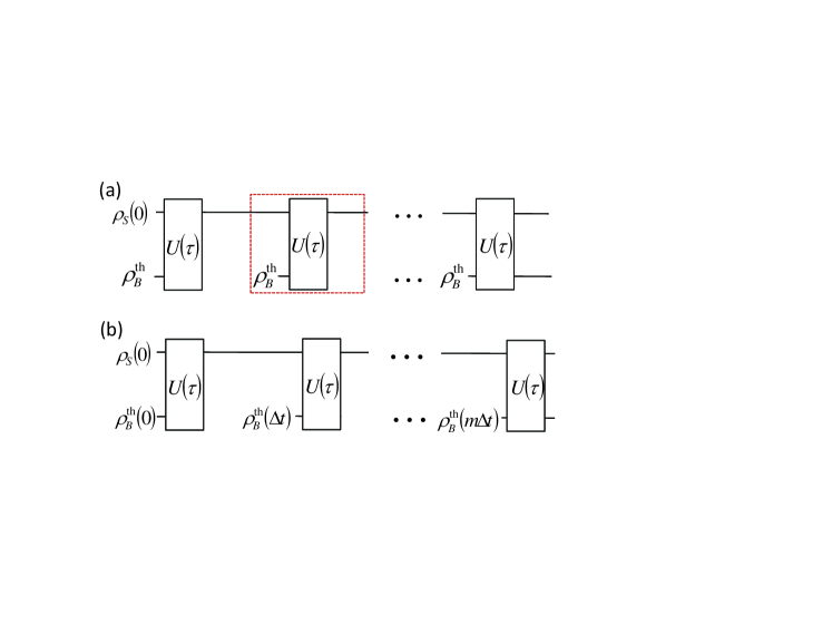
Figure 1: (a) Quantum circuit for simulating the Markovian dynamics of an open quantum system coupled to a time-independent environment. The first register represents the open system and the second register represents the environment. (b) Quantum circuit for simulating the Markovian dynamics of an open system coupled to a time-dependent environment.

The large size of the environment plays a crucial role in justifying the Markovian approximation. Under this approximation, the typical time during which the internal correlations of the environment related to the effects of the open system exist, $\tau_{R}$, is much shorter than the characteristic relaxation time of the open system, $\tau_{S}$; as a result, the influence of the open system on the environment is small and can be ignored. Therefore, the state of the global system at any time $t$ can be approximately described by the tensor product breuer1

$$\rho(t)\approx\rho_{S}(t)\otimes\rho_{B}^{\text{th}}.$$ (18)

where $\rho_{B}^{\text{th}}$ is the thermal equilibrium state of the environment and can be written as

$$\rho_{B}^{\text{th}}=\sum_{j}P_{j}|j\rangle\langle j|,j=1,\cdots,L=2^{d},$$ (19)

with

$$P_{j}=\frac{e^{-\beta E_{j}}}{Z},$$ (20)

and $|j\rangle$ ($E_{j}$) are the eigenvectors (eigenvalues) of the environment Hamiltonian $H_{B}$, $Z$ is the partition function

$$Z=\sum_{j=1}^{L}e^{-\beta E_{j}},$$ (21)

where $\beta=1/k_{B}T$, $k_{B}$ is the Boltzmann constant and $T$ is the temperature. Note that in the absence of interactions between the environment qubits, the eigenstates $|j\rangle$ can be written as a tensor product of the states of the environment qubits

$$|j\rangle=|j_{1}\rangle\otimes|j_{2}\rangle\otimes\cdots\otimes|j_{d}\rangle,$$ (22)

and the eigenvalues $E_{j}$ can be written as a sum of the eigenvalues of the Hamiltonians of the environment qubits for the corresponding eigenstate $|j\rangle$

$$E_{j}=E\left(j_{1}\right)+E\left(j_{2}\right)+\cdots+E\left(j_{d}\right).$$ (23)

As a result, the thermal-equilibrium state of the environment is a tensor product of the thermal-equilibrium states of the individual qubits:

$$\rho_{B}^{\text{th}}=\rho_{1}^{\text{th}}\otimes\rho_{2}^{\text{th}}\otimes\cdots\otimes\rho_{d}^{\text{th}},$$ (24)

where

$$\rho_{k}^{\text{th}}=\left(1-p_{k}\right)|0\rangle\langle 0|+p_{k}|1\rangle\langle 1|,$$ (25)

denotes the thermal equilibrium state of the $k$-th environment qubit and

$$p_{k}=\frac{1}{1+e^{\beta\omega_{k}}}.$$ (26)

An alternative method that can be used to obtain the Markovian approximation for a relatively small environment is to frequently force it back into its thermal-equilibrium state. This process can be implemented relatively easily on a quantum computer, where one has full access to all the qubits. The procedure for simulating the Markovian dynamics of the open system is therefore as follows: Set the environment to its thermal equilibrium state, couple the open system to the environment modes and let the global system evolve for some time, then reset the state of the environment to its thermal equilibrium state. Repeat this process many times and then read out the state of the open system. Mathematically, the evolution of the open system in one step is expressed as

$$\rho_{S}^{\left(j+1\right)}\left[(j+1)\tau\right]=\text{Tr}_{B}\left[U(\tau)\rho^{j}(j\tau)U^{{\dagger}}(\tau)\right],j=0,1,2,\dots$$ (27)

where $\rho^{j}(j\tau)=\rho_{S}^{j}\otimes\rho_{B}^{th}$.

Based on the above analysis, the evolution of the open system can be simulated as follows on a quantum computer $\left[\text{see Fig.}~{}1\left(a\right)\right]$: prepare two quantum registers $R_{S}$ and $R_{B}$ to represent the open system and the environment, respectively;

$\left(i\right)$ on the quantum register $R_{S}$, prepare the initial state of the open system;

$\left(ii\right)$ on the quantum register $R_{B}$, prepare the thermal equilibrium state of the environment;

$\left(iii\right)$ implement the unitary operation $U(\tau)=\exp(-iH\tau)$ on the registers $R_{S}$ and $R_{B}$, where $H$ is the model Hamiltonian;

$\left(iv\right)$ repeat steps $\left(ii\right)-\left(iii\right)$ a number of times.

$\left(v\right)$ read out the state, or the desired observable, of the register $R_{S}$.

In general, the different terms in the model Hamiltonian do not commute. We therefore employ the Trotter-Suzuki formula nc for implementing the unitary operation $U(\tau)=\exp(-iH\tau)$

$$U(\tau) = \exp\left[-iH\tau\right]$$ (28)

$$= \lim_{n\rightarrow\infty}\left[e^{-iH_{S}\tau/n}e^{-iH_{B_{1}}\tau/n}e^{-iH_{I_{1}}\tau/n}\cdots e^{-iH_{B_{d}}\tau/n}e^{-iH_{I_{d}}\tau/n}\right]^{n}$$

$$= \lim_{n\rightarrow\infty}\left[U_{S}\left(\tau/n\right)U_{B_{1}}\left(\tau/n\right)U_{I_{1}}\left(\tau/n\right)\cdots U_{B_{d}}\left(\tau/n\right)U_{I_{d}}\left(\tau/n\right)\right]^{n}$$

$$\approx \left[U_{S}\left(\tau/n_{0}\right)U_{B_{1}}\left(\tau/n_{0}\right)U_{I_{1}}\left(\tau/n_{0}\right)\cdots U_{B_{d}}\left(\tau/n_{0}\right)U_{I_{d}}\left(\tau/n_{0}\right)\right]^{n_{0}},$$

where $n_{0}$ is a finite but large number.

In many cases, one is interested in the value of some physical properties of the open system in the thermal-equilibrium state, such as various correlation functions, the partition function, etc. The thermal equilibrium state of the open system can be obtained by repeating the steps $\left(ii\right)-\left(iii\right)$ until the open system reaches its thermal equilibrium state terhal .

Note that the steps followed in implementing the algorithm explained above are the same as those used in the algorithm of Ref. terhal . The goal of that work, however, is different from the goal of our work. Our algorithm simulates the dynamics whereas the algorithm of Ref. terhal aims to prepare the thermal equilibrium state of the system. This difference in the purpose of the algorithm leads to a number of further differences. For example, in our case, we have to design the interaction Hamiltonian and the parameters of the environment such that we accurately reproduce the spectral density of the environment. In Ref. terhal , one only requires that certain inequalities are satisfied in order for the environment register to act as a good environment. In other words, the exact speed of reaching thermal equilibrium is not a crucial issue in that work, as long as the thermal-equilibrium state is reached in polynomial time. In contrast, if for example there is some symmetry in the simulated system that prevents it from reaching the thermal-equilibrium state, then our algorithm would still be considered to work successfully if it produces the correct dynamics, even though the thermal-equilibrium state is never reached.

II.2.1 Timescales

At this point we should make a few comments regarding the time scales involved in applying the algorithm. The time interval $\tau$ should be very short compared with $\tau_{S}$ (so that the state of the open system changes slightly during $\tau$). The time $\tau$ can be considered the memory time of the environment since the environment is reset to its thermal equilibrium state at every time interval $\tau$. Since the timescale for dynamics involving the system and a resonant mode of the environment is given by the inverse of $c_{i}$ times a matrix element between energy eigenstates of the system, the Markovian condition would require that $\tau$ must be small compared to this timescale, such that that the change in the system’s density matrix is small during the time $\tau$. When constructing the model Hamiltonian, the frequency spectrum of the environment is discretized into many elements where each element has a width $\Delta\omega$. This width $\Delta\omega$ must be at most on the order of $1/\tau$ to make sure that the different $\delta$-peaks have large overlap and produce a smooth spectral density since the width of the $\delta$-peaks is on the order of $1/\tau$.

Note that our algorithm can be straightforwardly generalized to simulate the Markovian dynamics of an open system coupled to a time-dependent environment [see Fig. $1\left(b\right)$]. In each iteration, the state of the environment register is reset to the time-dependent thermal equilibrium state of the time-dependent environment. The algorithm can also be generalized for the case of an open system that is simultaneously coupled to two or more different environments with different temperatures.

II.2.2 Sequential application of the different dissipation channels

In the above procedure for simulating the dynamics of an open quantum system, we have assumed that each mode in the environment is represented by one qubit. In the quantum circuit shown in Fig. $1\left(a\right)$, the environment quantum register $R_{B}$ is prepared in the thermal equilibrium state of all the environment qubits with all the different frequencies. The operator $U(\tau)$ acts in the state space of the system qubits and all the environment qubits.

In this subsection, we show that one can reduce the number of qubits required to represent the environment by having each qubit represent multiple environment modes. In this approach each “evolve-reset”step in the algorithm above is split into multiple evolve-reset steps, and in each one of those steps a qubit represents one environment mode. However, the qubit is reset to different frequencies in the different steps such that it produces the effect of multiple environment modes on the system. Under certain conditions even a single qubit can be used to represent the entire environment: the parameters of this qubit are sequentially alternated between several different settings such that the sequence covers all the dissipation channels of the environment.

In the master equation shown in Eq. ($3$), the derivative of the reduced density matrix of the open system is described by a sum over the decay processes of the open system through all the different dissipation channels. In the simulation algorithm, the decay of the open system in one step of the evolution can be expressed as

$$\rho_{S}^{\text{int}}\bigl{[}(j+1)\tau\bigr{]} = \text{Tr}_{B}\Bigl{\{}U^{\text{int}}(\tau)\bigl{[}\rho_{S}(j\tau)\otimes\rho_{B}^{th}\bigr{]}U^{\text{int}{\dagger}}(\tau)\Bigr{\}}$$ (29)

$$= \left(1-\tau\varGamma\right)\rho_{S}^{\text{int}}(j\tau),$$

where $\varGamma$ is a superoperator that describes the decay of the open system and it is a sum over the contributions from all the different environment modes (the superscript “int” indicates the interaction picture). Let $\varGamma_{j}$ denote the superoperator that describes the decay of the open system caused by the coupling of the open system to only the $j$-th environment mode. If the open system undergoes a small change during the time $\tau$, such that $\tau\varGamma\ll 1$ (i.e., all the eigenvalues of $\varGamma$ times $\tau$ are much smaller than $1$), then the evolution of the open system can be approximated as

$$1-\tau\varGamma\approx\left(1-\tau\varGamma_{1}\right)\left(1-\tau\varGamma_{2}\right)\cdots\left(1-\tau\varGamma_{d}\right).$$ (30)

Therefore, the decay of the open system can be simulated by applying the environment modes to the open system sequentially.

As a result, an alternative approach for simulating the dynamics of an open system goes as follows: We divide the environment modes into a few sets and let the different sets interact with the open system sequentially. In this way, we effectively simulate the interaction between the open system and all the different modes in the environment. The Hamiltonian for the open system interacting with the $i$-th set of the environment modes is given by

$$H^{\left(i\right)}=H_{S}+\sum_{k=1}^{d_{i}}H_{B_{k}}^{\left(i\right)}+\sum_{k=1}^{d_{i}}H_{I_{k}}^{\left(i\right)},$$ (31)

where $i=1,2,\cdots,d/d_{i}$ and $d_{i}$ is the number of the environment modes in each set.

One point that requires a little bit extra care here is that each mode in the environment is coupled to the system in only one step out of $d/d_{i}$ steps, whereas the system Hamiltonian $H_{S}$ is applied in all of the steps. One therefore needs to be careful how to calculate the elapsed time in the simulated system. If the Hamiltonian in Eq. ($31$) is applied with a given value of $\tau$, then after covering all the $d/d_{i}$ sets of environment modes the system Hamiltonian would have induced a change corresponding to a time $\tau\times d/d_{i}$, while each environment mode would have induced a change corresponding to a time $\tau$. In order to avoid any problems arising from this inconsistency, one can note that decoherence rates are proportional to the spectral density (and therefore proportional to $c_{i}^{2}$) from the interaction Hamiltonian. One can then use a rescaled Hamiltonian

$$\widetilde{H}^{{}^{\left(i\right)}}=H_{S}+\sum_{j=1}^{d_{i}}H_{B_{j}}^{\left(i\right)}+\sqrt{\frac{d}{d_{i}}}\sum_{j=1}^{d_{i}}H_{I_{j}}^{\left(i\right)}.$$ (32)

If this Hamiltonian is now applied for a time $\tau$, then after covering all the different environment modes both the system Hamiltonian and the coupling to the environment would have induced changes that correspond to a time $\tau\times d/d_{i}$, removing the inconsistency in the elapsed time. Note that in order to guarantee the validity of the Markovian approximation, the rescaled coupling strengths $c_{i}\times\sqrt{d/d_{i}}$ must still be small compared to $1/\tau$.

The new procedure for simulating the Markovian dynamics of open systems is implemented on a quantum computer as follows:

$i)$ on the quantum register $R_{S}$, prepare the initial state of the open system;

$ii)$ on the quantum register $R_{B}$, prepare the thermal equilibrium state of the qubits representing a subset of the environment modes;

$iii)$ implement the unitary operation $U_{i}(\tau)=\exp\left[-i\widetilde{H}^{{}^{\left(i\right)}}\tau\right]$ on the registers $R_{S}$ and $R_{B}$;

$iv)$ perform steps $ii)-iii)$ for another set of environment modes, and keep repeating this process until the algorithm runs over all the sets of the environment modes;

$v)$ repeat steps $ii)-iv)$ a number of times;

$vi)$ read out the state, or the desired observable, of the register $R_{S}$;

In Eq. ($30$), the error in the decay of the open system introduced by sequentially applying the dissipation channels, up to second order in $\tau$, is $\tau^{2}\sum_{i,j}\varGamma_{i}\varGamma_{j}$. In the case of using only a single qubit to represent the environment, the algorithm will have an error of $d^{2}\tau^{2}\overline{\varGamma}_{0}^{2}$, where $\overline{\varGamma}_{0}$ denotes the overall scale of the decay rate of the open system caused by the coupling of the open system to a single environment mode. When $d$ is large, this approximation can introduce a large error. On the other hand, if we use more qubits to represent the environment, the errors will be smaller because there will be fewer terms in the sum for the error.

II.3 State preparation and readout

In the algorithm, the initial state of the global system is set to $\rho_{S}(0)\otimes\rho_{B}^{\text{th}}$, where $\rho_{S}(0)$ is the initial state of the open system and $\rho_{B}^{\text{th}}$ represents the thermal equilibrium state of the environment. To prepare the initial state of the global system on a quantum computer, we prepare two quantum registers $R_{S}$ and $R_{B}$ to represent the open system and the environment, respectively. In general, the thermal equilibrium state of the environment is a mixed state. In order to prepare the mixed state $\rho_{B}^{\text{th}}$ as shown in Eq. ($19$), we can generate a random integer $j$, where $j\in\left[1\text{, }L\right]$, with probability $P_{j}$. Then we prepare the corresponding state $|j\rangle$ on the quantum register $R_{B}$. We repeat this step many times. This procedure produces an ensemble (in time) of states $|j\rangle$ with the corresponding probabilities $P_{j}$. This ensemble gives the same effect as the case where the quantum register $R_{B}$ is prepared in a thermal equilibrium state in every time step.

As discussed in subsection II.A, in the absence of interactions between the environment qubits, the thermal-equilibrium state of the environment is a tensor product of the thermal-equilibrium states of the individual qubits as shown in Eq. ($24$). In such cases, the thermal-equilibrium state of the environment can be prepared in a simpler way: randomly generating $0$ or $1$ with respective probabilities $\left(1-p_{k}\right)$ and $p_{k}$, then preparing the corresponding states $|0\rangle$ or $|1\rangle$ on the environment qubit, and repeating this step many times, the mixed state $\rho_{B}^{\text{th}}$ can be prepared. In this procedure, an ensemble (in time) of states $|0\rangle$ and $|1\rangle$ with the corresponding probabilities $p_{k}$ and $\left(1-p_{k}\right)$ is produced, and it gives the same effect as the case where the environment qubit is prepared in a thermal equilibrium state in every time step.

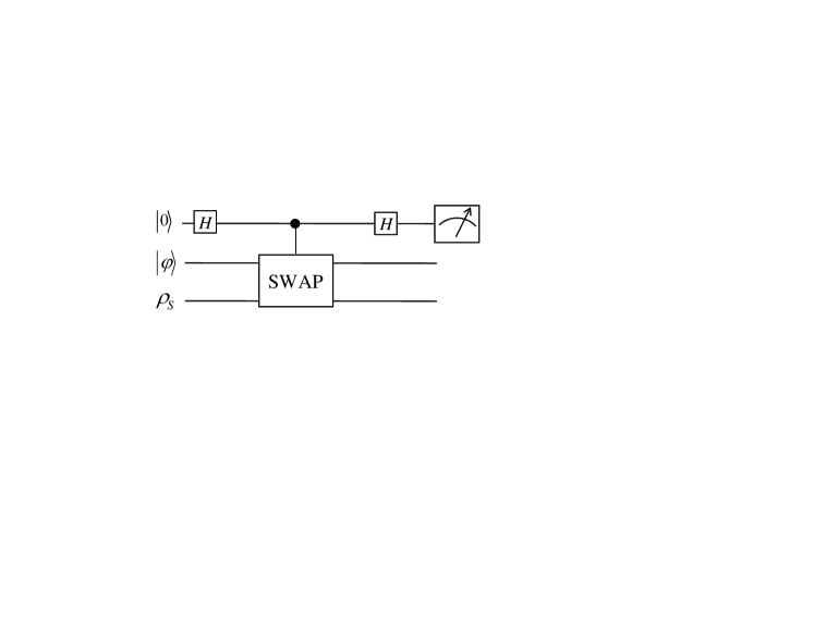
Figure 2: Quantum circuit for a quantum estimator. $H$ represents the Hadamard gate and SWAP represents the swap gate.

Observing the decoherence dynamics can be performed in a number of different ways. For example, the phase estimation procedure nc can be used to measure the energy of the open system, and one can then monitor the dynamics of the energy distribution.

Alternatively, any matrix element in the density matrix of the open system can be obtained using a quantum estimator ekert ; horodecki as shown in Fig. $2$. In the circuit for the quantum estimator, if we prepare the second register in the state $|\varphi\rangle$ and the third register in the state $|\psi\rangle$, then the value of $|\langle\varphi|\psi\rangle|$ can be estimated by performing single-qubit measurements on the index qubit. Through some derivation ekert we have

$$P\left(0\right)=\frac{1}{2}\left(1+|\langle\varphi|\psi\rangle|^{2}\right),$$ (33)

where $P\left(0\right)$ is the probability for obtaining the state $|0\rangle$ in the index qubit. If the third register is in a mixed state $\rho_{S}$, then we have

$$P\left(0\right)=\frac{1}{2}\left(1+\langle\varphi|\rho_{S}|\varphi\rangle\right).$$ (34)

For the readout of the state of the open system in some chosen basis $\{|n\rangle\}$, any diagonal element $\rho_{nn}^{S}=\langle n|\rho_{S}|n\rangle$ can be estimated by preparing the second register in the state $|n\rangle$ and the third register in the state $\rho_{S}$. For the off-diagonal elements $\rho_{mn}^{S}=\langle m|\rho_{S}|n\rangle$, the real part of $\rho_{mn}^{S}$ can be estimated by preparing the second register in the state $|\varphi\rangle=\left(|m\rangle+|n\rangle\right)/\sqrt{2}$. The imaginary part of $\rho_{mn}^{S}$ can be estimated by setting $|\varphi\rangle=\left(|m\rangle+i|n\rangle\right)/\sqrt{2}$.

The circuit shown in Fig. $2$ can also be used for evaluating the expectation values of arbitrary observables. For an operator $F$, by applying the technique developed in Refs. ekert ; horodecki , one can obtain the value of $\langle F\rangle_{\rho_{S}}$. Then combined with the quantum circuit for simulating the Markovian dynamics of open systems, one can simulate the evolution of the expectation values of the physical observables. Various correlation functions can also be obtained using this technique.

II.4 Simulating pure dephasing of a quantum system

So far we have concentrated on the case where the nonunitary part of the dynamics is caused by the environment modes that are resonant with the open system. This picture is valid for energy relaxation. Pure dephasing, on the other hand, is caused by low-frequency noise. Such low-frequency noise can also be generated using the algorithm explained in the previous subsections: whenever an environment qubit’s state is changed from the ground to the excited state or vice versa, the open system feels a telegraph-noise-like change. This telegraph noise then causes (mostly) pure dephasing in the system. Although this effect can be induced using environment qubits, there is a simpler method to generate telegraph noise. The telegraph noise is essentially a classical noise signal affecting the open system. There is therefore no need to use qubits in order to produce this classical signal. It can be generated using a classical algorithm and added to the system Hamiltonian $H_{S}$. If different noise signals are used in the different runs of the algorithm, the density matrix of the system (averaged over the different realizations) will exhibit dephasing dynamics as a function of time.

For an open system coupled to many fluctuators, the Hamiltonian for the system can be expressed as gal  [see Eq. ($11$) for comparison]

$$H=H_{S}+\sum_{k}\chi\!_{k}\left(t\right)\widetilde{A}_{k},$$ (35)

where

$$\ \chi_{k}\left(t\right)=\sum_{i}v_{ik}\;\xi_{ik}\left(t\right),$$ (36)

the random functions $\xi_{i}\left(t\right)$ characterize the fluctuators’ state, instantly switching between $\pm 1/2$ at random times. Therefore, the simulation of the open system coupled to a bath of many fluctuators is reduced to simulating a closed quantum system, which will reduce the resources required for performing the simulation.

In simulating the dynamics of a quantum system coupled to many fluctuators, we prepare the initial state of the system on a quantum register, then implement the unitary operation $U=\exp\left(-iH\tau\right)$. Since the signal $\chi\left(t\right)$ is random, to obtain the evolution of the quantum system, we have to run the algorithm many times with a different signal $\chi\left(t\right)$ in each run.

The noise spectrum of a noise signal is defined as ymg

$$s\left(\omega\right)=\frac{1}{\pi}\int_{0}^{\infty}\!\!dt\;\cos\omega t\langle\chi\left(t\right)\chi\left(0\right)\rangle.$$ (37)

In order to generate the telegraph-noise signal kog , we assume that the environment contains a number of fluctuators. Each fluctuator switches between two possible configurations with switching rate $\gamma_{i}$, and couples to the system with a coupling strength $v_{i}$. The corresponding contribution of a fluctuator to the noise spectrum is a Lorentzian ymg ,

$$s_{i}\left(\omega\right)=\frac{v_{i}^{2}\gamma_{i}}{4\pi\left(\omega^{2}+\gamma_{i}^{2}\right)}.$$ (38)

The (low-frequency) noise spectrum of the entire environment is the sum of the noise spectra of all the fluctuators

$$S\left(\omega\right)=\sum_{i}\frac{v_{i}^{2}\gamma_{i}}{\omega^{2}+\gamma_{i}^{2}}.$$ (39)

By adjusting the parameters $\gamma_{i}$ and $v_{i}$, one can produce a variety of noise spectra. A typical example in practical situations is $1/f$ noise. If the number and density of fluctuators is sufficiently large, and the distribution of the switching rates of the fluctuators $D\left(\gamma\right)\propto\gamma^{-1}$, and is independent of the distribution of the coupling strengths between the fluctuators and the open system, the sum over the fluctuators produces the $1/f$ noise spectrum dutta

$$S\left(\omega\right)=\frac{G}{\omega},$$ (40)

where $G$ is a constant.

II.5 Simulating the non-Markovian dynamics of an open system

The quantum algorithm presented above for simulating the Markovian dynamics of an open system can also be used for simulating a class of non-Markovian dynamics of open systems. A common situation where non-Markovian dynamics occurs is the case where a small number of degrees of freedom in the environment are coherent enough that they have non-negligible memory effects in their interaction with the open system breuer1 . Examples of this situation include the relaxation dynamics of an atom through a cavity that has a high quality factor (see e.g., Ref. breuer1 ) and the relaxation dynamics of a superconducting qubit close to resonance with a coherent two-level defect (see e.g. Ref. ashhab ).

When a small number of degrees of freedom in the environment are responsible for the non-Markovian dynamics, and assuming that one has sufficient understanding of these degrees of freedom (i.e. their intrinsic Hamiltonian, their coupling to the system and their decoherence mechanisms and rates), it becomes relatively straightforward to include them in the algorithm. One now adds the appropriate number of ancilla qubits needed to describe these degrees of freedom. When implementing the evolve-reset part of the algorithm, one treats the additional degrees of freedom as part of the system, i.e. they are not reset to their initial state. When the measurement is performed at the end of the algorithm, however, only the system qubits are used and the additional degrees of freedom are ignored. This step corresponds to taking the trace over the state of these degrees of freedom.

The introduction of the additional degrees of freedom increases the resource requirements (which will be the subject of Sec. III) as follows: the number of qubits used in implementing the unitary operation $U(\tau)$ is increased by $\log(D_{\text{ext}})$, where $D_{\text{ext}}$ is the number of degrees of freedom in the environment that are responsible for the non-Markovian dynamics. Since the interactions in the expanded system should still be local, the scaling of resources will still be polynomial in system+ancilla size and therefore efficient.

II.6 Implementing environments other than spin baths

Our algorithm simulates the effect of the environment using a set of ancilla qubits that each represents one spin in a bath of independent spins pro . This type of environment is rather straightforward to implement, since the properties and manipulation of the environment are done by considering the ancilla qubits one at a time. For a variety of purposes, this spin bath is sufficient for the implementation of the desired quantum simulation. However, the spin bath has certain limitations. For example, the two-level nature of the environment elements (i.e., spins) means that increasing the temperature will reduce the number of spins that are in their ground states, thus reducing the relaxation rate induced by this environment lidar . This behavior contrasts with the case of a bath of harmonic oscillators, where both relaxation and excitation rates increase with increasing temperature. Therefore, if one is interested in the temperature dependence of the dynamics, one needs to be careful about the differences between different types of environments.

One possible technique to use a spin bath in order to simulate an oscillator bath and obtain the correct temperature dependence is to calculate a modified (temperature-dependent) spectral density for the spin bath and use this spectral density in the simulation. Alternatively, different types of environments can be simulated by modifying the algorithm such that each element in the environment is encoded into multiple qubits that are treated as a single physical object. For example, one could use $n$ environment qubits to represent the lowest $2^{n}$ energy levels of a harmonic oscillator and then design a Hamiltonian where this harmonic oscillator represents one mode in the environment. Thus, one can simulate the dynamics of an open quantum system interacting with a bath of harmonic oscillators. Note that the state preparation and the form of the Hamiltonian become more complicated in this case than in the case of a spin bath.

III Resource estimation

In this section, we discuss the resources including the number of qubits and the operations needed for implementing the algorithm.

As shown in Fig. $1\left(a\right)$, the number of qubits required for simulating the Markovian dynamics of the open system is $\lceil\log_{2}N\rceil+d$ (here $\lceil x\rceil$ provides the smallest integer larger than $x$, or equal to $x$ if $x$ is an integer), where $N$ is the dimension of the Hilbert space of the open system and $d$ is the total number of qubits representing the environment. In the quantum estimator for the readout of the state of the open system, $\lceil\log_{2}N\rceil+1$ additional qubits are needed as shown in Fig. $2$. Therefore the total number of qubits for simulating the Markovian dynamics of open systems is $2\lceil\log_{2}N\rceil+d+1$. One could also use the ancilla qubits that are used in representing the environment in the readout of the state of the open system, which would reduce the number of qubits used in the algorithm to $\max\left[\lceil\log_{2}N\rceil+d,2\lceil\log_{2}N\rceil+1\right]$.

Table 1: Resource needed for implementing the algorithm. Here $\lceil x\rceil$ provides the smallest integer larger than $x$, or equal to $x$ if $x$ is an integer. $N$ is the dimension of the Hilbert space of the open system, $d$ is the total number of qubits needed in representing the environment in one time, $d_{i}$ is the number of qubits used in representing the environment in approach $2$. $m$ is the number of times the unitary operation $U(\tau)=\exp(-iH\tau)$ is implemented, and $n_{0}$ is the parameter for dividing the time in the Trotter expansion in Eq. ($28$).

Algorithm		# of qubits		# of operations
Approach $1$		$2\lceil\log_{2}N\rceil\!+\!d\!+\!\!1$		$O(m\!\times\!\left(2d+1\right)^{n_{0}})$
Approach $2$		$2\lceil\log_{2}N\rceil\!+\!d_{i}\!+\!\!1$		$O(m\!\times\!d/d_{i}\!\times\!\left(2d_{i}+1\right)^{n_{0}})$

The unitary operation $U(\tau)=\exp(-iH\tau)$, where $H$ is the model Hamiltonian, is implemented a finite number $m$ of times. To implement $U(\tau)$ on the quantum circuit, we employ the Trotter-Suzuki formula as shown in Eq. ($28$), in which $U(\tau)$ is approximated by the product of $\left(2d+1\right)^{n_{0}}$ unitary transformations, where $n_{0}$ is the parameter for dividing the time in the Trotter expansion. Therefore the number of unitary operations needed in the quantum circuit shown in Fig. $1\left(a\right)$ is $m\times\left(2d+1\right)^{n_{0}}$. Note one could obtain higher efficiency using higher order Suzuki-Trotter formulas, as discussed in Ref. childs

In the second approach we presented, the environment is represented using a few or a single qubit. The number of qubits required for simulating the dynamics of open systems is: $2\lceil\log_{2}N\rceil+d_{i}+1$, where $d_{i}$ is the number of qubits representing the environment.

The unitary operations implemented for each set of qubits are $U_{i}(\tau)=\exp\left[-i\widetilde{H}^{{}^{\left(i\right)}}\tau\right]$, where $\widetilde{H}^{{}^{\left(i\right)}}$ is given in Eq. ($32$). Thus implementing $U_{i}(\tau)$ on the circuits by employing the Trotter-Suzuki formula requires $\left(2d_{i}+1\right)^{n_{0}}$ unitary operations. For $d/d_{i}$ sets of the environment elements where each set of the elements is implemented $m$ times, the total number of unitary operations that need to be implemented is $m\times d/d_{i}\times\left(2d_{i}+1\right)^{n_{0}}$.

In preparing the initial state of the global system, we have to prepare the thermal equilibrium state of the environment, which is a mixed state, a number of times. To prepare the thermal equilibrium state $\rho_{B}^{th}$ as shown in Eq. ($19$), we prepare the state $|j\rangle$ with the corresponding probability $P_{j}$, and repeat this step many times. In running the algorithm, these basis states are fed to the register $R_{B}$ in the quantum circuit in Fig. $1\left(a\right)$ one at a time, and run the algorithm many times with the the register $R_{B}$ prepared in the basis states. For each basis state $|j\rangle$, we need to reset the state on the register $R_{B}$ $m$ times in the algorithm. To do this, we need to erase the state on the register $R_{B}$ and then prepare $R_{B}$ in state $|j\rangle$. We can first perform a measurement on the register $R_{B}$, the state on $R_{B}$ collapse to a basis state, then we can perform a unitary operation to rotate this state into the state $|j\rangle$.

In the readout of the state of the open system, we employ the quantum estimator, in which the information of the open system is obtained by performing single-qubit measurements on the index qubit and taking the average. We have to prepare many copies of the state of the open system in order to obtain accurate results. Both this procedure and the procedure for preparing the thermal equilibrium state of the environment require running the algorithm many times. The number of times for running the algorithm, however, does not depend on the dimension of the Hilbert space of the open system. Therefore the algorithm can be implemented efficiently using $O\left[m\times\left(2d+1\right)^{n_{0}}\right]$ (or $O\left[m\times d/d_{i}\times\left(2d_{i}+1\right)^{n_{0}}\right]$, if the environment is represented using $d_{i}$ qubits) unitary operations. All these results are summarized in Table I.

IV Example: a two-level system in a spin bath

In this subsection, we consider the example of simulating the Markovian dynamics of a two-level system that is immersed in a thermal bath of independent two-level systems. The Hamiltonian of the global system is given by

$$H=-\frac{1}{2}\,\omega_{s}\,\sigma^{z}-\frac{1}{2}\sum_{k}\omega_{k}\,\sigma_{k}^{z}+\frac{1}{2}\sigma^{x}\otimes\sum_{k}c_{k}\,\sigma_{k}^{x},$$ (41)

where $\sigma^{x}$ and $\sigma^{z}$ are the Pauli operators, and $\omega_{s}$ and $\omega_{k}$ are the frequencies of the two-level system and the environment modes, respectively. The first term is the Hamiltonian of the open system, the second term is the Hamiltonian of the environment and the third term describes the interaction between the open system and the environment.

In this example, assuming Ohmic dissipation, the spectral density of the spin bath is expressed as hanggi

$$J\left(\omega\right)=2\pi\alpha\omega\exp\left(-\omega/\omega_{c}\right),$$ (42)

where $\alpha$ is the dissipation coefficient and $\omega_{c}$ denotes the cutoff frequency ($\omega_{c}/\omega_{s}\gg 1$). Below we specify frequencies, temperatures and times using a standard unit frequency $\Delta_{0}$. We first set $\omega_{s}/\Delta_{0}=1$, $\alpha=2\times 10^{-4}$, $\omega_{c}/\Delta_{0}=100$, and $\beta\Delta_{0}=1$. The frequency spectrum in the region $\omega/\Delta_{0}\in\left[0.8\text{, }1.15\right]$ is discretized into eight elements at frequencies $\omega_{k}/\Delta_{0}=\left(0.80+0.05k\right)$, with $k=0$, $1$, $\cdots 7$. The width of each element is $\Delta\omega/\Delta_{0}=0.05$. The coupling coefficients $c_{k}$ are determined using Eq. ($14$).

For this example, the analytical results for the relaxation rate and the dephasing rate, $1/T_{1}$ and $1/T_{2}$, can be derived under the Markovian approximation cohen as

$$\frac{1}{T_{1}}=\frac{1}{2}J\left(\omega=\omega_{s}\right),\text{ \ \ \ \ }\frac{1}{T_{2}}=\frac{1}{2T_{1}}.$$ (43)

The Markovian dynamics of the two-level system is simulated with the initial state of the open system being set to the excited state $|e\rangle$ of the two-level system. We set the unitary evolution time $\Delta_{0}\tau=30$, and we obtain the evolution of the state of the open system. The relaxation dynamics of the two-level system is shown in Fig. $3$.

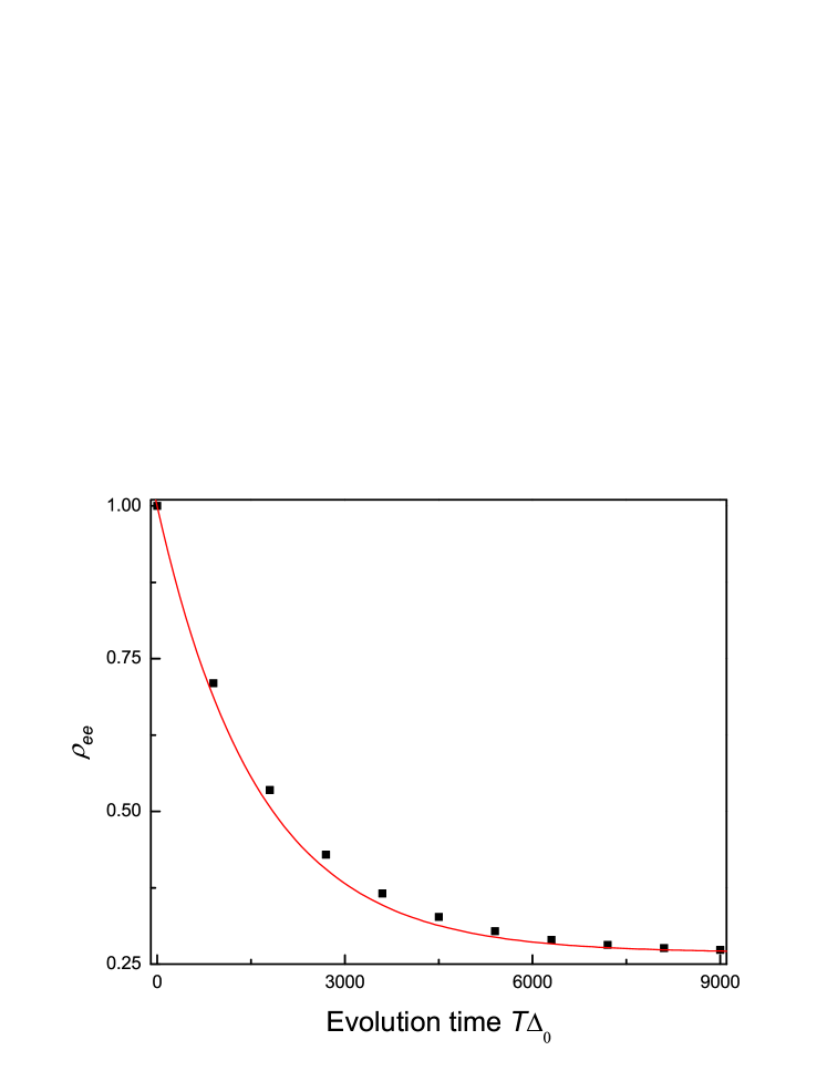
Figure 3: (Color online) The evolution of the matrix element $\rho_{ee}$ of a two-level system in a spin bath, where $\rho_{ee}$ denotes the diagonal element of the density matrix that describes the population of the excited state. The frequency of the environment mode in the region $\omega/\Delta_{0}\in\left[0.8\text{, }1.15\right]$ is divided into $8$ elements with equal width and each element is represented by a qubit. The Hamiltonian for the global system is given by Eq. ($41$). The unitary evolution time $\Delta_{0}\tau=30$. The red solid line represents the analytical result for the evolution of $\rho_{ee}$ with the initial state $|e\rangle$. The black square dots represent the simulated results for the evolution of $\rho_{ee}$.

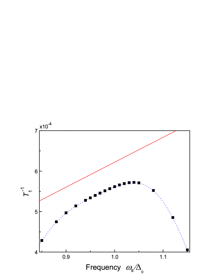
Figure 4: (Color online) The relaxation rate of the two-level system as a function of its frequency. The black squares represent the results obtained from the simulation of the algorithm; the blue dotted line represents the relaxation rate obtained by using the spectral density that is spanned by eight $\delta$-peaks in Eq. ($44$); and the red solid line represents the relaxation rate obtained from the analytical spectral density in Eq. ($42$). Obviously only the first two ones agree well with each other.

Figure 5: (Color online) The relaxation rate of the two-level system as a function of the frequency of the two-level system. The black square dots represent the results obtained from the simulation of the algorithm using the improved coupling coefficients as discussed in the text; the blue dotted line represents the relaxation rate obtained by using the spectral density that is produced by eight $\delta$-peaks in Eq. ($44$) using the improved coupling coefficients; and the red solid line represents the relaxation rate obtained from the analytical spectral density in Eq. ($42$).

From Fig. $3$, we can see that there is a clear discrepancy between the relaxation rates obtained from the numerical simulation and the exact results given by Eq. ($43$). This discrepancy is due to the fact that we used Eq. ($14$) to determine the coupling coefficients $c_{k}$ even though only eight $\delta$-peaks are used to represent the spectral density:

$$J\left(\omega\right)=\pi\sum_{k=1}^{k=8}c_{k}^{2}\;\delta\left(\omega-\omega_{k}\right).$$ (44)

Each $\delta$-peak has the analytical form terhal

$$\delta\left(\frac{\omega-\omega_{0}}{\Delta_{0}},\tau\Delta_{0}\right)=\frac{1-\cos[\tau\left(\omega-\omega_{0}\right)]}{\pi\tau\Delta_{0}\left[(\omega-\omega_{0})/\Delta_{0}\right]^{2}}.$$ (45)

In Eq. ($14$), a good approximation can be achieved when many $\delta$-peaks are used to represent the spectral density and the peaks cover a sufficiently wide range of frequencies. The eight peaks used in our simulation do not satisfy these conditions.

In order to further demonstrate the above explanation of the discrepancy, in Fig. $4$ we show the relaxation rate as a function of the frequency $\omega_{s}$ of the two-level system. There we compare the numerical results obtained from the simulation, the analytical results obtained from Eq. ($43$) with the spectral density given by Eqs. ($44$) and ($45$) and the coupling coefficients determined through Eq. ($14$); and the exact results obtained from Eq. ($43$) with the spectral density given by Eq. ($42$). From Fig. $4$ we can see that the numerical results for the relaxation rate obtained from the simulation fit very well the analytical results of the eight-peak spectral density, while both have a systematic deviation from the exact results.

Table 2: Results for simulating the Markovian dynamics of a two level system using different number of qubits to represent the environment to sequentially simulate a total of eight dissipation channels. $N$ denotes the number of qubits representing the environment modes. The exact result for $T_{1}$ is $T_{1}^{\text{exact}}=2/J(\omega=\Delta_{0})$, and $T_{2}^{\text{exact}}=2T_{1}$. The results here are obtained using the improved choice of the coupling coefficients as discussed in the text. The results are essentially independent of $N$.

$N$		$1$		$2$		$4$		$8$
$T_{1}/T_{1}^{\text{exact}}$		$0.998$		$0.998$		$0.998$		$0.996$
$T_{2}/T_{1}^{\text{exact}}$		$1.994$		$1.990$		$1.991$		$1.991$

This systematic deviation from the exact results can be eliminated by plugging in the analytical form of the $\delta$-peaks as shown in Eq. ($45$) into Eq. ($44$) for the eight elements and then obtaining an improved approximation for the coupling coefficients $c_{k}$. In Fig. $5$, we show the relaxation rate as a function of the frequency of the two-level system using the improved choice of the coupling coefficients. One can see that in the region around $\omega_{s}/\Delta_{0}=1.0$, the numerical results are now in good agreement with the exact results.

We also perform the same simulation with the sequential application of the different dissipation channels. In different simulations we use different numbers of qubits to represent the environment. We use $1,2,4,$ or $8$ qubits to represent the environment using the improved choice of $c_{k}$. The ratios $T_{1}/T_{1}^{\text{exact}}$ and $T_{2}/T_{1}^{\text{exact}}$ are shown in Table II. One can see that they are in good agreement with the exact results and that the different simulations give essentially the same results.

We do not perform any numerical calculations for the simulation of pure dephasing using telegraph noise here, because such calculations would follow closely similar calculations that have been performed in the literature in theoretical studies of telegraph-noise-induced dephasing (see, e.g., Ref. ymg ; fal ).

V Conclusion

In this paper, we have presented an algorithm for simulating the Markovian dynamics of an open quantum system. The algorithm takes as an input the Hamiltonian of the open system, the operators through which the open system interacts with the environment, the spectral density of the environment and temperature. One therefore does not explicitly deal with the master equation describing the dynamics. In the simulation, the environment is represented by a set of ancilla qubits that are designed to have the same effect on the open system as the simulated environment. We have also shown that different dissipation channels can be implemented sequentially, thus reducing the number of qubits needed to represent the environment. Pure dephasing also allows a reduction in the number of needed qubits, since it can be induced by a properly designed classical noise signal. The algorithm can also be used to simulate non-Markovian dynamics.

In the present algorithm, the ancilla qubits play a rather passive role in the sense that they only facilitate the dissipative dynamics of the system. These ancilla qubits could be used in a more active role as probes or actuators for the open quantum system. By monitoring the response of these ancilla qubits as they interact with the open system, one could obtain the energy spectrum of the system. Once the spectrum is known, the ancilla qubits can also be used to provide or absorb any given amount of energy and guide the system to any desired energy eigenstate. The details of this algorithm will be presented elsewhere.

- (1) I. M. Buluta and F. Nori, Science, 326, 108 (2009).
- (2) I. Kassal, J. D. Whitfield, A. Perdomo-Ortiz, M.-H. Yung, A. Aspuru-Guzik, Annual Review of Physical Chemistry 62, 185 (2011).
- (3) R. Somma, G. Ortiz, J. E. Gubernatis, E. Knill and R. Laflamme, Phys. Rev. A. 65, 042323 (2002).
- (4) R. Somma, G. Ortiz, E. Knill, and J. E. Gubernatis, Proc. SPIE 5105, 96 (2003).
- (5) G. Ortiz, J. E. Gubernatis, E. Knill and R. Laflamme, Phys. Rev. A. 64, 022319 (2001).
- (6) A. Aspuru-Guzik, A. D. Dutoi, P. J. Love, and M. Head-Gordon, Science 309, 1704 (2005).
- (7) H. Wang, S. Kais, A. Aspuru-Guzik, and M. R. Hoffmann, Phys. Chem. Chem. Phys. 10, 5388 (2008).
- (8) K. Temme, T. J. Osborne, K. G. Vollbrecht, D. Poulin, and F. Verstraete, Nature 471, 87 (2011).
- (9) C. W. Gardiner, Quantum Noise (Springer-Verlag, Berlin, 1991).
- (10) J. Stolze and D. Suter, Quantum Computing (Wiley-VCH, Weinheim, 2008).
- (11) W. P. Schleich and H. Walther (Eds), Elements of Quantum Information (Wiley-VCH, Weinheim, 2008).
- (12) U. Weiss, Quantum dissipative systems (3rd Edition) (World Scientific, Singapore, 2008).
- (13) H.-P. Breuer and F. Petruccione, The theory of open quantum systems (Oxford University press, New York, 2002).
- (14) C. Cohen-Tannoudji, J. Dupont-Roc and G. Grynberg, Atom-photon interactions (John Wiley & Sons, New York, 1998).
- (15) D. Bacon, A. M. Childs, I. L. Chuang, J. Kempe, D. W. Leung and X. Zhou, Phys. Rev. A 64, 062302 (2001).
- (16) B. M. Terhal and D. P. DiVincenzo, Phys. Rev. A 61, 022301 (2000).
- (17) J. T. Barreiro, M. Muller, P. Schindler, D. Nigg, T. Monz, M. Chwalla, M. Hennrich, C. F. Roos, P. Zoller and R. Blatt, Nature 470 486 (2011).
- (18) C. A. Ryan, O. Moussa, J. Baugh, and R. Laflamme, Phys. Rev. Lett. 100, 140501 (2008).
- (19) V. V. Shende and I. L. Markov, Quant. Inf. and Comp. 5, 49 (2005).
- (20) M. Möttönen, J. J. Vartiainen, V. Bergholm, and M. M. Salomaa, Quant. Inf. and Comp. 5, 467 (2005).
- (21) A. N. Soklakov and R. Schack, Phys. Rev. A 73, 012307 (2006).
- (22) N. J. Ward, I. Kassal and A. Aspuru-Guzik, J. Chem. Phys. 130, 194105 (2009).
- (23) H. Wang, S. Ashhab, F. Nori, Phys. Rev. A 79, 042335 (2009).
- (24) E. Bilgin and S. Boixo, Phys. Rev. Lett., 105, 170405 (2010).
- (25) J. Shao and P. Hänggi, Phys. Rev. Lett. 81, 5710 (1998).
- (26) H. Krovi, O. Oreshkov, M. Ryazanov, and D. A. Lidar, Phys. Rev. A 76, 052117 (2007).
- (27) M. Nielsen, I. Chuang, Quantum Computation and Quantum Communication (Cambridge Univ. Press, Cambridge 2000).
- (28) A. K. Ekert, C. M. Alves, D. K. L. Oi, M. Horodecki, P. Horodecki and L. C. Kwek, Phys. Rev. Lett. 88, 217901 (2002).
- (29) P. Horodecki and A. Ekert, Phys. Rev. Lett. 89, 127902 (2002).
- (30) Y. M. Galperin, B. L. Altshuler, J. Bergli, and D. V. Shantsev, Phys. Rev. Lett. 96, 097009 (2006).
- (31) Y. M. Galperin, B. L. Altshuler, J. Bergli, D. V. Shantsev, and V. Vinokur, Phys. Rev. B 76, 064531 (2007).
- (32) S. Kogan, Electronic Noise and Fluctuations in Solids (Cambridge University Press, Cambridge, 1996).
- (33) P. Dutta and P. M. Horn, Rev. Mod. Phys. 53, 497 (1981).
- (34) S. Ashhab, J. R. Johansson, F. Nori, Physica C 444, 45 (2006).
- (35) N. V. Prokof’ev and P. C. E. Stamp, Rep. Prog. Phys. 63, 669 (2000).
- (36) A. M. Childs, “Quantum Information Processing In Continuous Time”, PhD thesis, Massachusetts Institute of Technology (2004).
- (37) G. Falci, A. D’Arrigo, A. Mastellone, and E. Paladino, Phys. Rev. Lett. 94, 167002 (2005).