Light Scattering on Nanowire Antennas:
A Semi-Analytical Approach

Abstract

Two semi-analytical approaches to solve the problem of light scattering on nanowire antennas are developed and compared. The derivation is based on the exact solution of the plane wave scattering problem in case of an infinite cylinder. The original three-dimensional problem is reduced in two alternative ways to a simple one-dimensional integral equation, which can be solved numerically by a method of moments approach. Scattering cross sections of gold nanowire antennas with different lengths and aspect ratios are analysed for the optical and near-infrared spectral range. Comparison of the proposed semi-analytical methods with the numerically rigorous discrete dipole approximation method demonstrates good agreement as well as superior numerical performance.

1 Introduction

Since decades antennas are used in everyday devices in the radio and microwave spectral range as a bridge between propagating radiation and localized fields. In this spectral range semi-analytical models exist [1], offering insight into interaction processes and guiding engineers in antenna design. In the same time, for practical antenna design and optimization well established numerical tools are typically used [2]. Shifting antenna resonances towards optical spectral range brings new challenges both from the fabrication and the theoretical perspectives. At optical frequencies metal can no longer be treated as perfect electric conductor and dimensions of the antenna might be as small as several tens of nanometers [3]. Recent progresses in nanotechnology have enabled the fabrication of optical antennas (nano-antennas) [3], [4] and opened many exciting possibilities towards nano-antenna applications. For example, it has been recently demonstrated that nano-antennas can enhance [5] and direct the emission of single molecules [6] and that they can play a key role in sensing application [7]. Great potential in improving the efficiency of solar-cells should also be mentioned [8].

Design and optimization of optical antennas are mainly done using general numerical Maxwell solvers [9], which demand huge computational resources. Therefore accurate analytical and semi-analytical models predicting characteristics and performance of nano-antenna are of great importance. There are just very few exact analytical solutions available. Light scattering on metal spheres [10], infinite long cylinders [10] and spheroids [11] can be derived in closed analytical form. For the light scattering problem involving a finite length nanowire, a Pocklington-like one-dimensional (1D) integral equation can be introduced using equivalent surface impedance method [12]. In this paper, we propose a further development of this approach, which provides better accuracy especially in the case of nano-antennas with small aspect ratio.

The paper is organized as follows. In section 2 the problem of light scattering on a thin perfectly conducting wire is reviewed. Pocklington’s integral equation is introduced and extended to the case of a nanowire of finite conductivity. We demonstrate how one can use the knowledge of the exact solution of the problem of the plane wave scattering on an infinite cylinder in order to improve accuracy of the surface impedance method [12]. In Sections 3 and 4 a new numerical method to solve the resulting one-dimensional (1D) integral equation is introduced. The method involves a method of moments (MoM) like discretization scheme, but does not require any specific boundary conditions to be imposed at the nanowire ends. In section 5 numerical calculations of scattering cross-sections for plane wave scattering on gold nanowires with varying geometries is presented and compared with numerically rigorous discrete dipole approximation (DDA) calculations [13]. Section 6 summarizes the paper.

2 Pocklington like equation

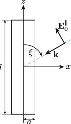
Figure 1: Definition of the geometrical parameters, radius $a$ and length $l$, of the scattering cylinder as well as the chosen body centered coordinate system. Additionally the incident angle $\xi$ and the polarization basis vector $\mathbf{E}_{0}^{\parallel}$ are depicted in the incident plane.

In infinite free space the electric field $\mathbf{E}(\mathbf{r})$ generated by a time harmonic current density distribution $\mathbf{j}(\mathbf{r})$ (time dependence $e^{-i\omega t}$) enclosed in the finite volume $V$ is given by [14]

$$\mathbf{E}(\mathbf{r})=\mathbf{E}^{inc}(\mathbf{r})+i\omega\mu_{0}\left(\overleftrightarrow{\mathbf{I}}+\frac{1}{k^{2}}\nabla\otimes\nabla\right)\\ \int_{V}g(\mathbf{r},\mathbf{r}^{\prime})\mathbf{j}(\mathbf{r}^{\prime})\,d^{3}r^{\prime}$$ (1)

where $\overleftrightarrow{\mathbf{I}}$ denotes the three-dimensional unit tensor, $\otimes$ is the tensor product defined by $\left(\mathbf{a}\otimes\mathbf{b}\right)_{ij}=a_{i}b_{j}$,

$$g(\mathbf{r},\mathbf{r}^{\prime})=\frac{e^{ik\left|\mathbf{r}-\mathbf{r}^{\prime}\right|}}{4\pi\left|\mathbf{r}-\mathbf{r}^{\prime}\right|}$$ (2)

is the scalar Green’s function and $k=\frac{\omega}{c}$ the free space wave number. $\mathbf{E}^{inc}$ is an electric field due to sources not contained in $V$. In scattering problems the driving current density is not controlled from the outside, but instead induced by $\mathbf{E}^{inc}$ which plays the role of an incident field in this case. Spatial derivatives of the integral in (1) exist as long as the source current density $\mathbf{j}(\mathbf{r})$ satisfies the Hölder condition [15], $\left|\mathbf{j}\left(\mathbf{r}\right)-\mathbf{j}(\mathbf{r}^{\prime})\right|\leq k\left|\mathbf{r}-\mathbf{r}^{\prime}\right|^{\alpha}$ with $k>0$ and $0<\alpha\leq 1$ for every pair $\mathbf{r},\mathbf{r}^{\prime}\in V$.

In what follows we consider light scattering on a cylinder (wire) with length $l$ and radius $a$ (Fig. 1). The geometry of the problem including a body centered coordinate system with $z$-axis parallel to the cylinder axis is depicted in figure 1. The wave vector $\mathbf{k}$ enclosing the incident angle $\xi$ with the positive $z$-axis lies in the $xz$-plane (incident plane). To excite longitudinal resonances only the projection of the incident plane wave electric field on the incident plane $\mathbf{E}_{0}^{\parallel}=E_{0}^{\parallel}\left(\sin\xi\hat{\mathbf{z}}-\cos\xi\hat{\mathbf{x}}\right)$ have to be taken into account. The perpendicular polarization component can be safely ignored. Under the assumption that the cylinder diameter is much smaller than the free space wavelength, i.e. $ka\ll 1$, the incident electric field interacting with the cylinder can be viewed as a function depending only on $z$

$$\mathbf{E}^{inc}(z) \approx \mathbf{E}_{0}^{\parallel}e^{-ikz\cos\xi}.$$ (3)

First we briefly review the derivation of Pocklington’s equation for scattering on a thin perfectly conducting wire [1]. In this case in cylindrical coordinates $\left\{\rho,\phi,z\right\}$ the induced current density $\mathbf{j}(\mathbf{r})$ has only a $z$-component, shows no $\phi$-dependence and exists solely on the antenna interface. Then the induced current $I(z)$ is related to the current density $\mathbf{j}(\mathbf{r})$ as

$$\mathbf{j}(\mathbf{r})=\hat{\mathbf{z}}I(z)\frac{\delta(\rho-a)}{2\pi a}$$ (4)

so that

$$I(z)=\int_{0}^{2\pi}d\phi\int_{0}^{a}\rho d\rho\,j(\mathbf{r}).$$ (5)

Using (4) in (1) and performing the $\rho^{\prime}$-integration one yields for the $z$-component of the electric field on the cylinder surface the following integro-differential equation

$$E_{z}(a,z)=E_{z}^{inc}(z)+i\frac{\omega\mu_{0}}{2\pi}\left(1+\frac{1}{k^{2}}\frac{\partial^{2}}{\partial z^{2}}\right)\\ \int_{-\frac{l}{2}}^{\frac{l}{2}}dz^{\prime}\int_{0}^{2\pi}d\phi^{\prime}\,g_{a}(\phi^{\prime},z-z^{\prime})I(z^{\prime}).$$ (6)

where $g_{a}(\phi^{\prime},z-z^{\prime})=g(\mathbf{r},\mathbf{r}^{\prime})$ with $\mathbf{r}=\left(a,0,z\right)$ and $\mathbf{r}^{\prime}=\left(a,\phi^{\prime},z^{\prime}\right)$ in cylindrical coordinates. While the antenna is perfectly conducting, the $z$-component of the total field at the antenna surface has to vanish, $E_{z}(a,z)=0$. Applying this boundary condition to Eq. (6) one can derive Pocklington’s integro-differential equation in the form

$$E_{z}^{inc}(z)=-i\frac{\omega\mu_{0}}{2\pi}\left(1+\frac{1}{k^{2}}\frac{\partial^{2}}{\partial z^{2}}\right)\\ \int_{-\frac{l}{2}}^{\frac{l}{2}}dz^{\prime}\int_{0}^{2\pi}d\phi^{\prime}\,g_{a}(\phi^{\prime},z-z^{\prime})I(z^{\prime}),$$ (7)

which provides a general solution of the scattering problem [1]. Here the fact, that the antenna is perfectly conducting, is taken into account twice, first by assuming a special form of the induced current (4) and second by enforcing the boundary condition $E_{z}(a,z)=0$.

A typical nano-antenna at optical frequency range possesses high, but finite conductivity. In this case the surface current approximation (4) is still applicable, while the boundary condition $E_{z}(a,z)=0$ is generally not. In order to use a Pocklington’s like equation at this frequency range, one needs a relationship between the field $E_{z}(a,z)$ and the current $I(z)$ at the antenna interface.

Assuming a long nanowire, i.e. $l\gg a$, it is reasonable to expect that the internal electric field is separable similar to the solution of the equivalent problem involving an infinite cylinder [10]. Moreover, it can be shown that as long as the wire is electrically thin, i.e. $ka\ll 1$, and $\left|\epsilon_{r}\right|\gg 1$ at least for the case of inclined incidents ($\xi\neq\frac{\pi}{2}$) the $\rho$- and $\phi$-components of the internal field are negligible compared to the $z$-component of the field and the $z$-component shows no $\phi$-dependence. Assuming these conditions are fulfilled the internal electric field can be approximated by

$$\mathbf{E}(\mathbf{r})\approx\hat{\mathbf{z}}f(z)J_{0}\left(k_{\rho}\rho\right)$$ (8)

where $J_{0}\left(k_{\rho}\rho\right)$ denotes the Bessel function of the first kind, $k_{\rho}=k\sqrt{\epsilon_{r}-\cos^{2}\xi}$ with relative permittivity $\epsilon_{r}$ of the wire and $f(z)$ an unknown $z$-dependent function giving the amplitude of the internal field along the wire. A connection between the induced current density and the internal electric field is given by means of the volume equivalence theorem [1] by

$$\mathbf{j}(\mathbf{r})=-i\omega\epsilon_{0}\Delta\epsilon_{r}\mathbf{E}(\mathbf{r})$$ (9)

with $\Delta\epsilon_{r}=\epsilon_{r}-1$. Combining (8) and (9) the total current through the wire can be calculated

$$I(z) =\int_{0}^{2\pi}d\phi\int_{0}^{a}\rho d\rho\,j_{z}(\rho,z)$$

$$=-i\omega\epsilon_{0}\Delta\epsilon_{r}2\pi a\frac{J_{1}\left(k_{\rho}a\right)}{k_{\rho}}f(z).$$ (10)

Further comparing results of the integration in (10) with (8) one can derive the following relation between the electric field and the total current at the wire interface

$$E_{z}(a,z)=Z_{S}I(z)$$ (11)

with the surface impedance

$$Z_{S}=i\frac{J_{0}(k_{\rho}a)k_{\rho}}{2\pi a\omega\epsilon_{0}\Delta\epsilon_{r}J_{1}(k_{\rho}a)}.$$ (12)

Using relation (11) the following Pocklington like integro-differential equation for induced total current, the surface impedance (SI) integro-differential equation [12], can be obtained from equation (6)

$$Z_{S}I(z)=E_{z}^{inc}(z)+i\frac{\omega\mu_{0}}{2\pi}\left(1+\frac{1}{k^{2}}\frac{\partial^{2}}{\partial z^{2}}\right)\\ \int_{-\frac{l}{2}}^{\frac{l}{2}}dz^{\prime}\int_{0}^{2\pi}d\phi^{\prime}\,g_{a}(\phi^{\prime},z-z^{\prime})I(z^{\prime}).$$ (13)

We propose a further improvement to the approximation (13) by releasing the solely surface current ansatz (4). In order to do that, we assume that the induced current density on the right hand side of equation (1) can be factorize similar to the internal field (8). In this way substituting (8) in equation (1) both on the left hand side as boundary condition as well as by using (9) on the right hand side to rewrite the induced current density one obtains a self-consistent integro-differential equation for the unknown amplitude $f(z)$

$$f(z)J_{0}\left(k_{\rho}a\right)=E_{z}^{inc}(z)+k^{2}\Delta\epsilon_{r}\left(1+\frac{1}{k^{2}}\frac{\partial^{2}}{\partial z^{2}}\right)\\ \int_{V}d^{3}r^{\prime}\,g(a,z;\mathbf{r}^{\prime})f(z^{\prime})J_{0}\left(k_{\rho}\rho^{\prime}\right)$$ (14)

where $g(a,z;\mathbf{r}^{\prime})=g(\mathbf{r},\mathbf{r}^{\prime})$ with $\mathbf{r}=\left(a,0,z\right)$ in cylindrical coordinates. This volume current (VC) integro-differential equation takes into account both appropriate boundary conditions at the wire interface and an appropriate volume current distribution inside the wire.

3 Discrete form of VC integral equation

In order to solve numerically the integro-differential equations (13) and (14) one has to impose additional boundary conditions at the nano-antenna edges. A common choice is to impose the total current $I(z)$ to be equal to zero for $z=\pm l/2$ [12]. For a solid wire with finite conductivity this choice is generally not justified, while the total current can be discontinuous at the wire edges [14].

To overcome the requirement of additional boundary condition one has to convert the integro-differential equations into purely integral ones. To do that one has to bring the differential operator $\left(1+k^{-2}\partial_{z}^{2}\right)$ inside the integral. This procedure results in singularities of the order $\left|\mathbf{r}-\mathbf{r}^{\prime}\right|^{3}$ which are generally not integrable over a volume. To treat these singularities we follow the regularization scheme proposed by Lee et al. in Ref. [16]. The regularized VC equation (14) reads:

$$\left(1+\Delta\epsilon_{r}L_{33}\right)E_{z}(a,z)=E_{z}^{inc}(z)+\\ k^{2}\Delta\epsilon_{r}\left\{\int_{V-V^{\star}}G_{33}(a,z;\mathbf{r}^{\prime})E_{z}(\rho^{\prime},z^{\prime})d^{3}r^{\prime}+\right.\\ \int_{V^{\star}}\Biggl{[}G_{33}(a,z;\mathbf{r}^{\prime})E_{z}(\rho^{\prime},z^{\prime})-\\ \frac{1}{k^{2}}\frac{\partial^{2}}{\partial z^{2}}g_{0}(a,z;\mathbf{r}^{\prime})E_{z}(a,z)\Biggr{]}\,d^{3}r^{\prime}\Biggr{\}}$$ (15)

with $E_{z}(\rho,z)=f(z)J_{0}\left(k_{\rho}\rho\right)$. Here $V^{\star}$ denotes a finite and arbitrary shaped principal volume $V^{\star}$ containing the singular point $\mathbf{r}=(a,0,z)$, $g_{0}(\mathbf{r},\mathbf{r}^{\prime})=\lim_{k\rightarrow 0}g(\mathbf{r},\mathbf{r}^{\prime})$ is the static scalar Green’s function, $G_{33}$ is the $zz$-element of the dyadic Green’s function [14]

$$G_{33}(\mathbf{r},\mathbf{r}^{\prime})=\left(1+\frac{1}{k^{2}}\frac{\partial^{2}}{\partial z^{2}}\right)g(\mathbf{r},\mathbf{r}^{\prime}),$$ (16)

and $L_{33}$ the $zz$-element of the source dyadic [14]

$$L_{33}=\frac{1}{4\pi}\oint_{\partial V^{\star}}d^{2}r^{\prime}\,\frac{\left(z^{\prime}-z\right)\left(\hat{\mathbf{n}}\cdot\hat{\mathbf{z}}\right)}{\left|\mathbf{r}-\mathbf{r}^{\prime}\right|^{3}}.$$ (17)

The surface integration in (17) has to be performed over the surface $\partial V^{\star}$ enclosing the principal volume $V^{\star}$, $\hat{\mathbf{n}}$ denotes the outer surface normal.

The main advantage of the regularization scheme [16] is (i) that all singularities disappear and (ii) that the principal volume $V^{\star}$ can be finite and arbitrary shaped. We choose a cylinder with length $\Delta$, radius $\frac{\Delta}{2}$ and center at the singular point $\mathbf{r}=(a,0,z)$ as the principal volume (Fig. 2). We assume $\Delta$ to be small, such that both the Bessel function $J_{0}\left(k_{\rho}\rho^{\prime}\right)$ and the amplitude function $f(z^{\prime})$ are approximately constant over $V^{\star}$. Taking that into account, writing the volume integrals in the regularized VC equation (15) in cylinder coordinates $\left\{\rho,\phi,z\right\}$ and collecting all terms containing $f(z)$ on the left and all terms containing $f(z^{\prime}\neq z)$ on the right hand side, one obtains a one-dimensional integral equation in the form

$$f(z)\Gamma\approx E_{z}^{inc}(z)+\int_{-\frac{l}{2}}^{z-\frac{\Delta}{2}}dz^{\prime}f(z^{\prime})\mathcal{L}(\left|z-z^{\prime}\right|)+\\ \int_{z+\frac{\Delta}{2}}^{\frac{l}{2}}dz^{\prime}f(z^{\prime})\mathcal{L}(\left|z-z^{\prime}\right|),$$ (18)

with

$$\Gamma=J_{0}\left(k_{\rho}a\right)\left\{1+\Delta\epsilon_{r}L_{33}-\eta_{in}\right\}-\eta_{out},$$ (19)

$$\eta_{in}=4k^{2}\Delta\epsilon_{r}\int_{0}^{\frac{\Delta}{2}}d\tilde{z}\\ \left\{\left(\int_{\phi_{min}}^{\pi}d\tilde{\phi}\int_{0}^{\frac{\Delta}{2}}\tilde{\rho}d\tilde{\rho}+\int_{\frac{\pi}{2}}^{\phi_{min}}d\tilde{\phi}\int_{0}^{\rho_{max}\left(\tilde{\phi}\right)}\tilde{\rho}d\tilde{\rho}\right)\right.\\ \left.\left(G_{33}(\mathbf{0},\tilde{\mathbf{r}})-\frac{1}{k^{2}}\frac{\partial^{2}}{\partial z^{2}}g_{0}(\mathbf{0},\tilde{\mathbf{r}})\right)\right\},$$ (20)

$$\eta_{out}=4k^{2}\Delta\epsilon_{r}\int_{0}^{\frac{\Delta}{2}}d\tilde{z}\int_{\phi_{min}}^{\pi}d\tilde{\phi}\int_{\frac{\Delta}{2}}^{\rho_{max}(\tilde{\phi})}\tilde{\rho}d\tilde{\rho}\\ \left\{J_{0}\left[k_{\rho}\rho^{\prime}(\tilde{\rho},\tilde{\phi})\right]G_{33}(\mathbf{0},\tilde{\mathbf{r}})\right\}$$ (21)

and

$$\mathcal{L}(\left|z-z^{\prime}\right|)=2k^{2}\Delta\epsilon_{r}\int_{0}^{a}\rho^{\prime}d\rho^{\prime}J_{0}\left(k_{\rho}\rho^{\prime}\right)\\ \int_{0}^{\pi}d\phi^{\prime}G_{33}(a,z;\rho^{\prime},z^{\prime}).$$ (22)

In (20) the integration is performed over the principal volume $V^{\star}$, while in (21) over the corresponding wire slice of thickness $\Delta$ centered at $z=z^{\prime}$ but with excluded principal volume $V^{\star}$. To calculate these two integrals a new coordinate system with its center at the singular point has been chosen Fig. (2). In the new coordinate system the source dyadic (17) can be explicitly written as

$$L_{33}=\frac{(\pi-\phi_{min})\left(2-\sqrt{2}\right)}{2\pi}+\frac{\left(\phi_{min}-\frac{\pi}{2}\right)}{\pi}-\\ \frac{\Delta}{\pi}\int_{\frac{\pi}{2}}^{\phi_{min}}d\tilde{\phi}\frac{1}{\sqrt{4\rho_{max}^{2}(\tilde{\phi})+\Delta^{2}}}.$$ (23)

The radius vector $\rho^{\prime}$ and the integration ranges in (20,21,23) parametrically depend on the nanowire radius $a$ and the wire slice thickness $\Delta$ and are given by

$$\rho^{\prime}(\tilde{\rho},\tilde{\phi})=\left|\left(\begin{array}[]{c}a\\ 0\end{array}\right)+\left(\begin{array}[]{c}\tilde{\rho}\cos\tilde{\phi}\\ \tilde{\rho}\sin\tilde{\phi}\end{array}\right)\right|,$$ (24)

$$\rho_{max}(\tilde{\phi}) =-2a\cos\tilde{\phi}$$

$$\phi_{min} =\arccos\left[-\frac{\Delta}{4a}\right].$$ (25)

Taking into account that the nanowire diameter is small in comparison to the wavelength one can further simplify the integrals in (20) and (21) by expanding the Green’s function $G_{33}$ in power of $k$ up to the linear term

$$G_{33}^{NF}(R)\approx\frac{1}{4\pi}\left(\frac{3R_{z}^{2}-R^{2}}{k^{2}R^{5}}+\frac{R_{z}^{2}+R^{2}}{2R^{3}}+i\frac{2}{3}k\right)$$ (26)

where $\mathbf{R}=\mathbf{r}^{\prime}-\mathbf{r}$. Using (26) one can analytically integrate equation (20) over $\tilde{z}$ and $\tilde{\rho}$ and equation (21) over $\tilde{z}$ . Residual integration in (20), (21) and (23) has to be performed numerically. The regularization scheme (15) ensures, that numerical integration converges. In this way $\Gamma$ in (18) can be efficiently calculated once for given radius $a$ of the nanowire antenna, $\Delta$ and wavelength.

Equation (18) can be solved numerically by a method of moments (MoM) approach. Specifically we choose a point matching MoM scheme with pulse-function basis [17]. That means we divide the nanowire into a set of slices with thickness $\Delta$ and label each slice with an index $i$. For reasonable thin slices the amplitude function $f(z)$ on each of them can be approximated by its value at the center $f(z_{i})=\mathbf{f}_{i}$. This leads to the $n=\frac{l}{\Delta}$ dimensional matrix equation as discretized version of (18)

$$\left(\Gamma\overleftrightarrow{\mathbf{I}}-\overleftrightarrow{\mathbf{M}}\right)\mathbf{f}=\mathbf{E}^{inc}$$ (27)

where $\mathbf{E}_{i}^{inc}=E_{z}^{inc}(z_{i})$ and

$$M_{ij}=\begin{cases}\int_{z_{j}-\frac{\Delta}{2}}^{z_{j}+\frac{\Delta}{2}}dz^{\prime}\mathcal{L}\left(\left|z_{i}-z^{\prime}\right|\right)&\text{for }i\neq j\\ 0&\text{for }i=j\end{cases}$$ (28)

which can be easily inverted numerically to yield the discrete set of values $f(z_{i})$. While the Green’s function depends on the distance between two slices $\left|z-z^{\prime}\right|$, only the first row $M_{1j}$ of the matrix $M$ has to be calculated. All other elements can be filled using the rule $M_{ij}=M_{i-1,j-1}$.

Using the Green’s function expansion (26) in the calculation of the matrix elements $M_{1j}$ for $j<\frac{2a}{\Delta}$ the integration over $z^{\prime}$ can be done analytically. Only the integration over the nanowire profile has to be done numerically. In the calculation of the matrix elements $M_{1j}$ for $j>\frac{2a}{\Delta}$ the full dyadic Green’s function have to be used and so the complete volume integral has to be done numerically. These integrations are done over $\mathbf{r}^{\prime}$-regions far from the singularity and they demonstrate good convergence. An additional performance improvement can be achieved by expanding the Bessel function $J_{0}$ for small arguments as [18]

$$J_{0}(x)\approx 1-\frac{x^{2}}{4}+\frac{x^{4}}{64}+\mathcal{O}(x^{6}).$$ (29)

Having the amplitude function $f(z)$ calculated from (27) the $z$-component of the induced electric field is given by the ansatz (8).

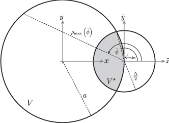
Figure 2: Cross-section of the nanowire (big circle) and the principal volume $V^{\star}$ (small circle) together with the definition of the coordinate systems used to calculate integrals in equation (18).

4 Discrete form of SI integral equation

To solve the surface impedance integro-differential equation (13) the regularization and discretization scheme presented in section 3 can be also applied. A principal volume is chosen as a full slice of the wire at position $z$ with thickness $\Delta$. Regularizing the SI equation (13), writing it in cylinder coordinates and collecting all terms containing $I(z)$ and $I(z^{\prime}\neq z)$, one obtains a one-dimensional integral equation in the form

$$I(z)\Gamma^{S}\approx E_{z}^{inc}+\int_{-\frac{l}{2}}^{z-\frac{\Delta}{2}}dz^{\prime}I(z^{\prime})\mathcal{L}^{S}(\left|z-z^{\prime}\right|)+\\ \int_{z+\frac{\Delta}{2}}^{\frac{l}{2}}dz^{\prime}I(z^{\prime})\mathcal{L}^{S}(\left|z-z^{\prime}\right|)$$ (30)

with

$$\mathcal{L}^{S}(\left|z-z^{\prime}\right|)=i\frac{\omega\mu_{0}}{\pi}\int_{0}^{\pi}d\phi^{\prime}\,G_{33}^{a}(\phi^{\prime},z-z^{\prime})$$ (31)

and

$$\Gamma^{S}=Z_{S}+i\frac{\omega\mu_{0}}{2\pi}\left\{\frac{1}{k^{2}}L_{33}^{S}-4\int_{0}^{\frac{\Delta}{2}}dz^{\prime}\int_{0}^{\pi}d\phi^{\prime}\right.\\ \left.\left[G_{33}^{a}(\phi^{\prime},z^{\prime})-\frac{1}{k^{2}}\frac{\partial^{2}}{\partial z^{2}}g_{0}^{a}(\phi^{\prime},z^{\prime})\right]\right\},$$ (32)

where

$$L_{33}^{S}=\frac{\Delta}{4\pi}\int_{0}^{2\pi}d\phi^{\prime}\,\frac{1}{\sqrt{\left(\frac{\Delta}{2}\right)^{2}+4a^{2}\sin^{2}\left(\frac{\phi^{\prime}}{2}\right)}^{3}}$$ (33)

and $G_{33}^{a}(\phi^{\prime},z-z^{\prime})=G_{33}(\mathbf{r},\mathbf{r}^{\prime})$ as well as $g_{0}^{a}(\phi^{\prime},z-z^{\prime})=\lim_{k\rightarrow 0}g(\mathbf{r},\mathbf{r}^{\prime})$ with $\mathbf{r}=\left\{a,0,z\right\}$ and $\mathbf{r}^{\prime}=\left\{a,\phi^{\prime},z^{\prime}\right\}$ in cylinder coordinates. The source dyadic $L_{33}^{S}$ can be expressed in terms of the complete elliptic integral of the second kind $E\left(m\right)$ [18] as

$$L_{33}^{S}=\frac{1}{\pi}\frac{8}{16a^{2}+\Delta^{2}}E\left(-\frac{16a^{2}}{\Delta^{2}}\right),$$ (34)

where $E\left(m\right)$ is defined by

$$E\left(m\right)=\int_{0}^{\frac{\pi}{2}}\sqrt{1-m\sin^{2}\theta}\,d\theta.$$ (35)

In $\Gamma^{S}$ (32) the $z^{\prime}$-integrations can be performed analytically with the help of the near-field expansion of the Green’s function (26). The residual $\phi^{\prime}$-integration has to be done numerically once for given nanowire radius $a$, $\Delta$ and wavelength.

To solve (30) numerically we use a point matching MoM scheme with pulse function basis [17] as in section 3. Again the nanowire should be divided into a set of slices of thickness $\Delta$ yielding the matrix equation

$$\left(\Gamma^{S}\overleftrightarrow{\mathbf{I}}-\overleftrightarrow{\mathbf{M}}^{S}\right)\mathbf{I}=\mathbf{E}^{inc}$$ (36)

where

$$M_{ij}^{S}=\begin{cases}\int_{z_{j}-\frac{\Delta}{2}}^{z_{j}+\frac{\Delta}{2}}dz^{\prime}\mathcal{L}^{S}\left(\left|z_{i}-z^{\prime}\right|\right)&\text{for }i\neq j\\ 0&\text{for }i=j\end{cases}$$ (37)

and $I_{i}=I(z_{i})$. Similar to the case of volume current integral equation considered in section 3 only the first row of the matrix $\overleftrightarrow{\mathbf{M}}^{S}$ have to be calculated due to the symmetry of the Green’s function. Further for slices with $\left|z_{1}-z_{j}\right|\leq 2a$ the near field approximation of the Green’s function (26) can be used to perform the $z^{\prime}$-integrations in (37) analytically. The remaining integrations as well as the matrix inversion have to be performed numerically. Good convergence of the integrals is ensured, while the integrand is evaluated far from the singular point. Numerical inversion of (36) results in the current $I_{i}=I(z_{i})$ at the discrete number of points $z_{i}$ along the nanowire. Finally the $z$-component of the induced electric field is given via (11).

5 Numerical results and discussion

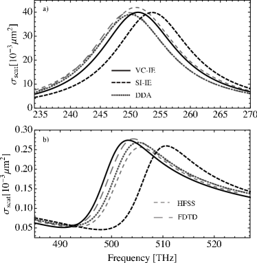
Figure 3: Scattering cross-section of a gold nanowire ($l=200nm,\,a=10nm$) under slanting incidence ($\xi=\frac{\pi}{4}$) calculated with different rigorous numerical methods as well as the proposed volume current and surface impedance one-dimensional integral equations. In the top panel (a) the first and in the bottom panel (b) the third resonance peak are shown.

In this section the semi-analytical methods developed in sections 3 and 4 are evaluated and compared with numerically rigorous methods. Plane wave scattering on a gold nanowire is considered in the optical and near-infrared spectral range. The relative permittivity of gold in this spectral range can be modeled by a free electron Drude model

$$\epsilon_{r}(\omega)\approx\epsilon_{\infty}-\frac{\omega_{p}^{2}}{\omega^{2}+i\gamma\omega}$$ (38)

with parameters $\epsilon_{\infty}=9$, $\omega_{p}=1.36674\cdot 10^{16}\,s^{-1}$ and $\gamma=7.59297\cdot 10^{13}\,s^{-1}$[9]. For comparison purposes we calculate the total scattering cross-section

$$\sigma_{scat}=\frac{\oint_{S}d^{2}r\,\left|\mathbf{E}_{s}\right|^{2}}{\left|\mathbf{E}^{inc}\right|^{2}}$$ (39)

where the scattered electric field $\mathbf{E}_{s}$ is generated by the induced current density $\mathbf{j}(\mathbf{r})$ given by equation (9) in the case of the VC and by equation (4) in the case of the SI integral equation model, respectively. In the far-field zone the scattering field is purely transverse and one can use the far-field dyadic Green’s function

$$\lim_{r\rightarrow\infty}\overleftrightarrow{\mathbf{G}}(\mathbf{r},\mathbf{r}^{\prime})=\frac{e^{ik\left(r-\hat{\mathbf{r}}\cdot\mathbf{r}^{\prime}\right)}}{4\pi r}\left\{\overleftrightarrow{\mathbf{I}}-\hat{\mathbf{r}}\otimes\hat{\mathbf{r}}\right\}$$ (40)

and integral relation

$$\mathbf{E}_{s}(\mathbf{r})=i\omega\mu_{0}\int_{V}d^{3}r^{\prime}\,\overleftrightarrow{\mathbf{G}}(\mathbf{r},\mathbf{r}^{\prime})\mathbf{j}(\mathbf{r}^{\prime})$$ (41)

to calculate the scattering cross-section. For the VC integral equation model the scattering cross section can be written in terms of the amplitude function $f(z)$

$$\sigma_{scat}=\frac{k^{4}a^{4}\pi}{8\left|\mathbf{E}^{inc}\right|^{2}}\left|\Delta\epsilon_{r}\left(1-\frac{1}{8}a^{2}k^{2}\epsilon_{r}\right)\right|^{2}\\ \int_{0}^{\pi}d\theta\,\sin^{3}\theta\left|\int_{-\frac{l}{2}}^{\frac{l}{2}}dz^{\prime}f(z^{\prime})e^{-ik\cos\theta z^{\prime}}\right|^{2}$$ (42)

while for SI integral equation model in terms of the total current $I(z)$

$$\sigma_{scat}^{S}=\frac{\omega^{2}\mu_{0}^{2}}{8\pi\left|\mathbf{E}^{inc}\right|^{2}}\\ \int_{0}^{\pi}d\theta\,\sin^{3}\theta\left|\int_{-\frac{l}{2}}^{\frac{l}{2}}dz^{\prime}I(z^{\prime})e^{-ik\cos\theta z^{\prime}}\right|^{2}.$$ (43)

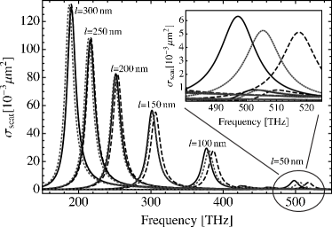
Figure 4: Scattering cross-sections of gold nanowire with fixed radius $a=10nm$ and different lengths. The full and dashed lines show the VC and SI integral equation results, respectively. The dotted line is the numerically rigorous reference calculated using DDA method.

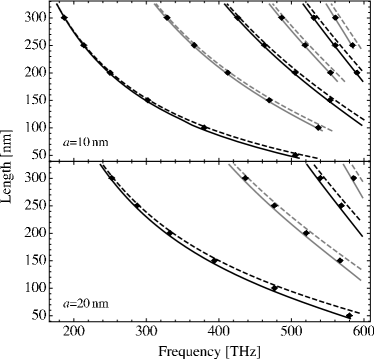
Figure 5: Contours plot of the resonance frequencies of the nanowires with different lengths under slanting incidence ($\xi=\frac{\pi}{4}$). Top panel radius is $a=10nm$, bottom panel $a=20nm$. The full and dashed lines show the VC and SI integral equation results, respectively. The dots are represents the numerically rigorous DDA calculations.

We have performed a systematic convergence test of the developed one-dimensional integral equation based methods for gold nanowires of different lengths and radii. Spatial resolution of $\Delta=1nm$ (thickness of the individual slices in the wire discretization) typically results in less than 1THz discrepancy with respect to the converged value of the scattering cross-section maximum calculated at resolution as small as $\Delta=0.05nm$. In what follows spatial resolution of $\Delta=1nm$ has been used for all calculations based of the VC and SI integral equation models.

In figure 3 the first (top panel) and the third (bottom panel) resonance peaks of the cross-section spectra are shown for a gold nanowire ($a=10nm,\,l=200nm$) under slanting incidence ($\xi=\frac{\pi}{4}$) with $\left|\mathbf{E}^{inc}\right|=1$. Results of both different rigorous numerical methods and semi-analytical 1D ones are compared. For the rigorous numerical calculations we used (i) HFSS, a commercial finite-element frequency-domain Maxwell solver from ANSYS [19], (ii) an in-house implementation of the finite difference time domain method (FDTD) [20] and (iii) ADDA, an open-source software package for calculating scattering parameters using the discrete dipole approximation (DDA) algorithm [21]. The space discretization in the shown DDA and FDTD calculations was set to $1nm$. Discrepancies among the scattering cross-section spectra calculated using different rigorous three-dimensional (3D) Maxwell solvers are comparable with discrepancies of these spectra with the spectrum calculated using VC integral equation method. The accuracy of the SI integral equation method is slightly worse but still very reasonable.

Most important are the differences in used computational resources and execution time. The calculation of one frequency point in VC (SI) integral equation method requires approximately 2 (1) seconds on one core of a workstation using Mathematica [22]. In contrast DDA calculations requires around 8 minutes per frequency point on the same workstation. HFSS needs around 6 minutes per frequency point if the mesh is optimized for one frequency only and is reused without optimization for 30 other frequencies. With FDTD one gets the complete spectra in one run in around 250 minutes on one core. In conclusion the newly proposed 1D semi-analytical methods provide a speed-up in execution time close to 200 times compared to general 3D Maxwell solvers. Additionally up to 100 times less RAM is required for the semi-analytical calculations.

In figure 4 the position of the scattering cross-section maxima are shown for gold nanowires with different aspect ratios. Radius is $a=10nm$ and length varies from $l=50nm$ (shown in the inset) to $l=300nm$. Normal incidence ($\xi=\frac{\pi}{2}$) with $\left|\mathbf{E}^{inc}\right|=1$ is considered. VC integral equation method (full black line), SI integral equation method (dashed line) and DDA (dotted line) are compared. As it is expected the accuracy of both semi-analytical methods deteriorates with decreasing aspect ratio. However even for considerable low aspect ratio $\frac{5}{4}$ ($l=50nm$) the first resonance peak predicted using approximate methods represents the rigorous numerical result with a good relative accuracy (2% of the central frequency).

In general VC integral equation method demonstrate better agreement with the DDA calculations in comparison with the SI method (Fig. 3 and 5). This can be best seen in figure 5, where the resonance frequencies of increasing order (from left to right) against the wire length are depicted for nanowires with radius $a=10nm$ (top panel) and $a=20nm$ (bottom panel). The VC integral equation method (solid line), SI integral equation method (dashed line) are presented. Dots represent DDA results. The brighter (darker) curves are the resonances of even (odd) orders. All calculations are done under slanting incidence ($\xi=\frac{\pi}{4}$). The better accuracy of the VC integral equation method can be systematical traced in figure 5 especially for the structures with smaller aspect ratio.

6 Conclusion

Two alternative methods to solve the scattering problem on optical nanowire antenna, the volume current integral equation (VC-IE) method and the surface impedance integral equation (SI-IE) method are introduced. In order to reduce the general 3D volume integral equation describing the scattering problem to a simple semi-analytical 1D integro-differential equation, both methods utilize solutions of the problem of plane wave scattering on infinite cylinder. A regularization and discretization scheme is proposed in order to transform integro-differential equations into solely integral equation. This transformation enables to solve the original problem without necessity to impose additional boundary conditions at the nanowire edges. Numerical evaluation of the proposed methods and their comparison with different numerically rigorous methods is presented for scattering cross-section calculations. Gold nanowires are analyzed at optical and near-infrared spectral range. The introduced one-dimensional semi-analytical methods demonstrate good agreement and superior numerical performance in comparison with rigorous numerical methods.

References

• [1] C.ย A. Balanis, Advanced engineering electromagnetics, Wiley, 1989.
• [2] J.ย Volakis, Antenna Engineering Handbook, Fourth Edition, McGraw-Hill Professional, 2007.
• [3] P.ย Bharadwaj, B.ย Deutsch, L.ย Novotny, Optical Antennas, Advances in Optics and Photonics 1ย (3) (2009) 438.
• [4] P.ย Mรผhlschlegel, H.-J. Eisler, O.ย J.ย F. Martin, B.ย Hecht, D.ย W. Pohl, Resonant optical antennas., Science (New York, N.Y.) 308ย (5728) (2005) 1607โ€“9.
• [5] L.ย Rogobete, F.ย Kaminski, M.ย Agio, V.ย Sandoghdar, Design of plasmonic nanoantennae for enhancing spontaneous emission, Optics Letters 32ย (12) (2007) 1623.
• [6] T.ย H. Taminiau, F.ย D. Stefani, F.ย B. Segerink, N.ย F. van Hulst, Optical antennas direct single-molecule emission, Nature Photonics 2ย (4) (2008) 234โ€“237. doi:10.1038/nphoton.2008.32.
• [7] G.ย Raschke, S.ย Kowarik, T.ย Franzl, C.ย Sรถnnichsen, T.ย A. Klar, J.ย Feldmann, A.ย Nichtl, K.ย Kรผrzinger, Biomolecular Recognition Based on Single Gold Nanoparticle Light Scattering (May 2003).
• [8] H.ย A. Atwater, A.ย Polman, Plasmonics for improved photovoltaic devices., Nature materials 9ย (3) (2010) 205โ€“13.
• [9] V.ย Myroshnychenko, J.ย Rodrรญguez-Fernรกndez, I.ย Pastoriza-Santos, A.ย M. Funston, C.ย Novo, P.ย Mulvaney, L.ย M. Liz-Marzรกn, F.ย J. Garcรญa De Abajo, Modelling the optical response of gold nanoparticles., Chemical Society reviews 37ย (9) (2008) 1792โ€“805.
• [10] C.ย F. Bohren, D.ย R. Huffman, Absorption and Scattering of Light by Small Particles, Wiley-VCH, 1998.
• [11] B.ย P. Sinha, R.ย H. MacPhie, Electromagnetic scattering by prolate spheroids for plane waves with arbitrary polarization and angle of incidence, Radio Science 12ย (2) (1977) 171โ€“184.
• [12] G.ย W. Hanson, On the Applicability of the Surface Impedance Integral Equation for Optical and Near Infrared Copper Dipole Antennas, IEEE Transactions on Antennas and Propagation 54ย (12) (2006) 3677โ€“3685.
• [13] M.ย Yurkin, A.ย Hoekstra, The discrete dipole approximation: An overview and recent developments, Journal of Quantitative Spectroscopy and Radiative Transfer 106ย (1-3) (2007) 558โ€“589.
• [14] J.ย Bladel, Electromagnetic fields, Wiley-IEEE, 2007.
• [15] O.ย D. Kellogg, Foundations of potential theory, Courier Dover Publications, 1953.
• [16] S.ย W. Lee, J.ย Boersma, C.ย L. Law, G.ย Deschamps, Singularity in Greenโ€™s function and its numerical evaluation, Antennas and Propagation, IEEE Transactions on 28ย (3) (1980) 311โ€“317.
• [17] S.ย J. Orfanidis, Electromagnetic Waves and Antennas, http://www.ece.rutgers.edu/~orfanidi/ewa/, 2010.
• [18] I.ย A. Stegun, M.ย Abramowitz, Handbook of Mathematical Functions: with Formulas, Graphs, and Mathematical Tables, Dover Publications, 1965.
• [19] Ansys hfss, http://www.ansoft.com/products/hf/hfss/.
• [20] A.ย Taflove, S.ย C. Hagnes, Computational Electrodynamics: The Finite-Difference Time-Domain Method, Artech House, 2000.
• [21] M.ย Yurkin, V.ย Maltsev, A.ย Hoekstra, The discrete dipole approximation for simulation of light scattering by particles much larger than the wavelength, Journal of Quantitative Spectroscopy and Radiative Transfer 106ย (1-3) (2007) 546โ€“557.
• [22] Wolfram mathematica 8, http://www.wolfram.com/mathematica.