Bubble statistics and positioning in superhelically stressed DNA

Abstract

We present a general framework to study the thermodynamic denaturation of double-stranded DNA under superhelical stress. We report calculations of position- and size-dependent opening probabilities for bubbles along the sequence. Our results are obtained from transfer-matrix solutions of the Zimm-Bragg model for unconstrained DNA and of a self-consistent linearization of the Benham model for superhelical DNA. The numerical efficiency of our method allows for the analysis of entire genomes and of random sequences of corresponding length ($10^{6}–10^{9}$ base pairs). We show that, at physiological conditions, opening in superhelical DNA is strongly cooperative with average bubble sizes of $10^{2}–10^{3}$ base pairs (bp), and orders of magnitude higher than in unconstrained DNA. In heterogeneous sequences, the average degree of base-pair opening is self-averaging, while bubble localization and statistics are dominated by sequence disorder. Compared to random sequences with identical GC-content, genomic DNA has a significantly increased probability to open large bubbles under superhelical stress. These bubbles are frequently located directly upstream of transcription start sites.

I Introduction

Fundamental processes, such as transcription and replication require a transient, local opening of the DNA double helix calladine ; alberts . Such bubbles occur spontaneously under physiological conditions kowalski88 ; kowalski89 , while complete melting and the separation of the two complementary strands requires temperatures around $80^{o}$C FK . Bubbles have been implicated as an explanation for high cyclization rates in short DNA fragments cloutier ; yan , but their main interest lies in biology and in the physical mechanism underlying the functioning and control of transcription and replication start sites: the stability of DNA is sequence-dependent SL and opening is strongly influenced by superhelical stress benham92 ; fye99 ; benham06 and the binding of regulatory proteins sobellPNAS85 ; ambjornsson05 . In particular, Benham and coworkers showed significant correlations between the positions of strongly stress-induced destabilized regions and regulatory sites wang04 ; ak05 ; wang08 .
Several models exist to describe the internal opening of DNA. The Peyrard-Bishop-Dauxois peyrard89 ; dauxois93 and the Poland-Scheraga (PS) models poland ; jostBJ09 have already been used to quantify bubble statistics kalosakas04 ; vanerp05 ; ares07 ; kafri02 ; blossey03 ; garel05 ; coluzzi07 ; monthus07 and for the ab initio annotation of genomes on the basis of correlations between biological function and thermal melting yeramian02 ; carlon07 ; jostJPCM09 . Here, we describe the bubble statistics of random and biological sequences at physiological conditions using (i) the Zimm-Bragg (ZB) model, an efficient approximation of the PS model jostJPCM09 , and (ii) the Benham model fye99 , a generalization of the ZB model accounting for superhelical density but neglecting writhe. After exploring the bubble statistics of unconstrained DNA using the ZB model, we introduce an asymptotically exact self-consistent linearization vologodskii of the Benham model as a precise and convenient tool to study the huge impact of superhelicity on local bubble opening. The numerical efficiency of the method allows us to investigate the bubble statistics for entire genomes and random sequences of sufficient length ($10^{6}-10^{9}$ bp) to obtain statistically significant results for sequence effects on bubble statistics and positioning. In a final step, we correlate the positions of highly probable bubbles within the genome of E. coli with the position of transcription start sites (TSS) and start codons.

II Models and Methods

II.1 Unconstrained DNA

II.1.1 The Zimm-Bragg model

The most widely-used model to treat the denaturation of DNA chains is the PS model poland which offers predictive power for thermal melting and strand dissociation for DNA of arbitrary length, strand concentration and a wide range of ionic conditions. For long heterogeneous sequences, whose local denaturation is dominated by the quenched sequence disorder garel05 ; coluzzi07 ; monthus07 , the related and computationally faster ZB model gives surprisingly good results jostJPCM09 . In the PS and ZB formalisms, the free energy of a given configuration is decomposed into formation free energies for closed base-pair steps and free energy penalties for the nucleation of unpaired regions (or bubbles). Using periodic boundary conditions, the ZB Hamiltonian for a circular chain of length $N$ can be expressed as jostJPCM09

$$\mathcal{H}_{ZB}=\sum_{i=1}^{N}\left\{(\Delta g_{i}-\Delta g_{loop})\theta_{i}\theta_{i+1}+\Delta g_{loop}\theta_{i}\right\}$$ (1)

where $\theta_{i}=0$ ($1$) if base-pair $i$ is open (closed). $\Delta g_{i}$ ($\sim k_{b}T$) is the nearest-neighbor (NN) free energy to form the base-pair step $(i,i+1)$. $\Delta g_{loop}\equiv-k_{B}T\log[\sigma_{PS}\bar{L}^{-c}]$ is the loop nucleation penalty and depends on the PS cooperativity $\sigma_{PS}\sim 10^{-4}$, on the interacting self-avoiding loop exponent $c\sim 2.1$ kafri02 ; blossey03 and on a typical bubble length $\bar{L}$ jostJPCM09 ($\Delta g_{loop}\sim 20k_{b}T$ for $\bar{L}=170$). Parameters are taken at physiological conditions for temperature $T=37^{o}$ C and salt concentration $[Na^{+}]=0.1$ M jostJPCM09 .

II.1.2 Transfer-matrix method

Being formulated as a 1D Ising model, the model is easily solved analytically (numerically) for homogeneous (heterogeneous) sequences using transfer matrix methods. The partition function of the system is then given by jostJPCM09

$$\mathcal{Z}=\textrm{Trace}\left[\prod_{i=1}^{N}T_{i}\right],$$ (2)

the individual closing probability by

$$\langle\theta_{i}\rangle=\frac{1}{\mathcal{Z}}\textrm{Trace}\left[\left(\prod_{j=1}^{i-1}T_{j}\right)T^{\prime}_{i},\left(\prod_{j=i+1}^{N}T_{j}\right)\right].$$ (3)

In particular, it is possible to calculate position resolved opening probabilities, $P_{i,l}$, for bubbles containing $l$ open bps and beginning at the closed bp $i$, by

$$P_{i,l}=\frac{1}{\mathcal{Z}}\textrm{Trace}\left[\left(\prod_{j=1}^{i-1}T_{j}\right)T^{\prime}_{i}ST^{\prime}_{i+l+1}\left(\prod_{j=i+l+2}^{N}T_{j}\right)\right]$$ (4)

with

$$T_{i}=\left(\begin{array}[]{cc}e^{-\beta\Delta g_{i}}&e^{-\beta\Delta g_{loop}}\\ 1&1\end{array}\right),$$

$$T^{\prime}_{i}=\left(\begin{array}[]{cc}e^{-\beta\Delta g_{i}}&e^{-\beta\Delta g_{loop}}\\ 0&0\end{array}\right)\quad\textrm{and}\quad S=\left(\begin{array}[]{cc}0&0\\ 1&1\end{array}\right).$$

The global closing probability $\Theta$ and the probability per bp $P_{l}$ to observe a bubble of length $l$ are given by $\Theta=(\sum_{i=1}^{N}\langle\theta_{i}\rangle)/N$ and $P_{l}=(\sum_{i=1}^{N}P_{i,l})/N$. Basic summing rules on the bubble probabilities imply that $1-\Theta=\sum_{l}lP_{l}$, and that $\mathcal{L}=(\sum_{l}lP_{l})/(\sum P_{l})=(1-\Theta)/P_{b}$,

$$\mathcal{L}=\frac{\sum_{l}lP_{l}}{\sum P_{l}}=\frac{1-\Theta}{P_{b}}$$ (5)

where $\mathcal{L}$ is the average bubble length and $P_{b}=\sum_{l}P_{l}$ is the probability per bp to observe a bubble of arbitrary length.

For homogeneous sequences, these equations could be solved easily. In the asymptotic limit $N\rightarrow\infty$, it leads to

$$\mathcal{Z} = \left[\frac{1+g+\sqrt{(g-1)+4s}}{2}\right]^{N},$$ (6)

$$\langle\theta\rangle = \frac{1}{2}\left[1+\frac{g-1}{\sqrt{(g-1)^{2}+4s}}\right],$$ (7)

$$P_{l} = \frac{1}{2}\left[\frac{2}{1+g+\sqrt{(g-1)^{2}+4s}}\right]^{l+2}$$ (8)

$$\times\left[\frac{2s+g\left(g-1+\sqrt{(g-1)^{2}+4s}\right)}{\sqrt{(g-1)^{2}+4s}}\right]$$

with $g=\exp[-\beta\Delta g]$ and $s=\exp[-\beta\Delta g_{loop}]$. The bubble probability is therefore a decreasing exponential function of $l$ for homogeneous sequences.

For heterogeneous sequences, we numerically compute the different desired observables in a $\mathcal{O}(N)$-algorithm. In a first step, we iteratively compute the forward and backward products, $F_{i}=\left(\prod_{j=1}^{i}T_{j}\right)$ and $B_{i}=\left(\prod_{j=i}^{N}T_{j}\right)$. The second step consists in applying equations 2, 3 and 4.

II.2 Superhelical DNA

In living organisms, DNA is highly topologically constrained into circular domains (closed-loops or circular molecules) calladine . Each closed domain is defined by a topological invariant $L$, the so-called linking number. $L$ represents the algebraic number of turns either strand of the DNA makes around the other. It can be decomposed in two contributions: the twist which is the number of turns of the double-helix around its central axis, and the writhe which is the number of coils of the double-helix. In the majority of living systems, the average linking number $L$ is below the characteristic linking number value $L_{o}$ of the corresponding unconstrained linear DNA, due to a negative superhelical density $\sigma=\alpha A/N\approx-0.06$ imposed by protein machineries, where $\alpha=L-L_{o}$ is the linking number difference.

II.2.1 The Benham model

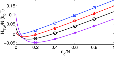
Figure 1: Effective superhelical hamiltonian $\mathcal{H}_{TW}$ per bp as a function of the relative opening $n_{o}/N$ in the asymptotic limit, for different stress values: $\sigma=0$ (squares), -0.03 (stars), -0.06 (circles) and -0.1 (crosses).

In this article, we consider bubble openings in superhelically constrained circular DNA using the Benham model for an imposed superhelical density $\sigma$, where the standard thermodynamic description of base-pairing ($\mathcal{H}_{ZB}$) is coupled with torsional stress energetics benham92 ; fye99 . For each state, if one neglects the writhe contribution, the imposed linking difference $\alpha$ can be decomposed in three contributions: 1) the denaturation of $n_{o}$ base-pairs relaxes the helicity by $-n_{o}/A$ where $A=10.4$ bp/turn is the number of base-pair in a helical turn; 2) the resulting single-strand regions can twist around each other inducing a global over-twist of $\mathcal{T}$; 3) then, the bending and twisting of double-stranded parts is put in the residual linking number $\alpha_{r}$. Therefore, due to the topological invariance of $\alpha$, we get the closure relation

$$\alpha=-\frac{n_{o}}{A}+\mathcal{T}+\alpha_{r}$$ (9)

For denatured regions, the high flexibility of single-stranded DNA allows unpaired strands to interwind. The energy associated with the helical twist $\tau_{i}$ (in rad/bp) of open base-pair $i$ is

$$\mathcal{H}_{tw}(\theta_{i},\tau_{i})=\frac{C}{2}(1-\theta_{i})\tau_{i}^{2}$$ (10)

where the torsional stiffness $C$ is known from experiments, $C\approx 3.09k_{B}T$. The individual twist $\tau_{i}$ are related to the global over-twist $\mathcal{T}$ via the relation $\mathcal{T}=\sum_{i}(1-\theta_{i})\tau_{i}/(2\pi)$. For paired helical regions, it has been experimentally found that superhelical deformations induce an elastic energy, quadratic in the residual linking difference

$$\mathcal{H}_{r}=\frac{K}{2}\alpha_{r}^{2}=\frac{K}{2}\left(\alpha+\frac{n_{o}}{A}-\mathcal{T}\right)^{2}$$ (11)

where $n_{o}=\sum_{i}(1-\theta_{i})$ is the number of open base-pairs and $K\equiv K^{\prime}/N\approx 2220k_{B}T/N$. By integrating over the $n_{o}$ continuous degrees of freedom $\tau_{i}$, the superhelical stress energetics is represented by a non-linear effective Hamiltonian fye99 :

$$\mathcal{H}_{TW}(n_{o}) = \frac{2\pi^{2}CK}{4\pi^{2}C+Kn_{o}}\left[\alpha+\frac{n_{o}}{A}\right]^{2}$$ (12)

$$-\frac{1}{2\beta}\log\left(\left[\frac{2\pi}{\beta C}\right]^{n_{o}}\frac{4\pi^{2}C}{4\pi^{2}C+Kn_{o}}\right)$$

$\mathcal{H}_{TW}$ is minimal for a non-zero number of opening base-pairs which increases as the stress strength increases (see figure 1).
The total effective Hamiltonian is given by $\mathcal{H}_{eff}(\{\theta_{i}\})=\mathcal{H}_{ZB}(\{\theta_{i}\})+\mathcal{H}_{TW}(n_{o})$. We fix $\Delta g_{loop}=20k_{b}T$.

II.2.2 Torque-imposed ensemble

The Benham Hamiltonian is defined in a superhelical density ($\sigma$)-imposed ensemble defined by equation 9. In this section, we briefly discuss similar model but in the torque-imposed ensemble.
In this ensemble, a linear DNA segment (length $N$) is constraint by a weak torque $\Gamma$ applied on base $N$, the first bp being fixed. For each bp $i$, we define $\omega_{i}$ its orientation in the plane perpendicular to the average axis of the double-helix and oriented in the 5’ to 3’ direction (for a denatured bp-step, $\delta\omega_{i}\equiv\omega_{i+1}-\omega_{i}=\tau_{i}/(2\pi)$ of the Benham model). The total Hamiltonian of the system is then given by orland

$$\mathcal{H} = H_{ZB}+\frac{C}{2}\sum_{i}(1-\theta_{i})(\delta\omega_{i})^{2}$$ (13)

$$+\frac{K_{r}}{2}\sum_{i}\theta_{i}(\delta\omega_{i}-\omega_{0})^{2}-\Gamma(\omega_{N}-\omega_{1})$$

with $K_{r}=K^{\prime}/(4\pi^{2})$ and $\omega_{0}=2\pi/A$ the natural helical twist. Writing $(\omega_{N}-\omega_{1})=\sum_{i}\delta\omega_{i}$, and integrating over the $\delta\omega_{i}$, leads to the effective Hamiltonian (relatively to the situation without torque):

$$\mathcal{H}_{eff}=\mathcal{H}_{ZB}+\left[\Gamma^{2}\left(\frac{1}{2C}-\frac{1}{2K_{r}}\right)-\Gamma\omega_{0}\right]\sum_{i}\theta_{i}$$ (14)

Applying the constant torque $\Gamma$ is therefore equivalent to adding an external field $h_{e}=-[\Gamma^{2}(1/(2C)-1/(2K_{r}))-\Gamma\omega_{0}]$ in the ZB formalism.

II.3 Self-consistent linearization

II.3.1 Solving the Benham model

Recently, Jeon et al jeonPRL10 derived formulas to solve the Benham model for homogeneous and random heterogeneous sequences, including the computation of sequence-average bubble properties. The computation is based on a reorganization of the partition function sum into partial sums for fixed numbers of bubbles.

For heterogeneous sequences, Fye and Benham fye99 proposed an exact $\mathcal{O}(N^{2})$-algorithm by decomposing the prefactor $\exp[-\beta\mathcal{H}_{TW}(n_{o})]$ in discrete Fourier modes, and by using the transfer-matrix method. Benham and coworkers benham04 ; bi03 ; bi04 have also developed an approximate method which first involves a windowing procedure to find the minimum free energy and then consider only the states whose energies do not exceed the minimum one by more than a given threshold. At high threshold values or high negative superhelicity, the computation time for this algorithm scales exponentially with the threshold and the superhelical stress. Both schemes are still time demanding for very long sequences.

II.3.2 Self-consistent field

In order to speed up the resolution of the Benham model and to access directly to position-dependent opening properties of bps and bubbles, we develop an efficient variational method vologodskii allowing us to use the transfer-matrix solution of the ZB model. For long sequences, assuming that fluctuations of $n_{o}$ are small around the value $\bar{n}_{o}$, we can expand $\mathcal{H}_{TW}(n_{o})$ around $\bar{n}_{o}$. The approximated effective Hamiltonian then takes the typical ZB form:

$$\mathcal{H}_{eff}\approx\mathcal{H}_{ZB}(\{\theta_{i}\})+\mathcal{H}_{TW}(\bar{n}_{o})+(N-\bar{n}_{o})h-h\sum_{i=1}^{N}\theta_{i}$$ (15)

where $h=(\partial\mathcal{H}_{TW}/\partial n_{o})(\bar{n}_{o})$ represents the mean-field of our approximation. If one imposes the superhelical stress $\Gamma$ (ie, the torque) instead of the superhelical density, $h$ is related to the effective field $(4\pi^{2}N/K-1/C)(\Gamma^{2}/2)+2\pi\Gamma/A$ generated by the torque (see above).
In the following, we employ the Benham ensemble of an imposed superhelical density, $\sigma$, and determine $h$ (or $\Gamma$) self-consistently. Self-consistency requires $\langle n_{o}\rangle(\bar{n}_{o})=\bar{n}_{o}$, and is equivalent to solving

$$h=(\partial\mathcal{H}_{TW}/\partial n_{o})(\langle n_{o}\rangle(h)),$$ (16)

because the function $(\partial\mathcal{H}_{TW}/\partial n_{o})(n_{o})$ is monotonic.

II.3.3 Homogeneous sequences

For homogeneous sequences, the general solution of the self-consistency equation 16 cannot be computed analytically. However, at low temperatures, weak superhelical densities and in the limit of infinitely long chains, a small perturbation development is valid and leads to analytical expressions for $h$. For infinitely long chains, $\mathcal{H}_{TW}$ becomes

$$\mathcal{H}_{TW}(x)/N=\frac{2CK^{\prime}\pi^{2}(\sigma+x)^{2}}{A^{2}(4C\pi^{2}+K^{\prime}x)}-f\,x$$ (17)

with $x=n_{o}/N$, $K^{\prime}=NK$ and $f=-\log[2\pi/(\beta C)]/(2\beta)$. Assuming that the fraction of open base-pairs $x$ is small ($x<<1$), $\partial\mathcal{H}_{TW}/\partial n_{o}=\partial(\mathcal{H}_{TW}/N)/\partial x$ is given by

$$\left(-f+\frac{K^{\prime}\sigma}{A^{2}}-\frac{K^{\prime 2}\sigma^{2}}{8A^{2}C\pi^{2}}\right)+K^{\prime}\left(\frac{[K^{\prime}\sigma-4\pi^{2}C]^{2}}{A^{2}(4\pi^{2}C)^{2}}\right)x+o(x^{2})$$ (18)

Using Eq.7 and noting $y=\exp[\beta h]$, we also have

$$x\approx\frac{sy}{(gy-1)^{2}}$$ (19)

In the limit $gy>>1$, inserting $x\approx s/(g^{2}y)$ in Eq.18 and solving Eq.16, leads to

$$h^{*}=-f+\frac{K^{\prime}\sigma(8C\pi^{2}-K^{\prime}\sigma)}{8A^{2}C\pi^{2}}$$ (20)

This expression is valid until $gy\sim 1$ ($h\approx\Delta g$), i.e.

$$\sigma\approx\left(\frac{2\pi}{K^{\prime}}\right)\left(2\pi C-\sqrt{2C(2\pi^{2}C-A^{2}[f-\Delta g])}\right)\equiv\sigma_{l}$$ (21)

For $\sigma<\sigma_{l}$, we could write $gy=1+\epsilon$ (with $\epsilon>0$). Then, $x\approx(s/g)/\epsilon^{2}$ and $h\approx\Delta g+\epsilon$. Solution of Eq.16 leads to

$$h^{*}=\Delta g+\left(\sqrt{\frac{K^{\prime}s}{2\pi^{2}Cg}}\right)(4C\pi^{2}-K^{\prime}\sigma)\left(\frac{4C\pi^{2}-K^{\prime}\sigma}{\sqrt{8A^{2}\pi^{2}fC+K^{\prime}\sigma(K^{\prime}\sigma-8\pi^{2}C)+8A^{2}\pi^{2}C\Delta g}}\right)$$ (22)

Figure 2 shows that the numerical solution of Eq.16 agrees very well with the two expressions found above (Eq.20 and 22).

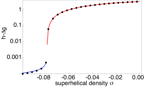
Figure 2: Numerical (dots) or analytical (lines) solutions of the self-consistency equation Eq.16 for a homogeneous sequence ($\Delta g=-3.14k_{B}T$).

To compute bp or bubbles properties, formulas 6, 7 and 8 are still available if one replaces $g$ by $g\,y$ and $s$ by $s\,y$.

II.3.4 Heterogeneous sequences

For heterogeneous sequences, we use the bisection method coupled to the Newton-Raphson method press to numerically solve the self-consistency equation, for fixed values of the temperature and of the superhelical density. Knowing that an evaluation of the function $f$ requires one transfer matrix method computation ($\mathcal{O}(N)$ each), it takes typically $10-20$ evaluations to determine the root with a relative precision of $10^{-4}$. This allows numerically efficient computation of denaturation profiles. For example, computing the local closing probabilities for the E.coli genome ($N\sim 4.6$ Mbps) takes about $70$ seconds on a 2.4 GHz computer with the self-consistent method, whatever the density is. On the same computer, it would take about $10^{10}$ s with the exact method ($\mathcal{O}(N^{2})$ algorithm) for any $\sigma$ values (interpolation of data given in Ref.fye99 ), and about $6.10^{4}$ s with the approximate method for $\sigma=-0.055$ ( and around 40 times more for $\sigma=-0.075$) benham04 ; bi03 ; bi04 .

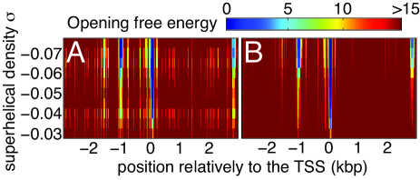
Figure 3: (Color online) Opening free energy $-\log[1-\langle\theta_{i}\rangle]$ for the extended neighborhood of the TSS of Fig. 10, computed using the Benham’s web server benhamweb (A) or using our formalism (B).

II.3.5 Comparison with the Benham model

The self-consistent linearization consists in working in the torque-imposed ensemble and determining the torque self-consistently to better approximate the superhelical density-imposed ensemble. This representation has the advantage of decoupling the opening of different parts of the molecule and is probably the simplest way to express the destabilizing effect of undertwisting on DNA stability. In the thermodynamic limit, i.e., for very long (genomic) sequences and at low temperature (well below the melting temperature), we expect our linearization to be a quasi-exact solution of the Benham model due to the asymptotic decrease of fluctuations within the system. For shorter sequences, however, the non-linearity of the effective superhelical Hamiltonian $\mathcal{H}_{TW}$ (see Eq.12) may significantly couple remote domains along the sequence, leading for example, to the closing of an open domain as one increases the superhelical stress (as observed in Fig.3A). Although, the self-consistent linearization neglects such effects, it gives a reliable general picture of the superhelically-stressed destabilization of DNA sequences. In figure 3, we show a comparison of results obtained from the Benham web server bi04 ; benhamweb and by our method. The agreement is excellent and the small deviations are mostly due to the slightly different parametrizations of the ZB parts and to the absence of finite size effect in our approach as discussed above.

III Results and Discussion

In the following, we discuss results obtained for random homogeneous and heterogeneous sequences, as well as for some bacterial genomes (E.coli, T. whipplei, A. Baumanii, B. subtilis and S. coelicolor, see Table 1). The results shown for random heterogeneous sequences were obtained by compiling profiles from 100 random sequences each containing $10^{6}$ bp.

III.1 Melting of superhelical DNA

The melting properties of constrained DNAs reflect a balance between the two parts of $\mathcal{H}_{eff}$. At $37^{o}$ C, $\mathcal{H}_{ZB}$ opposes local opening the more strongly the higher the GC-content of the sequence. In contrast, $\mathcal{H}_{TW}$ is minimal for a finite number of open base-pairs, which increases as $\sigma$ becomes more negative. At biological levels, the free energy of completely closed DNA becomes prohibitively large (see Fig.1). As a consequence, superhelicity leads to a notable level of base-pair opening at physiological temperatures, where unconstrained DNA exhibits negligible breathing.

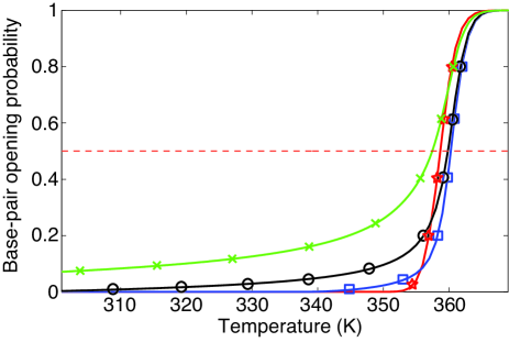
Figure 4: Evolution of the global opening probability $1-\Theta$ as a function of temperature for an unconstrained (stars) or constrained ($\sigma=0$: squares, $\sigma=-0.06$: circles, $\sigma=-0.2$: crosses) random sequence (GC=0.5).

Figure 4 shows the overall impact on the opening probability of imposing a superhelical constraint. For comparison, we have also included a melting curve for unconstrained DNA. At physiological temperatures, the unconstrained DNA is very stable whereas the superhelicity significantly contributes to opening of base pairs and bubbles. However, for intermediate and weak negative stresses, the destabilizing effect of an imposed superhelical density is reversed close to the melting temperature due to the overall stabilizing impact of untwisting on the rest of the DNA ($\mathcal{H}_{TW}(n_{o}=N/2)>0$), resulting in a slowdown of the melting process via a change of $\Gamma$ (or $h$) with temperature. This effect has already been pointed out for positively-stressed homogeneous molecules benham96 . For stronger stresses, the effective twisting Hamiltonian $\mathcal{H}_{TW}$ at the melting transition ($n_{o}=N/2$) is still negative and then results in a decrease of the melting temperature. A quantification on this salt-, GC-dependent effect is described below.

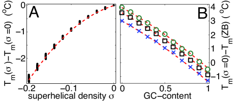
Figure 5: (A) Melting temperature for random sequences (GC$\in[0,1]$) at different salt concentrations ($[Na^{+}]\in[0.05,1]$ M) as a function of the superhelical density $\sigma$ (dots), respectively to the situation with $\sigma=0$. (B) Melting temperature at $\sigma=0$ for random sequences as a function of their GC-content, at $[Na^{+}]=0.05$ (circles), 0.1 (squares) and 0.3 M (crosses), respectively to the corresponding unconstrained (ZB) situation. Dashed lines represent the fitted relation given in Eq.23.

On figure 5 A, we observe that, under the different considered GC-contents and salt concentrations, the melting temperature of random superhelical DNA is a quadratic function of $\sigma$, and only the intercept of this function ($T_{m}(\sigma=0)$) depends on the GC and on $[Na^{+}]$ (see figure 5 B). From a systematic study of the melting temperature $T_{m}$ as a function of the GC-content and the salt concentration, we fitted the empirical relation (in ^o C):

$$\Delta T_{m}([Na^{+}],\textrm{GC},\sigma) = 2.35-0.54\log[Na^{+}]-3.42\textrm{GC}$$ (23)

$$-0.93\textrm{GC}^{2}+4.7\sigma-46.8\sigma^{2}$$

where $\Delta T_{m}$ is the difference in melting temperature between a constrained and an unconstrained random DNA polymers.

Figure 6: (Color online) Evolution at $T=37^{o}$ C of the global opening probability $1-\Theta$ for superhelically constrained random heterogeneous (full lines) and homogeneous (dashed lines) DNAs under different $\sigma$ (from -0.02 to -0.1 every 0.01: color scale from light to dark red, $\sigma=-0.06$: blue line) and for several bacterial genomes at $\sigma=-0.06$: E. coli (triangles), T. whipplei (squares), A. Baumanii (diamonds), B. subtilis (circles) and S. coelicolor (stars). Inset: proportion of the different contributions to the linking number difference $\alpha$: relaxation due to denaturation $-n_{o}/N$ (I), over-twist of the denatured regions $\mathcal{T}$ (II) and residual linking number $\alpha_{r}$ (III) (see Eq.9).

Figure 6 shows the dependance of the opening probability $1-\Theta$ as a function of the GC-content. Results are reported for different levels of superhelical density and at $T=37^{o}$ C, in the biological relevant range, i.e the overall degree of opening is small yet strongly increased relative to the unconstrained case (see also Fig.4). We have included results for both homogeneous and heterogeneous systems. In the former case, the employed NN-free energies $\Delta g$ were determined as composition dependent averages over the tabulated step parameters SL ; jostBJ09 .
Passing a threshold jeonPRL10 (see Inset in Fig.6) depending on the GC-content, strong $\sigma$-values allow the opening of many bp along the sequences. For a fixed superhelical stress, as expected, $1-\Theta$ is a decreasing function of the GC-content. Differences between homogeneous and heterogeneous are weak, meaning that sequence heterogeneity self-averages and has only a small effect on the total degree of opening.
The inset in figure 6 shows the different contributions to the linking number difference as a function of the superhelical density (see Eq.9) for random sequences with GC=0.5. The over-twist $\mathcal{T}$ contribution is estimated by integrating over the $n_{o}$ continuous degrees of freedom $\tau_{i}$ fye99 and applying the self-consistent linearization:

$$\langle\mathcal{T}\rangle = \sum_{\{\theta_{i}\}}\frac{Kn_{o}}{4\pi^{2}C+Kn_{o}}(\alpha+n_{o}/A)\frac{e^{-H_{eff}(\{\theta_{i}\})}}{\mathcal{Z}}$$ (24)

$$\approx \frac{K\langle n_{o}\rangle}{4\pi^{2}C+K\langle n_{o}\rangle}(\alpha+\langle n_{o}\rangle/A)$$ (25)

We observe that the over-twist increases linearly with the opening probability. While for weak stresses, almost all the superhelical energy is stored in the (residual) deformations of the double-helix, for strong stresses, more than 50 % of the imposed superhelical constraint is used to drive the local denaturation of bps. Accounting for the writhe in the model should however decrease the contributions due to bp-denaturation and over-twisting since a part of the constraint would be absorbed by coils of the double-helix.

III.2 Sequence heterogeneity and bubble statistics in superhelical DNA

III.2.1 Bubble statistics in unconstrained DNA

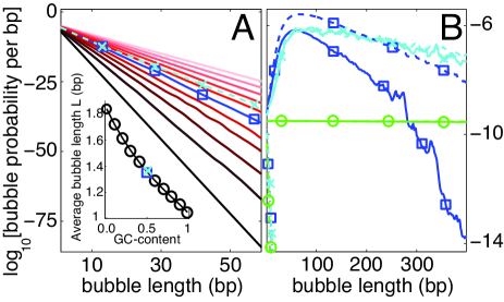
Figure 7: (Color online) Evolution of the bubble probability per bp $P_{l}$ to observe a bubble of length $l$. (A) For unconstrained molecules: random sequences of different GC-content (GC from 0 to 1 every 0.1: color scale from light to dark red, GC=0.5: squares) and the genome of E. coli (dashed line with crosses, GC=0.51). Inset: average bubble length $\mathcal{L}$ as a function of the GC-content. (B) For superhelically-stressed molecules: a random sequence ($GC=0.5$, squares), the genome of E. coli (crosses) and a homogeneous sequence (with $\Delta g=-1.9k_{B}T$ equals to the average NN-free energies in E. coli, circles), and $\sigma=0$ (dotted and dashed lines), $-0.06$ (full lines) and -0.1 (dashed lines).

Figure 7A shows the bubble probabilities computed with the ZB model for random DNAs of different GC-content, with $\Delta g_{loop}=10k_{b}T$ consistent with very small loops ($\bar{L}\sim\mathcal{L}\sim 1$, see inset in Fig.7 A). We remark an exponential decrease of $P_{l}$ with very short decay lengths, corresponding to fairly closed molecules. Increasing GC-content stabilizes the DNA and reduces average bubble lengths. Even accounting for the weak biological sequence effect apparent in our results, the absolute level of bubble opening in unconstrained DNA seems too small for natural breathing to play a direct biological role benham06 .

Whereas we obtain similar $\mathcal{L}$-values as reported for the Peyrard-Bishop-Dauxois (PBD) model ares07 , absolute probabilities $P_{l}$ are far lower (for example $P_{l}\sim 10^{-11}$ (ZB) versus $\sim 10^{-5}$ (PBD) for $l=10$ and GC=0.5), mainly due to the absence of a cooperativity penalty factor preventing bubble formation in the PBD model.

III.2.2 Bubble statistics in superhelical DNA

Figure 7B highlights the huge impact of the superhelical stress on the bubble statistics. For physiological levels, the opening probability per bp remains significant even for large bubbles and has increased by many orders of magnitude compared to the unconstrained situation. For example, for GC=0.5 and $\sigma=-0.06$, $P_{l=10}\approx 10^{-9}$ and $P_{l=60}\approx 10^{-7}$ for superhelical DNA, while for the corresponding unconstrained DNA, we found $P_{l=10}\approx 10^{-11}$ and $P_{l=60}\approx 10^{-41}$.

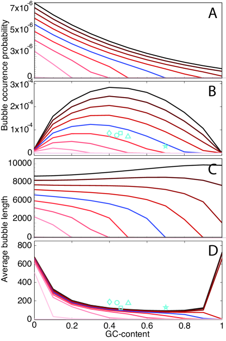
Figure 8: (Color online) Evolution of bubble occurrence probability $P_{b}$ (A,B) and of the average bubble length $\mathcal{L}$ (C,D) for superhelically constrained random heterogeneous (B,D) and homogeneous (A,C) DNAs under different stresses $\sigma$ (from -0.02 to -0.1 every 0.01: color scale from light to dark red, $\sigma=-0.06$: blue line) and for several bacterial genomes at $\sigma=-0.06$: E. coli (triangles), T. whipplei (squares), A. Baumanii (diamonds), B. subtilis (circles) and S. coelicolor (stars).

Figure 8 shows the evolution of the bubble occurence $P_{b}$ and of the average bubble length $\mathcal{L}$ for different $\sigma$-values and GC-content. With $\mathcal{H}_{TW}(n_{0})$ only being a function of the total number of open base-pairs, bubble sizes in homogeneous systems are determined by a competition between the bubble initiation penalty, $\Delta g_{loop}$, favoring the opening of a small number of large bubbles, and entropy, favoring the opening of a large number of small bubbles. In heterogeneous systems, it is possible to lower the fraction of stable GC-steps in the open domains by denaturing a larger number of smaller bubbles in particularly AT-rich regions (see Fig.9) hwa03 . The comparison in Figs. 8 and 9 shows that the disorder effect dominates in the present case garel05 ; coluzzi07 ; monthus07 with the number of bubbles being maximal around GC=0.5. For biological superhelicities, $\mathcal{L}\approx 700$ for random AT- and GC-DNAs, while $\mathcal{L}\approx 150$ for $0.2<f_{GC}<0.9$.

Sequence-heterogeneity plays an essential role by lowering the fraction of stable GC-steps in the open domains and leads to a localization of open base-pairs in (AT-enriched) stress-induced duplex destabilized regions wang04 ; ak05 ; wang08 , whose length in turn limits the bubble sizes. Indeed, figure 9 shows that bubbles appear mainly in AT-enriched regions compared to the background GC-content. Interestingly, for intermediate (biological) $\sigma$ values, the evolution of the GC-composition of bubbles remains flat over a large range of global GC-content.

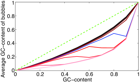
Figure 9: (Color online) Evolution of the average GC-content of bubbles for superhelically constrained random heterogeneous DNAs under different stresses $\sigma$ (from 0 to -0.1 every 0.01: color scale from light to dark red, $\sigma=-0.06$: blue line). The dashed line represents results for homogeneous sequences.

III.3 Bubble statistics in biological DNA

Compared to random sequences with identical GC-content, bacterial genomes (E.coli, T. whipplei, A. Baumanii, B. subtilis and S. coelicolor) exhibit higher averages degrees of opening and increased average bubble sizes (symbols in Figs.6 and 8). Figure 7B shows striking discrepancies in the bubble distribution $P_{l}$ between random and biological sequences, with a significant enrichment of large bubbles. In the latter case, the nearly flat distributions resemble those expected for homogeneous sequences and can be viewed as a signature of large stress-induced destabilized domains, which concentrate the DNA breathing into large regions with homogeneous opening profiles. We also note that the level of opening in the biological domains is comparatively insensitive to the precise level of the superhelical density.

Table 1: Z-scores computed relatively to the average bubble length for 5 prokaryotic organisms.

Organism	$N$ (Mbp)	GC-content	Z-score
A. baumanii	3.98	0.40	23.0
B. subtilis	4.21	0.44	21.0
E. coli	4.64	0.50	25.7
S. coelicolor	8.67	0.70	17.6
T. whipplei	0.93	0.46	10.6

In general, biological sequences are more destabilized than random sequences with a same GC-content, leading to less but longer bubbles. We estimate these differences by computing, for all genomes, the Z-score relatively to $\mathcal{L}$ (see Tab.1). The Z-score is an estimation of the non-randomness of a specific sample. For the average bubble length $\mathcal{L}$, it can be computed by

$$Z=\frac{\mathcal{L}(\mathrm{genome})-\langle\mathcal{L}(\mathrm{random})\rangle}{\sigma_{\mathcal{L}(\mathrm{random})}}$$ (26)

where $\langle\mathcal{L}(\mathrm{random})\rangle$ and $\sigma_{\mathcal{L}(\mathrm{random})}$ are the mean and the standard deviation of $\mathcal{L}$ computed on 100 random sequences with the same GC and length as the corresponding genome. The Z-score represents therefore the distance between a specific point and the mean value obtained for random sequences, given in standard deviation units. Z-scores of 20 for $\mathcal{L}$ suggests the presence of over-represented long AT-rich domains in bacterial genomes which have the ability to easily open under superhelical stress. Interestingly, the organism with the lowest Z-score (T. whipplei) was shown to exhibit a random-like behavior relatively to the local melting temperature distribution jostJPCM09 .

III.4 Bubble positioning in the promoter regions of biological DNA

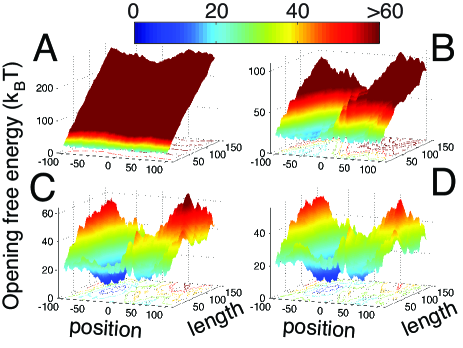
Figure 10: (Color online) Free energies to open a bubble of a given length centered around a given nucleotide ($-k_{B}T\log[P_{i,l}]$) for the neighborhood of a transcription start site (bp n^o 259382) in the E. coli genome, in the presence (B, C, D) or in the absence (A) of an imposed superhelical density $\sigma=-0.03$ (B), -0.06 (C) and -0.10 (D).

Positions of strongly stress-induced destabilized regions have been shown to correlate with many regulatory regions wang08 including transcription start sites wang04 or origins of replication ak05 . In this section, we focus on bubble positioning inside the promoter regions of the bacterium E. coli.
The transcription of DNA is initiated by the local opening of the double-helix at transcription start sites. Figure 3 illustrates their association with strongly stress-induced destabilized regions. In addition to position-dependent opening probabilities, our approach allows us to calculate the complete bubble free-energy landscape, $G_{i,l}=-k_{B}T\log P_{i,l}$. Figure 10 shows the effect of superhelicity on $G_{i,l}$ for the neighborhood of the same TSS in E. coli. The analysis reveals that opening is the result of the meta-stable unwinding of a large bubble and not of enhanced small scale breathing. We note that knowledge of $G_{i,l}$ is essential for modeling the dynamics of bubble nucleation and growth ambjornsson07 .

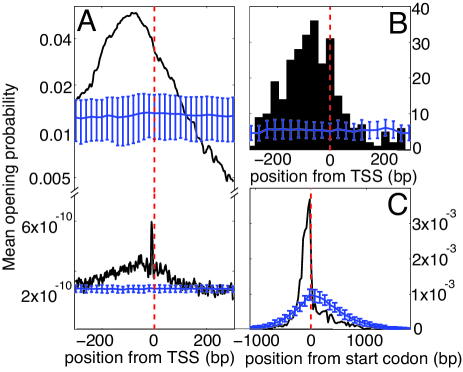
Figure 11: (A) Opening probability as a function of the position relatively to the TSS, averaged on 760 promoter regions of E. coli regulondb (black line), or on 760 randomly picked regions inside the genome (blue line), for a constrained (top) or unconstrained (down) DNA. (B) Histogram of the highly probable ($P_{i,l}\geq 10^{-5}$) bubble centers included in the regions [TSS-300,TSS+300] for the 760 studied TSS (black bars) or for randomly picked regions (blue line). (C) Probability distribution function of the distance between highly probable bubble centers and the nearest start codons for the 1158 actually found (black line) or randomly situated (blue line) bubbles.

Figure 11 analyses the statistical relation beween TSSs and bubbles induced by superhelical stress for the entire genome of E. coli. Figure 11A shows a significant and non-random destabilization around TSSs, with a maximal opening around $-80$. The same computation using the ZB model shows insignificant and orders-of-magnitude smaller opening probabilities. However, we find a non-random signal around TSS-10 corresponding to the position of the AT-rich Pribnow box, an essential motif to start transcription in bacteria pribnowPNAS75 . Figure 11B gives the relative positions of highly probable bubbles included in TSS neighborhoods. The centers of these bubbles are mainly localized in the [TSS-200,TSS] region where many transcriptional and promoter factors are recruited and bind to DNA regulondb . Conversely, figure 11C confirms that the majority of highly probable bubbles are situated upstream and close to start codons of genes. Actually, these bubbles are composed by around $36\%$ of coding bps, significantly lower than the percentage of coding bps in E. coli ($88\%$).

IV Summary and Conclusion

We have developed a numerically efficient, self-consistent solution of the Benham model of bubble opening in superhelically constrained DNA. In particular, we are able to go beyond the calculation of opening probabilities for base pairs and to address the full, position-dependent bubble statistics for entire genomes. Our results indicate, that negative supercoiling leads to (meta-) stable unwinding of bubbles comprising ${\cal O}(100-1000)$ base-pairs. In heterogeneous sequences, bubbles are strongly localized in AT-rich domains with sequence disorder dominating the bubble statistics. As we have shown, large bubbles open with a significantly larger probability in biological sequences, than in random sequences with identical GC-content. In the case of E. coli, the most likely bubbles are located directly upstream from transcription start sites, highlighting the biological importance of this now well understood, physical property of DNA.

References

- (1) C. Calladine, H. Drew, B. Luisi, and A. Travers, Understanding DNA; the molecule and how it works (Elsevier Academic Press, 2004).
- (2) B. Alberts, D. Bray, J. Lewis, M. Raff, K. Roberts, and J.D. Watson, Molecular biology of the cell (Garland Science, 2002).
- (3) D. Kowalski, and M. Eddy, Proc. Natl. Acad. Sci. USA 85, 9464 (1988).
- (4) D. Kowalski, D. Natale, and M. Eddy, EMBO J. 8, 4335 (1989).
- (5) M. Frank-Kamenetskii, Biopolymers 10, 2623 (1971).
- (6) T.E. Cloutier, and J. Widom, Mol. Cell 14, 355 (2004).
- (7) J. Yan, and J.F. Marko, Phys. Rev. Lett. 93, 108108 (2004).
- (8) J. SantaLucia, Proc. Natl. Acad. Sci. USA 95, 1460 (1998).
- (9) C.J. Benham, J. Mol. Biol. 225, 835 (1992).
- (10) R.M. Fye, and C.J. Benham, Phys. Rev. E 59, 3408 (1999).
- (11) C.J. Benham, and R.R.P. Singh, Phys. Rev. Lett. 97, 059801 (2006).
- (12) H.M. Sobell, Proc. Natl. Acad. Sci. USA 82, 5328 (1985).
- (13) T. Ambjörnsson, and R. Metzler, Phys. Rev .E 72, 030901 (2005).
- (14) H. Wang, M. Noordewier, and C.J. Benham, Genome Res. 14, 1575 (2004).
- (15) P. Ak, and C.J. Benham, PLoS Comp. Biol. 1, e7 (2005).
- (16) H. Wang, and C.J. Benham, PLoS Comp. Biol. 4, e17 (2008).
- (17) M. Peyrard, and A.R. Bishop, Phys. Rev. Lett. 62, 2755 (1989).
- (18) T. Dauxois, M. Peyrard, and A.R. Bishop, Phys. Rev. E 47, R44 (1993).
- (19) D. Poland, and H.A. Scheraga, J. Chem. Phys. 47, 1456 (1966).
- (20) D. Jost, and R. Everaers, Biophys. J. 96, 1056 (2009).
- (21) G. Kalosakas, K.O. Rasmussen, A.R. Bishop, C.H. Choi, and A. Usheva, Europhys. Lett. 68, 127 (2004).
- (22) T.S. van Erp, S. Cuesta-Lopez, J.-G. Hagmann, and M. Peyrard, Phys. Rev. Lett. 95, 218104 (2005).
- (23) S. Ares, and G. Kalosakas, Nano Lett. 7, 307 (2007).
- (24) Y. Kafri, D. Mukamel, and L. Peliti, Eur. J. Phys. B 27, 135 (2002).
- (25) R. Blossey, and E. Carlon, Phys. Rev. E 68, 061911 (2003).
- (26) T. Garel and C. Monthus, J. Stat. Mech., P06004 (2005).
- (27) B. Coluzzi, and E. Yeramian, Eur. J. Phys. B 56, 349 (2007).
- (28) C. Monthus, and T. Garel, arXiv:cond-mat/0605448v1 (2007).
- (29) E. Yeramian, S. Bonnefoy, and G. Langsley, Bioinformatics 18, 1 (2002).
- (30) E. Carlon, A. Dkhissi, M.L. Malki, and R. Blossey, Phys. Rev. E 76, 051916 (2007).
- (31) D. Jost, and R. Everaers, J. Phys.: Condens. Matter 21, 034108 (2009).
- (32) A.V. Vologodskii, A.V. Lukashin, V.V., Anshelevich, and M. Frank-Kamenetskii, Nucleic Acids Res. 6, 967 (1979).
- (33) T. Garel, H. Orland, and E. Yeramian, arXiv:q-bio.BM/0407036 (2004).
- (34) C.J. Benham, and C. Bi, J. Comput. Biol. 11, 519 (2004).
- (35) C. Bi, and C.J. Benham, Proceedings of the 2003 IEEE Bioinformatics Conference, (IEEE Computer Society, 2003).
- (36) W.H. Press, S.A. Teukolsky, W.T. Vetterling, and B.P. Flannery, Numerical recipes in FORTRAN: the art of scientific programming (Cambridge University Press, 1992).
- (37) C. Bi and C.J. Benham, Bioinformatics 20, 1477 (2004).
-
(38)
Benham’s web-server:
http://benham.genomecenter.ucdavis.edu. - (39) J.-H. Jeon, J. Adamcik, G. Dietler, and R. Metzler, Phys. Rev. Lett. 105, 208101 (2010).
- (40) C.J. Benham, Phys. Rev. E 53, 2984 (1996).
- (41) T. Hwa, E. Marinari, K. Sneppen, and L.-h. Tand, Proc. Natl. Acad. Sci. USA 100, 4411 (2003).
- (42) T. Ambjörnsson, S.K. Banik, O. Krichevsky, and R. Metzler, Biophys. J. 92, 2674 (2007).
- (43) S. Gama-Castro et al, Nucleic Acids Res. 36, D120 (2008).
- (44) Pribnow, D., Proc. Natl. Acad. Sci. USA 72, 784 (1975).