Light-induced current in molecular junctions: Local field and non-Markov effects

Abstract

We consider a two-level system coupled to contacts as a model for charge pump under external laser pulse. The model represents a charge-transfer molecule in a junction, and is a generalization of previously published results [B. D. Fainberg, M. Jouravlev, and A. Nitzan. Phys. Rev. B 76, 245329 (2007)]. Effects of local field for realistic junction geometry and non-Markov response of the molecule are taken into account within finite-difference time-domain (FDTD) and on-the-contour equation-of-motion (EOM) formulations, respectively. Our numerical simulations are compared to previously published results.

I Introduction

Driven transport and coherent control at the nanoscale are well established areas of research. Quantum ratchets,Hänggi (2011); Roeling et al. (2011) molecular charge,Siegle et al. (2010) spinHanson et al. (2007); Bogani and Wernsdorfer (2008) and heat pumps,Nitzan (2007); Wang et al. (2007) and nano-plasmonicsHalas (2010) are just several examples of areas of recent developments. Advances in optical techniques, in particular near-field optical microscopy, allow single molecule manipulationHildner et al. (2011) and induction of bond specific chemistry.Gordon et al. (1999) Combined with molecular junction fabrication techniques,Ward et al. (2007) optical spectroscopy methods are becoming an important observation and diagnostic tool in molecular electronics.Ward et al. (2008); Ioffe et al. (2008); Ward et al. (2011)

Experimental developments led to surge of theoretical activity in the field of optically assisted transportKohler et al. (2004); Galperin et al. (2006); Viljas et al. (2007, 2008) and optical response of molecular junctions.Galperin and Nitzan (2005, 2006); Harbola et al. (2006); Galperin and Tretiak (2008); Sukharev and Galperin (2010); Galperin et al. (2009a, b)

In particular, Ref. Galperin et al., 2006 considered molecular junctions composed of molecules with strong charge-transfer transition into their excited statePonder and Mathies (1983); Colvin and Alivisatos (1992); Smirnov and Braun (1998) as a possible constituent for light-induced molecular charge pump, when change of molecular dipole occurs along the junction axis. Consideration was done within a two-level (HOMO-LUMO) model with ground and excited (HOMO and LUMO) states of the molecule strongly coupled to different contacts. In junction setup optical excitation brings electron from occupied ground to empty excited state, and asymmetry in coupling to contacts assures appearance of current. The model was treated within non-equilibrium Green function approach, and perturbation theory in coupling to laser field was employed.

Later Ref. Fainberg et al., 2007 generalized the consideration of Ref. Galperin et al., 2006 to strong laser fields. Pumping optical field was treated as a classical driving force, and closed set of EOMs for observables (electronic populations and coherences of the levels and single time exciton correlation function) was formulated. One of the most important advances in Ref. Fainberg et al., 2007 was consideration of chirped laser pulses, which allowed formulation of charge transfer between ground and excited states in terms of Landau-Zener problem. Chirped laser pulses enable to produce complete population inversion in molecular systems (a molecular bridge) where the well-known $\pi$-pulse excitationAllen and Eberly (1975) fails.

In realistic molecular junctions optical field driving the molecule is a local field formed by both incident radiation and scattered response of the system (mostly plasmonic response of metallic contacts). Another feature of molecular junctions is hybridization of states of a molecule with those of contacts. The latter leads to non-Markov effects in response of the junction.

In this paper we generalize studies reported in Ref. Fainberg et al., 2007 incorporating the aforementioned effects into consideration. Dynamics of local electromagnetic fields is simulated within the FDTD technique for realistic geometry of a molecular junction similar to our previous publication.Sukharev and Galperin (2010) Non-Markov effects of junction response are introduced within non-equilibrium Green functions equation-of-motion (NEGF-EOM) approach.

Structure of the paper is the following. After introducing the model in section II, we describe a junction geometry and numerical approach used in calculations of local electromagnetic fields in section III. Section IV discusses calculation of local field-induced electron flux through the junction, and section V introduces set of NEGF-EOMs. Numerical results and discussion are given in section VI. Section VII summarizes our findings.

II Model

A model junction consists of a molecule coupled to two metallic contacts driven by external radiation field. The radiation is a time-dependent local electromagnetic field $E(t)$ calculated within FDTD technique for bowtie geometry of the contacts (see section III for details). Molecule is represented by a two-level system $|1>$ and $|2>$ (HOMO and LUMO or ground and excited states), and is placed in a ‘hot spot’ of the local field. Contacts $L$ and $R$ are assumed to be free charge carrier reservoirs, each at its own equilibrium. Difference in their electrochemical potentials defines bias applied to the junction $eV=\mu_{L}-\mu_{R}$. Following Refs. Galperin et al., 2006; Fainberg et al., 2007 we consider two types of coupling between molecule and contacts: charge and energy transfer. Hamiltonian of the junction is

$$\hat{H}(t)= \hat{H}_{0}(t)+\hat{V}$$ (1)

$$\hat{H}_{0}(t)= \sum_{m=1,2}\varepsilon_{m}\hat{n}_{m}+\sum_{k\in\{L,R\}}\varepsilon_{k}\hat{n}_{k}$$ (2)

$$- \mu E(t)\left(\hat{D}_{12}+\hat{D}_{12}^{\dagger}\right)$$

$$\hat{V}= \sum_{m=1,2}\sum_{k\in\{L,R\}}\left(V_{km}\hat{c}_{k}^{\dagger}\hat{d}_{m}+\mbox{H.c.}\right)$$

$$+ \sum_{k_{1}\neq k_{2}\in\{L,R\}}\left(V^{en}_{k_{1}k_{2}}\hat{c}_{k_{1}}^{\dagger}\hat{c}_{k_{2}}\hat{D}_{12}+\mbox{H.c.}\right)$$ (3)

Here $\hat{d}_{m}^{\dagger}$ ($\hat{d}_{m}$) and $\hat{c}_{k}^{\dagger}$ ($\hat{c}_{k}$) are creation (annihilation) operators of electron in level $m$ of the molecule and in state $k$ in the contact(s), respectively, $\hat{n}_{m}=\hat{d}_{m}^{\dagger}\hat{d}_{m}$ is the operator of electronic population in level $m$, $\hat{D}_{12}\equiv\hat{d}_{1}^{\dagger}\hat{d}_{2}$ is operator of molecular de-excitation ($\hat{D}_{21}\equiv\hat{D}_{12}^{\dagger}$), and $\mu$ is molecular transition dipole moment. Terms on the right-hand side of (2) represent molecular structure (two-level system), contacts, and coupling to the driving field. Right-hand side of Eq.(II) introduces electron and energy transfer between molecule and contact(s). Eqs. (1)-(II) introduce the model of Ref. Fainberg et al., 2007 with rotating wave approximation relaxed, and with driving force treated as a local electromagnetic field.

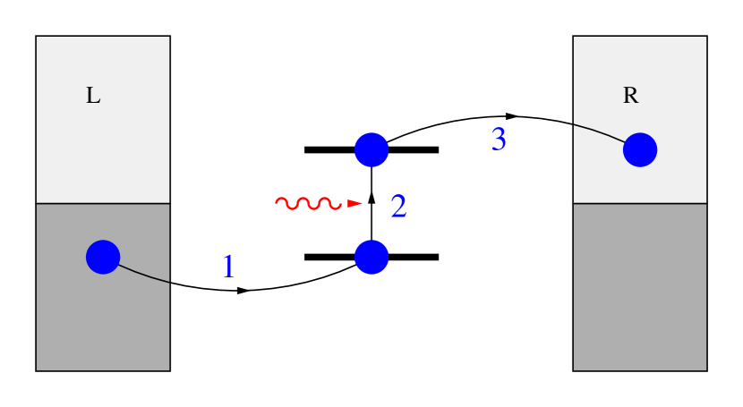
Figure 1: (Color online) A sketch of local field driven molecular charge pump.

To simulate molecules with strong charge-transfer transition with dipole moment oriented along the junction axis below we assume that ground state (or HOMO), $|1>$, is coupled strongly to the left contact $L$, while excited state (or LUMO) - to the right contact $R$. Such setup works as a local field driven charge pump (see Fig. 1). Note that similar selective coupling can also be obtained for the bridge made of a quantum dots as discussed in Refs. Bryllert et al., 2002; Sanchez et al., 2008; Li et al., 2010.

III Local field simulations

Calculations of the local electromagnetic field dynamics are carried out utilizing FDTD technique.Taflove and Hagness (2005) Following Ref. Fainberg et al., 2007 we assume that the incident field, $E_{\mbox{inc}}(t)$, has the form of a linear chirped pulse

$$E_{\mbox{inc}}(t)=\mbox{Re}\left(\mathcal{E}_{0}\exp\left(-\frac{\left(\delta^{2}-i\bar{\mu}\right)t^{2}}{2}-i\omega_{0}t\right)\right),$$ (4)

where $\mathcal{E}_{0}$ is the incident peak amplitude, $\omega_{0}$ is the incident frequency, and parameters $\delta$ and $\bar{\mu}$ describing incident chirped pulse are given by

$$\delta^{2}= \frac{2\tau_{0}^{2}}{\tau_{0}^{4}+4\Phi^{\prime\prime}{}^{2}(\omega_{0})},$$ (5)

$$\bar{\mu}= -\frac{4\Phi^{\prime\prime}(\omega_{0})}{\tau_{0}^{4}+4\Phi^{\prime\prime}{}^{2}(\omega_{0})},$$ (6)

with $\tau_{0}\equiv t_{p0}/\sqrt{2\log{2}}$ (the value of the pulse duration $t_{p0}$ of the corresponding transform-limited pulse used in simulations is $9.34$ fs) and $\Phi^{\prime\prime}(\omega_{0})$ is the chirp rate in the frequency domain. Throughout the simulations the incident field is taken in the form of (4) and is normalized to preserve the total energy of a laser pulse at different chirp rates according to

$$\int_{-\infty}^{+\infty}dtE_{inc}^{2}(t)=\mbox{const}.$$ (7)

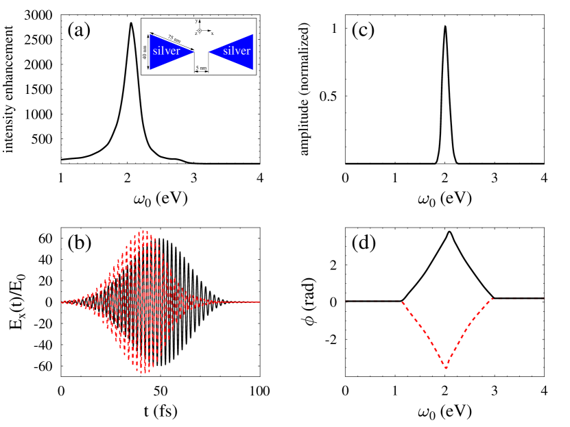
Figure 2: (Color online) Results of FDTD simulations for chirped pulses exciting the bowtie antenna schematically depicted in the inset of panel (a). Panel (a) shows the enhancement of the local intensity $\left|\vec{E}\right|^{2}$ detected in the gap of the bowtie antenna as a function of the incident frequency. Panel (b) presents local field component of electric field along the axis of symmetry of the structure, $E_{x}$, as a function of time for two chirp rates at the plasmon resonance, $\omega_{0}=2.057$ eV: black solid line - $\Phi^{\prime\prime}(\nu_{0})=-3000$ fs², red dashed line - $\Phi^{\prime\prime}(\nu_{0})=3000$ fs². Panel (c) shows the amplitude of the local field in the frequency domain (note that it is independent from the phase rate). Panel (d) represents the phase of the local field in the frequency domain at two chirped rates: black solid line - $\Phi^{\prime\prime}(\nu_{0})=-3000$ fs², red dashed line - $\Phi^{\prime\prime}(\nu_{0})=3000$ fs².

The geometry considered is depicted in the inset of Fig. 2a showing the top view of the bowtie antenna. To investigate the influence of chirped incident pulses on plasmon dynamics we choose incident field in the form (4) and vary $\Phi^{\prime\prime}(\nu_{0})=4\pi^{2}\Phi^{\prime\prime}(\omega_{0})$. Below we shall write $\Phi^{\prime\prime}$, having in mind $\Phi^{\prime\prime}(\nu_{0})$. We further presume that the incident pulse is $x$-polarized and propagates along the $z$ axis with the incident frequency at the plasmon resonance (see the inset of Fig. 2a). Material dispersion of silver is taken in the Drude form with other numerical parameters as in Ref. Sukharev and Galperin, 2010. For a given set of material and geometric parameters the local electric field enhancement exhibits well pronounced plasmon resonance as seen in Fig. 2a reaching the value of 2800 near $2$ eV.

Our goal is to take plasmonic effects (local field enhancement and phase accumulation) directly into account and investigate how such crafted local fields affect transport properties of molecular junctions placed in the gap of bowtie antennas. However it is informative first to examine general features of chirped pulses interacting with plasmonic materials. It has been noted in several papers Stockman et al. (2004); Lee and Gray (2005); Aeschlimann et al. (2007); Cao et al. (2010) that local field enhancement depends sensitively on the sign of chirped excitation pulses. Moreover careful examination of spatiotemporal dependence of local fields on chirp ratesCao et al. (2010) revealed a complex dynamics of plasmon wavepackets that are noticeably influenced by chirped laser pulses - one may find different local points for a given plasmonic system, where positive chirps lead to higher local fields and the other way around.

Generally speaking, plasmonic materials can be considered as pulse shapers Weiner (2009) due to high material dispersion near plasmon resonance, which induces a phase in the frequency domain resulting in shaping of the total electromagnetic field in time domain. This is illustrated in Fig. 2b-d, where one can clearly see that the positive chirp leads to the compression of the local field (Fig. 2b) and hence stronger field enhancement. While the field amplitude in the frequency domain is not affected by the chirp sign (Fig. 2c), obviously the phase of the field is significantly different for positive and negative chirp as shown in Fig. 2d. We note that one can not recover data obtained for negative chirp, for instance, by simply flipping the sign of the phase for the positive chirp. Additional phase induced by the plasmonic system, which depends on the sign of the chirp rate, makes this problem time irreversible.Stockman et al. (2004)

IV Current through the junction

Time-dependent current through the junction under external driving isJauho et al. (1994); Sukharev and Galperin (2010)

$$I_{K}(t)= -\frac{e}{\hbar}\left(\mbox{Tr}\left[\mathbf{\Gamma}^{K}\,\mathbf{\rho}(t)\right]\right.$$ (8)

$$+ \left.\frac{1}{\pi}\mbox{Im}\int_{-\infty}^{+\infty}dE\,f_{K}(E)\,\mbox{Tr}\left[\mathbf{\Gamma}^{K}\,\mathbf{G}^{r}(t,E)\right]\right)$$

Here the trace is taken over molecular subspace, $\mathbf{\Gamma}^{K}$ is matrix of electronic decoherence due to coupling to contact K

$$\Gamma^{K}_{mm^{\prime}}\equiv 2\pi\sum_{k\in K}V_{mk}\,V_{km^{\prime}}\,\delta(E-\varepsilon_{k})$$ (9)

which is energy independent in the wide-band approximation, $f_{K}(E)$ is Fermi-Dirac thermal distribution in the contacts, $\mathbf{\rho}(t)\equiv-i\mathbf{G}^{<}(t,t)$ is non-equilibrium reduced density matrix of molecular subsystem, $\mathbf{G}^{r,<}(t,t^{\prime})$ are matrices in molecular subspace of retarded and lesser projections of single-electron Green function

$$G_{mm^{\prime}}(\tau,\tau^{\prime})\equiv-i\langle T_{c}\,\hat{d}_{m}(\tau)\,\hat{d}_{m^{\prime}}^{\dagger}(\tau^{\prime})\rangle$$ (10)

($T_{c}$ is contour ordering operator), and $\mathbf{G}^{r}(t,E)$ is the right side Fourier transform of the retarded Green function

$$\mathbf{G}^{r}(t,E)=\int_{-\infty}^{+\infty}dt^{\prime}\,e^{iE(t-t^{\prime})}\,\mathbf{G}^{r}(t,t^{\prime})$$ (11)

We are interested mostly in effectiveness of the device as a charge pump, i.e. we will calculate excess charge transferred through the system during the laser pulse

$$Q_{K}(t)=\int_{-\infty}^{t}dt^{\prime}\,\left(I_{K}(t^{\prime})-I_{K}^{dc}\right)$$ (12)

where $I_{K}(t)$ is defined in Eq.(8) and $I_{K}^{dc}$ is current at bias induced steady-state condition, i.e. in the absence of radiation – $E(t)=0$.

V Equations of motion

Markov approximation employed in Ref. Fainberg et al., 2007 comes from consideration of time-local quantities only. This approach is sufficient when one can neglect broadening of molecular states induced by hybridization with states in the contacts. In realistic molecular junctions such hybridization is non-negligible, since molecules are usually chemisorbed on at least one of the contacts. Here (in addition to local field formation) we are going to explore how non-Markovian effects influence characteristics of laser pulse induced charge pumping.

To keep non-Markov effects a time-nonlocal quantity – single-particle Green function, Eq.(10) – is at the focus of our consideration. We employ Keldysh contour based EOM approach, similar to the one employed in our earlier publicationGalperin et al. (2007) (see Appendix A for derivation)

$$i\frac{\partial}{\partial\tau}G_{mm^{\prime}}(\tau,\tau^{\prime})=\delta_{m,m^{\prime}}\delta(\tau,\tau^{\prime})+\varepsilon_{m}G_{mm^{\prime}}(\tau,\tau^{\prime})$$ (13)

$$-\mu E(t)G_{\bar{m}m^{\prime}}(\tau,\tau^{\prime})+\sum_{m_{1}}\int_{c}d\tau_{1}\Sigma_{mm_{1}}(\tau,\tau_{1})G_{m_{1}m^{\prime}}(\tau_{1},\tau^{\prime})$$

$$-i\sum_{k_{1}\neq k_{2}}\sum_{m_{1}}\left|V^{en}_{k_{1}k_{2}}\right|^{2}\int_{c}d\tau_{1}g_{k_{2}}(\tau,\tau_{1})g_{k_{1}}(\tau_{1},\tau)$$

$$\qquad\qquad\qquad\qquad\qquad\qquad\times\mathcal{G}_{\bar{m}\bar{m}_{1},m^{\prime}m_{1}}(\tau,\tau_{1};\tau^{\prime},\tau_{1}+)$$

Here $\bar{m}$ is molecular level other than $m$ (e.g. for $m=1$ $\bar{m}=2$), $g_{k}(\tau,\tau^{\prime})$ is a single-particle Green function of free electron in the contacts

$$g_{k}(\tau,\tau^{\prime})\equiv-i\left<T_{c}\,\hat{c}_{k}(\tau)\,\hat{c}_{k}^{\dagger}(\tau^{\prime})\right>$$ (14)

$\Sigma_{mm^{\prime}}(\tau,\tau^{\prime})\equiv\sum_{K=L,R}\Sigma^{K}_{mm^{\prime}}(\tau,\tau^{\prime})$ is the self-energy due to coupling to contacts with

$$\Sigma^{K}_{mm^{\prime}}(\tau,\tau^{\prime})\equiv\sum_{k\in K}V_{mk}g_{k}(\tau,\tau^{\prime})V_{km^{\prime}}$$ (15)

and $\mathcal{G}$ is molecular subspace two-particle Green function

$$\mathcal{G}_{m_{1}m_{2},m_{3}m_{4}}(\tau_{1},\tau_{2};\tau_{3},\tau_{4})\equiv$$ (16)

$$-\left<T_{c}\,\hat{d}_{m_{1}}(\tau_{1})\,\hat{d}_{m_{2}}(\tau_{2})\,\hat{d}^{\dagger}_{m_{4}}(\tau_{4})\,\hat{d}_{m_{3}}^{\dagger}(\tau_{3})\right>$$

Note, in derivation of (13) we treated the energy transfer term, Eq.(II), at the second order of the perturbation theory.

Presence of many-body interaction does not allow to close hierarchy of equations exactly. To make the problem tractable we employ Markov approximation in treating energy transfer, last term on the right in (13), and in writing EOM for two-particle GF (see below). These approximations are similar to those introduced previously in Refs. Galperin and Nitzan, 2006; Fainberg et al., 2007. Molecule-contact coupling in (13) is treated exactly, thus introducing non-Markov effects into description. This leads to system of equations (see Appendix A for derivation)

$$i\frac{\partial}{\partial t}G^{r}_{mm^{\prime}}(t,E)=\delta_{m,m^{\prime}}+\left(\varepsilon_{m}-E\right)G^{r}_{mm^{\prime}}(t,E)-\mu E(t)G^{r}_{\bar{m}m^{\prime}}(t,E)-\frac{i}{2}\sum_{m_{1}=1,2}\Gamma_{mm_{1}}G^{r}_{m_{1}m^{\prime}}(t,E)$$ (17)

$$\frac{d}{dt}n_{m}(t)=2(-1)^{m}\mu E(t)\mbox{Im}\left[p(t)\right]-\Gamma_{mm}n_{m}(t)-\Gamma_{m\bar{m}}\mbox{Re}\left[p(t)\right]+2\mbox{Re}\sum_{m_{1}}\int_{-\infty}^{+\infty}\frac{dE}{2\pi}G^{r}_{mm_{1}}(t,E)\Sigma^{<}_{m_{1}m}(E)$$ (18)

$$\qquad\qquad-(-1)^{m}\bigg{(}B(\varepsilon_{21})N_{M}(t)-B(\varepsilon_{12})\left[n_{1}(t)-n_{2}(t)+N_{M}(t)\right]\bigg{)}$$

$$\frac{d}{dt}p(t)=-i\mu E(t)\bigg{(}n_{2}(t)-n_{1}(t)\bigg{)}-i\bigg{(}\varepsilon_{2}+\varepsilon_{1}\bigg{)}p(t)-\frac{\Gamma_{21}}{2}\bigg{(}n_{1}(t)+n_{2}(t)\bigg{)}-\frac{\Gamma_{11}+\Gamma_{22}}{2}p(t)$$ (19)

$$+\sum_{m_{1}=1,2}\int_{-\infty}^{+\infty}\frac{dE}{2\pi}\bigg{(}G^{r}_{2m_{1}}(t,E)\Sigma_{m_{1}1}^{<}(E)-\Sigma_{2m_{1}}^{<}(E)\overset{*}{G}{}^{r}_{1m_{1}}(t,E)\bigg{)}-i\sum_{m_{1}}B(\varepsilon_{m_{1}\bar{m}_{1}})\mbox{Im}\left[p(t)\right]$$

$$\frac{d}{dt}N_{M}(t)=2\mu E(t)\mbox{Im}\left[p(t)\right]-i\Sigma_{22}^{<}(\varepsilon_{2})n_{1}(t)+i\Sigma_{11}^{>}(\varepsilon_{1})n_{2}(t)-2i\bigg{(}\Sigma_{12}^{>}(\varepsilon_{1})+\Sigma_{12}^{<}(\varepsilon_{2})\bigg{)}\mbox{Re}\left[p(t)\right]$$ (20)

$$\qquad\qquad-\bigg{(}\Gamma_{11}+\Gamma_{22}+B(\varepsilon_{21})\bigg{)}N_{M}(t)+B(\varepsilon_{12})\bigg{(}n_{1}(t)-n_{2}(t)+N_{M}(t)\bigg{)}$$

Here $\varepsilon_{m\bar{m}}\equiv\varepsilon_{m}-\varepsilon_{\bar{m}}$, $n_{m}(t)\equiv\rho_{mm}(t)$ ($m=1,2$) are populations of molecular levels, $p(t)\equiv\rho_{21}(t)$ is molecular coherence, $N_{M}(t)\equiv\left\langle\hat{D}^{\dagger}(t)\hat{D}(t)\right\rangle\equiv\mathcal{G}_{12,12}(t+,t;t,t+)$ is the molecular excitation correlation function, $\Gamma_{mm^{\prime}}\equiv\sum_{K=L,R}\Gamma^{K}_{mm^{\prime}}$ is the matrix of electronic decoherence due to electron transfer between the molecule and contacts, with $\Gamma^{K}_{mm^{\prime}}$ defined in Eq.(9), $\Sigma_{mm^{\prime}}^{>,<}(E)=\sum_{K=L,R}\Sigma^{K>,<}_{mm^{\prime}}(E)$ greater (lesser) projections of self-energy due to coupling to contacts with

$$\Sigma^{K<}_{mm^{\prime}}(E)\equiv i\Gamma^{K}_{mm^{\prime}}f_{K}(E)$$ (21)

$$\Sigma^{K>}_{mm^{\prime}}(E)\equiv -i\Gamma^{K}_{mm^{\prime}}\left[1-f_{K}(E)\right]$$ (22)

and $B(E)$ is the dissipation rate due to energy transfer

$$B(E)\equiv 2\pi\sum_{K=L,R}\sum_{k_{1}\neq k_{2}\in K}\left|V_{k_{1}k_{2}}^{en}\right|^{2}\delta(\varepsilon_{k_{1}}-\varepsilon_{k_{2}}+E)$$

$$\qquad\qquad\qquad\qquad\times f_{K}(\varepsilon_{k_{1}})[1-f_{K}(\varepsilon_{k_{2}})]$$ (23)

Note that in (17) we omitted term coming from energy transfer, since contribution to the total retarded self-energy $\Sigma^{r}$ from molecule-contacts electron transfer $\sim\Gamma$ is much bigger than corresponding contribution from energy transfer $\sim B(\varepsilon_{21})n_{2}$ ($\sim B(\varepsilon_{21})(1-n_{1})$) for $m=1$ ($m=2$) in a reasonable parameter range.Galperin and Nitzan (2006); Galperin et al. (2006) EOMs (17)-(20) form a closed set of time-dependent equations to be solved simultaneously on energy grid starting from a steady-state initial condition corresponding to biased junction before the laser is switched on. Density matrix $\mathbf{\rho}(t)$ and retarded GF $\mathbf{G}^{r}(t,E)$ obtained as the solution are used in (8) and (12) to calculate time-dependent current and excess charge pumped through the junction, respectively.

In the limit of weak molecule-contact coupling $\Gamma\to 0$, neglecting local field and non-Markov effects, disregarding off-diagonal terms in spectral function, and assuming rotating-wave approximation Eqs. (17)-(20) are reduced to results of Ref. Fainberg et al., 2007 (see Appendix B for details).

VI Results and discussion

Here we present results of numerical simulations for the model (1)-(II) with local field formation and non-Markov effects taken into account as described above. Time dependent local electromagnetic field is calculated solving Maxwell’s equations on a grid (see section III) for metallic contacts of a bowtie geometry.

Molecule is placed in a ‘hot spot’ situated between the contacts, and local field plays a role of external driving force in electronic calculations (as described in Section V). Unless stated otherwise parameters of the electronic simulations: temperature is $300$K, molecular electronic level positions $\varepsilon_{1}=-1$eV and $\varepsilon_{2}=1$eV, elements of electronic decoherence matrix are $\Gamma^{L}_{11}=\Gamma^{R}_{22}=0.1$eV, $\Gamma^{L}_{22}=\Gamma^{R}_{11}=0.01$eV, $\Gamma^{L,R}_{12}=\Gamma^{L,R}_{21}=0$, coupling to external field $\mu\mathcal{E}_{0}=0.008$eV (after normalization (7) for $\Phi^{\prime\prime}=2000$ fs²; also below coupling to external field below is given renormalized according to (7) for particular $\Phi^{\prime\prime}$). Fermi energy is taken as origin $E_{F}=0$, bias is applied symmetrically $\mu_{L,R}=E_{F}\pm|e|V_{sd}/2$. All calculations except Fig. 6 below are done at equilibrium, $V_{sd}=0$. Only processes of energy relaxation on the molecule are taken into account with $B(\varepsilon_{12})=0$ and $B(\varepsilon_{21})=0.1$eV. Time grid is taken from the external driving field simulations. Energy grid spans region from $-20$ to $20$eV with step $0.001$eV. Other parameters are introduced separately for each calculation.

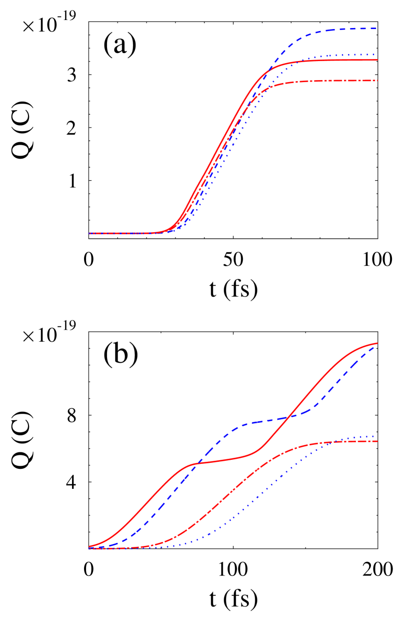
Figure 3: (Color online) Time dependence of charge pumped through the junction Q(t), Eq.(12) for several chirp rates. Shown are results for (a) $\Phi^{\prime\prime}=2000$ and $-2000$ fs² without energy transfer $B(\varepsilon_{21})=0$ (solid line, red and dashed line, blue, respectively), and taking into account energy transfer term $B(\varepsilon_{21})=0.1$ eV (dash-dotted line, red and dotted line, blue, respectively), and (b) $\Phi^{\prime\prime}=10000$ and $-10000$ fs² for $B(\varepsilon_{21})=0.1$ eV and $\mu\mathcal{E}_{0}=0.03$ (solid line, red and dashed line, blue, respectively) and $\mu\mathcal{E}_{0}=0.003$ eV (dash-dotted line, red and dotted line, blue, respectively).

Figure 3 demonstrates pumped charge build-up during the laser pulse excitation. One sees that the local field formation leads to asymmetry in pumped charge for opposite chirp rates. Negatively chirped incoming field creates longer local pulse (see Fig. 2b), which results in increase in total charge pumped through the junction. Role of electron-hole excitations in the contacts on charge buildup is shown in Fig. 3a. Since processes of escape from LUMO into the right contact and energy relaxation on the molecule compete for the excited state population, current (and consequently pumped charge) diminish with increase of coupling to electron-hole excitations in the contacts. Fig. 3b shows effect of intensity of incoming pulse on the transfered charge buildup. For higher intensity the build-up demonstrates saturation in the middle of the pulse. The reason for this behavior is the competition between timescales related to Rabi oscillation induced by local field between molecular levels and electronic escape rate from molecule into contacts ($\sim 1/\Gamma$). On the one hand, both negatively and positively chirped pulses in the middle have frequency approximately at resonance with HOMO-LUMO transition, $\omega\approx\varepsilon_{2}-\varepsilon_{1}$, which is a prerequisite to effective electron transfer and thus increase in pumped charge. On the other hand, at resonance Rabi oscillationsLandau and Lifshitz (1991) at high enough intensities compete with electron escape rate, thus effectively blocking current through the junction. Depending on parameters this may lead either to most effective charge transfer in the middle of the pulse (dash-dotted and dotted lines in panel b), or to suppression of charge transfer at this point (solid and dashed line in panel b). Note that the effect is not related to non-Markov relaxation, i.e. this behavior is observed also in the absence of hybridization between molecule and contact(s) states, and its relation to Landau-Zener problemNitzan (2006) in terms of total charge pumped across the junction was discussed in Ref. Fainberg et al., 2007. Note also, that with positively chirped pulse changing frequency from lower to higher transfered charge buildup is more effective at the start of the pulse (at lower frequencies), while for negatively chirped pulse more effective buildup takes place at the end of the pulse (compare solid and dashed lines in Figs. 3b and 5b). Contrary to buildup suppression in the middle of the pulse, this effect is due to molecule-contact hybridization. The latter leads to broadening of molecular levels, and effectiveness of HOMO-LUMO charge transfer depends (among other conditions) on integral of occupied states at HOMO and empty states at LUMO separated by frequency of incident light $\int dEG^{<}_{11}(E)G^{>}_{22}(E+\omega)$. Clearly, at frequencies below resonance the latter is greater than at frequencies above it.

Figure 4: (Color online) Charge pumped through the junction during pulse vs. chirp rate: (a) total charge, i.e. integral of Q(t), Eq.(12), over local field pulse duration, and (b) asymmetry in charge transfer between positively and negatively chirped incoming laser pulses, $\Delta Q\equiv Q(|\Phi^{\prime\prime}|)-Q(-|\Phi^{\prime\prime}|)$. Shown are results with ($B(\varepsilon_{21})=0.1$eV, dashed line with triangles, blue) and without ($B(\varepsilon_{21})=0$, solid line with circles, red) energy transfer.

Local field asymmetry relative to the sign of the chirp rate in the frequency domain leads to asymmetry in charge pumping contrary to symmetric situation presented in Ref. Fainberg et al., 2007, as is demonstrated in Fig. 4a. One can see that the pumped charge is almost symmetric at high rates with asymmetry confined to the low rate region. Difference between charge pumped through the junction at positive and negative chirp rates is shown in Fig. 4b. As discussed above duration of local field due to positively chirped incoming pulse is shorter than the one due to negatively chirped analog. This compression is the cause of less charge pumped through the system in the former case, which results in decrease in $\Delta Q\equiv Q(\Phi^{\prime\prime})-Q(-\Phi^{\prime\prime})$ in the region of $\Phi^{\prime\prime}(\nu_{0})$ from $0$ to $3000$ fs². Indeed, at the very low rates frequency of the pulse does not change much, so the asymmetry is solely due to difference in pulse length. At a higher rates an additional factor appears: the most effective contribution to charge transfer takes place at a particular region of frequencies (at and just below resonance, as is discussed above). This region is passed quicker in the positively chirped local pulse, and in the region up to $3000$ fs² this results in increase of asymmetry, since negatively chirped pulse spends more time in its effective frequencies zone. Further increase of chirp rate leads to decrease and almost disappearance of the asymmetry. The reason is decrease of ratio of the pulses difference to overall local pulse duration.

Coupling to electron-hole excitations not only diminishes pumped charge (compare solid and dashed lines in panel a), but also decreases asymmetry (panel b). The latter results from the fact that rate for molecular energy relaxation (LUMO ${}\to{}$ HOMO transition due to coupling to excitations in the contacts) is proportional to population in the LUMO (see discussion in Ref. Galperin and Nitzan, 2006). So for higher currents also energy relaxation will be more efficient, thus effectively compensating for the difference.

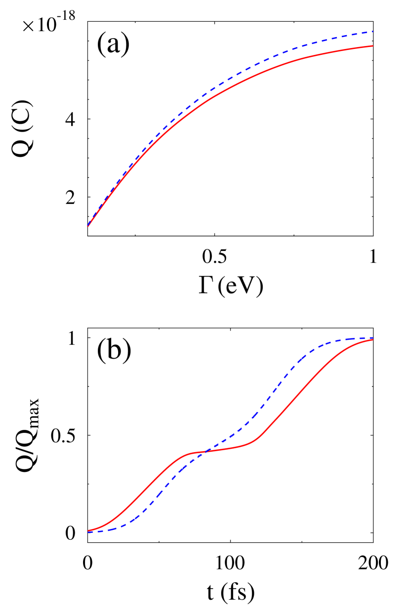
Figure 5: (Color online) Dependence of charge pumping on molecule-contact states hybridization at $\mu\mathcal{E}_{0}=0.03$eV. Shown are (a) Charge pumped through the junction during pulse vs. electronic escape rate for chirp rate $\Phi^{\prime\prime}=10000$ fs² (solid line, red) and $-10000$ fs² (dashed line, blue), and (b) Normalized transferred charge build-up (charge normalized to total charge transferred during the pulse) vs. time for chirp rate $\Phi^{\prime\prime}=10000$ fs² and $\Gamma^{L}_{11}=\Gamma^{R}_{22}=0.1$eV (solid line, red) and $1$eV (dashed line, blue). Red line in panel (b) is the same as solid red line in Fig. 3b.

Importance of non-Markov behavior for charge pump is demonstrated in Figure 5. Fig. 5a shows pumped charge as function of level width (for two opposite choices of chirp rate). Increase in total charge pumped through the junction with increase in hybridization saturates at high strength of coupling between molecule and contacts. Such behavior is expected: at low hybridization there is only one frequency corresponding to resonance, where pumping is most effective, so only an ’instant’ of chirped pulse contributes to charge transfer. As molecule-contact coupling grows the condition of resonance transition becomes less and less strict. Eventually any frequency within the chirped pulse has roughly same effectiveness – this is the reason for saturation. Also, stronger coupling means more effective molecule-contact electron transfer, which competes more effectively with intra-molecular Rabi oscillation at resonance. This competition is demonstrated in Fig. 5b, where middle-of-the-pulse saturation (see discussion of Fig. 3) disappears for stronger molecule-contact coupling.

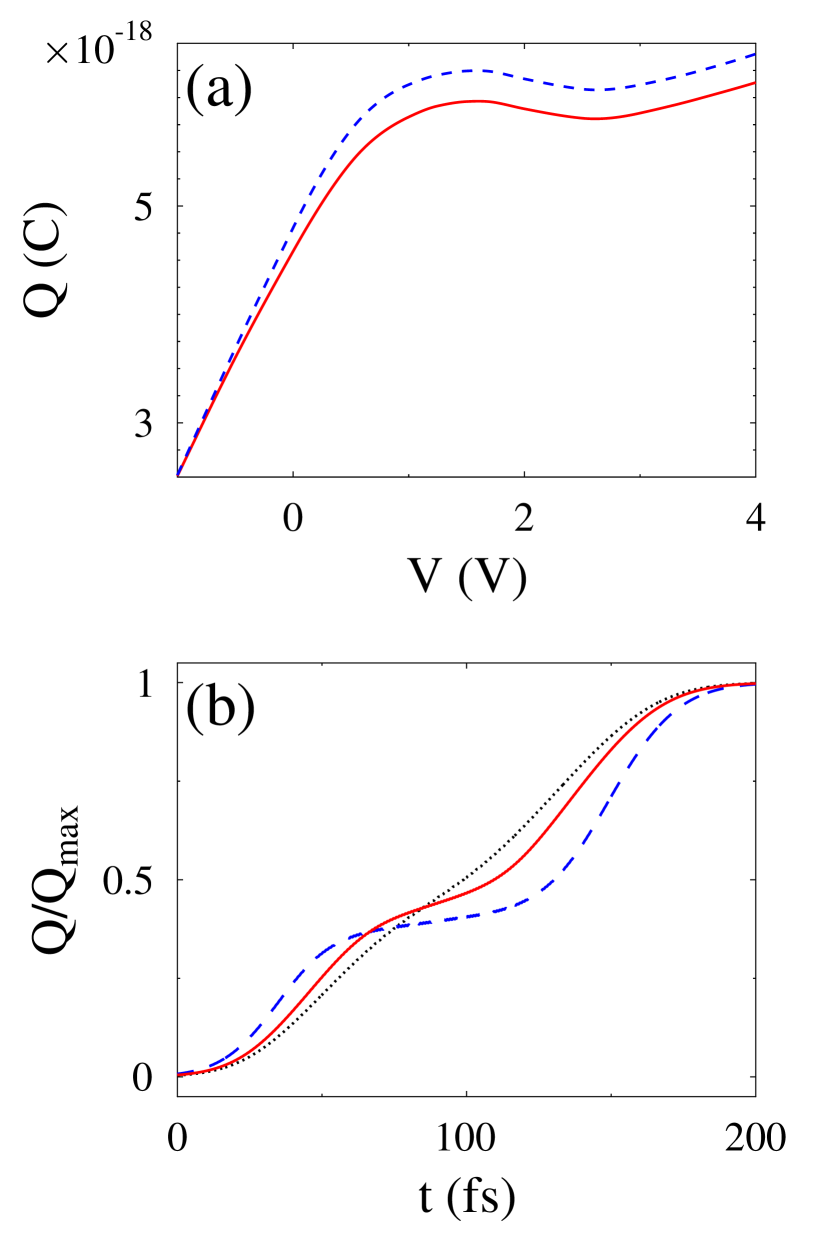
Figure 6: (Color online) Dependence of charge pumping on bias. (a) Total excess charge pumped through the junction during pulse vs. bias for chirp rate $\Phi^{\prime\prime}=10000$ fs² (solid line, red) and $-10000$ fs² (dashed line, blue). (b) Excess charge build-up (normalized to total excess charge transferred during the pulse) vs. time at chirp rate $\Phi^{\prime\prime}=10000$ fs² for $V_{sd}=-1$V (dashed line, blue), $0$V (solid line, red), and $1$ V (dotted line, black). Here $\Gamma^{L}_{11}=\Gamma^{R}_{22}=0.5$ eV. Red line in panel (b) is the same as solid red line in Fig. 3b.

Finally, in Figure 6 we discuss influence of bias on charge pumping. Here we define optically pumped charge (excess charge) as a difference between charge pumped through the junction with and without laser field. Fig. 6a demonstrates total excess pumped charge during laser pulse for opposite choices of chirp rate as function of bias. Application of bias has 2 effects on the pumping process: 1. it depletes (populates) the HOMO (the LUMO) and 2. it may block or release channels for electron transfer from LUMO to contact $R$. This leads to a situations when most effective optical pumping does not correspond to zero bias, rather we see shallow peak at $V\sim 1$V. Explanation is related to the fact that broadened molecular levels are essentially a set of scattering channels with different transmission probabilities: high conducting channels are in the center of Lorentzian, while channels in the sides of distribution are poor conductors. Optical process takes electron from an occupied ground state and puts it into one of empty excited state. Effectiveness of the charge pump is defined by increase or decrease of current through the junction under optical pulse (see discussion in Ref. Sukharev and Galperin, 2010). In particular, negative bias decreases effectiveness of the pump mostly due to blocking part of LUMO-$R$ escape routes. Positive bias opens additional escape routes at the tail of LUMO Lorentzian, facilitating increase in pump efficiency. However, additional effect of depleting HOMO and populating LUMO partially blocks optically induced HOMO-LUMO electron transfer, thus reducing overall effectiveness of optical pumping. Competition between the two proceses reveals itself as a shallow peak at $\sim 1$V.

Time resolved charge buildup is presented in Fig 6b. Middle-of-the-pulse saturation observed previously at equilibrium (solid line, same as in Fig. 3b) is enhanced at negative (dashed line) and disappears at positive bias (dotted line). The reason is similar to competition between Rabi frequency and escape rate discussed above. Indeed, with negative bias partially blocking fast escape route for the electron from excited state into right contact, Rabi oscillation plays an important role at quasi-resonant situation in the middle of the pulse. Positive opening additional routes makes Rabi oscillation less effective.

VII Conclusion

We consider a two-level (HOMO-LUMO) model for optically-driven molecular charge pump. Such pump may be realized as a junction formed by a molecule with strong charge-transfer transition between its ground and excited states. The junction is driven by both applied bias and laser pulse. The latter is treated as an external classical driving force.

Our consideration is the generalization of previous studyFainberg et al. (2007) which takes into account effects of local field (‘hot spot’ formation) and hybridization between the states of molecule and contact(s) (non-Markov effects). We formulate approximate closed set of EOMs for single- and two-particle GFs. Electron transfer in the former is treated exactly. To close set of equations the latter are considered within Markov approximation. Our EOMs are reduced to set of equation derived in Ref. Fainberg et al., 2007 under several simplifying assumptions: weak molecule-contact coupling (neglect of hybridization), neglect of non-diagonal terms in molecular spectral function, and within rotating wave approximation.

Incoming laser pulse is assumed to be linearly chirped. Local field is calculated within FDTD technique on a grid with bowtie antenna geometry used to represent junction metallic contacts. We find that contrary to symmetric behavior of the pump relative to sign of the chirp rate, duration of the corresponding local field pulse depends on the sign of incoming chirp, which results in asymmetric operation of the pump. The asymmetry depends on the incoming pulse chirp rate in a non-monotonic manner. Junction response to optical driving is symmetric to both low and high chirp rates, going through a maximum between the two extremes. We find that this behavior is caused by the correspondence between pulse duration of the local field and detuning of its frequency at the end of the pulse from energy difference between molecular states ($\varepsilon_{2}-\varepsilon_{1}$).

We note that at quasi-resonance charge pump becomes ineffective, due to the competition between intra-molecular Rabi oscillation induced by the pulse with electron transfer from molecule to contact. Increase of the molecule-contact coupling strength increases electron escape rate, thus reducing ineffectiveness of the pump due to Rabi oscillations.

Also we study the effect of bias on optically-facilitated charge transfer through the junction. We find that in the non-Markov situation (i.e. when hybridization between molecule and contacts is non-negligible) most effective charge pump regime is at finite positive bias, rather than at equilibrium as one may expect from Markov consideration of Ref. Fainberg et al., 2007. The effect comes from optically-assisted charge redistribution between low and high conducting scattering channels in broadened molecular states, as was discussed in our previous publication.Sukharev and Galperin (2010) Within the model negative bias reduces (positive increases) excess charge pumping due to blocking (facilitating) outgoing scattering channels in the excited molecular state and thus increasing (decreasing) the role of intra-molecular Rabi oscillations.

Finally, direct electron-hole excitation in contacts, heating, and inelastic effects are examples of effects beyond current consideration which may also have a significant impact on the properties of a molecular charge pump.

Appendix A Derivation of Eq.(13)

EOM for (13) in contour variable $\tau$ starts from writing Heisenberg equation for $\hat{d}_{m}(\tau)$

$$i\frac{\partial}{\partial\tau}G_{mm^{\prime}}(\tau,\tau^{\prime})=\delta_{m,m^{\prime}}\delta(\tau,\tau^{\prime})+\varepsilon_{m}G_{mm^{\prime}}(\tau,\tau^{\prime})$$

$$-\mu E(t)G_{\bar{m}m^{\prime}}(\tau,\tau^{\prime})+V_{mk}G_{km^{\prime}}(\tau,\tau^{\prime})$$ (24)

$$+\sum_{k_{1}\neq k_{2}}V^{en}_{k_{1}k_{2}}\mathcal{G}_{\bar{m}k_{2},m^{\prime}k_{1}}(\tau-,\tau;\tau^{\prime},\tau+)$$

The last two terms on the right come from electron and energy transfer terms in Eq.(II). Treating the two within non-crossing approximation allows to find the first exactly within a standard procedureHaug and Jauho (1996)

$$G_{km^{\prime}}(\tau,\tau^{\prime})=\sum_{m_{1}}\int_{c}d\tau_{1}g_{k}(\tau,\tau_{1})V_{km_{1}}G_{m_{1}m^{\prime}}(\tau_{1},\tau^{\prime})$$ (25)

Two particle Green function in the second term is treated (still keeping non-crossing approximation in mind) within first order perturbation theory in energy transfer

$$\mathcal{G}_{\bar{m}k_{2},m^{\prime}k_{1}}(\tau,\tau;\tau^{\prime},\tau)=-iV^{en}_{k_{2}k_{1}}\times$$ (26)

$$\quad\sum_{m_{1}}\int_{c}d\tau_{1}g_{k_{2}}(\tau,\tau_{1})g_{k_{1}}(\tau_{1},\tau)\mathcal{G}_{\bar{m}\bar{m}_{1},m^{\prime}m_{1}}(\tau,\tau_{1};\tau^{\prime},\tau_{1}+)$$

Substituting (25) and (26) into (A) yields (13).

Eq.(17) is retarded projection of Eq.(13) with omitted energy transfer term. The approximation is based on an estimate that in usual situation electron escape rate should be much bigger than corresponding energy transfer, $\Gamma\gg B$.Galperin et al. (2006)

Eqs. (18) and (19) is lesser projection of (13) taken at equal times, $-i\mathbf{G}^{<}(t,t)$. Note that (19) is exact, while in (18) we employ Markov approximation in derivation of the energy transfer term similar to previous publications,Galperin and Nitzan (2006); Fainberg et al. (2007) for example

$$\sum_{k_{1}\neq k_{2}}\sum_{m_{1}}\int_{-\infty}^{t}dt_{1}g_{k_{2}}^{>}(t-t_{1})g_{k_{1}}^{<}(t_{1}-t)$$

$$\qquad\times\left\langle\hat{d}_{m}^{\dagger}(t)\hat{d}_{\bar{m}}(t)\hat{d}_{m_{1}}^{\dagger}(t_{1})\hat{d}_{\bar{m}_{1}}(t_{1})\right\rangle$$

$$\approx\int_{-\infty}^{t}dt_{1}g_{k_{2}}^{>}(t-t_{1})g_{k_{1}}^{<}(t_{1}-t)e^{i(\varepsilon_{m_{1}}-\varepsilon_{\bar{m}_{1}})(t_{1}-t)}$$ (27)

$$\qquad\times\left\langle\hat{d}_{m}^{\dagger}(t)\hat{d}_{\bar{m}}(t)\hat{d}_{m_{1}}^{\dagger}(t)\hat{d}_{\bar{m}_{1}}(t)\right\rangle$$

$$\approx[1-n_{k_{2}}]n_{k_{1}}\pi\delta\left(\varepsilon_{k_{2}}-\varepsilon_{k_{1}}+\varepsilon_{m_{1}}-\varepsilon_{\bar{m}_{1}}\right)$$

$$\qquad\times\left\langle\hat{d}_{m}^{\dagger}(t)\hat{d}_{\bar{m}}(t)\hat{d}_{m_{1}}^{\dagger}(t)\hat{d}_{\bar{m}_{1}}(t)\right\rangle$$

Using (A) and similar expressions for other parts of the Keldysh contour deformed in accordance with Langreth rulesHaug and Jauho (1996) in the energy transfer term of lesser projection of diagonal element of (13), and utilizing (V) leads to (18).

Finally, Eq.(20) is treated with Markov approximation (see Eq.(A) above) applied to both electron and energy transfer terms. Then the derivation goes along the lines presented in Ref Fainberg et al., 2007.

Appendix B Markov limit of Eqs. (17)-(20)

EOMs derived in Ref. Fainberg et al., 2007 are Markov limit of Eqs.(18)-(20) within static quasiparticle approximation assumed for molecular states. The latter implies disregarding Eq.(17), and assuming instead

$$i\left[G^{r}_{mm^{\prime}}(t,E)-G^{a}_{mm^{\prime}}(t,E)\right]=2\pi\delta_{m,m^{\prime}}\delta(E-\varepsilon_{m})$$ (28)

Then, disregarding level mixing due to coupling to contacts $\Gamma^{K}_{12}=\Gamma^{K}_{21}=0$, Eqs. (18) and (19) reduce to Eqs. (33) and (34) of Ref. Fainberg et al., 2007. After omitting non-diagonal elements of self-energy in Eq.(20) one gets Eq.(35) of Ref. Fainberg et al., 2007.

References

- Hänggi (2011) P. Hänggi, Nature Materials 10, 6 (2011).
- Roeling et al. (2011) E. M. Roeling, W. C. Germs, B. Smalbrugge, E. J. Geluk, T. de Vries, R. A. J. Janssen, and M. Kemerink, Nature Materials 10, 51 (2011).
- Siegle et al. (2010) V. Siegle, C.-W. Liang, B. Kaestner, H. W. Schumacher, F. Jessen, D. Koelle, R. Kleiner, and S. Roth, Nano Letters 10, 3841 (2010).
- Hanson et al. (2007) R. Hanson, L. P. Kouwenhoven, J. R. Petta, S. Tarucha, and L. M. K. Vandersypen, Rev. Mod. Phys. 79, 1217 (2007).
- Bogani and Wernsdorfer (2008) L. Bogani and W. Wernsdorfer, Nature Materials 7, 179 (2008).
- Nitzan (2007) A. Nitzan, Science 317, 759 (2007).
- Wang et al. (2007) Z. Wang, J. A. Carter, A. Lagutchev, Y. K. Koh, N.-H. Seong, D. G. Cahill, and D. D. Dlott, Science 317, 787 (2007).
- Halas (2010) N. J. Halas, Nano Letters 10, 3816 (2010).
- Hildner et al. (2011) R. Hildner, D. Brinks, and N. F. van Hulst, Nature Physics 7, 172 (2011).
- Gordon et al. (1999) R. J. Gordon, L. Zhu, and T. Seideman, Accounts of Chemical Research 32, 1007 (1999).
- Ward et al. (2007) D. R. Ward, N. K. Grady, C. S. Levin, N. J. Halas, Y. Wu, P. Nordlander, and D. Natelson, Nano Letters 7, 1396 (2007).
- Ward et al. (2008) D. R. Ward, N. J. Halas, J. W. Ciszek, J. M. Tour, Y. Wu, P. Nordlander, and D. Natelson, Nano Letters 8, 919 (2008).
- Ioffe et al. (2008) Z. Ioffe, T. Shamai, A. Ophir, G. Noy, I. Yutsis, K. Kfir, O. Cheshnovsky, and Y. Selzer, Nature Nanotechnology 3, 727 (2008).
- Ward et al. (2011) D. R. Ward, D. A. Corley, J. M. Tour, and D. Natelson, Nature Nanotechnology 6, 33 (2011).
- Kohler et al. (2004) S. Kohler, S. Camalet, M. Strass, J. Lehmann, G.-L. Ingold, and P. Hänggi, Chemical Physics 296, 243 (2004).
- Galperin et al. (2006) M. Galperin, A. Nitzan, and M. A. Ratner, Physical Review Letters 96, 166803 (2006).
- Viljas et al. (2007) J. K. Viljas, F. Pauly, and J. C. Cuevas, Physical Review B 76, 033403 (2007).
- Viljas et al. (2008) J. K. Viljas, F. Pauly, and J. C. Cuevas, Physical Review B 77, 155119 (2008).
- Galperin and Nitzan (2005) M. Galperin and A. Nitzan, Physical Review Letters 95, 206802 (2005).
- Galperin and Nitzan (2006) M. Galperin and A. Nitzan, Journal of Chemical Physics 124, 234709 (2006).
- Harbola et al. (2006) U. Harbola, J. B. Maddox, and S. Mukamel, Physical Review B 73, 075211 (2006).
- Galperin and Tretiak (2008) M. Galperin and S. Tretiak, Journal of Chemical Physics 128, 124705 (2008).
- Sukharev and Galperin (2010) M. Sukharev and M. Galperin, Physical Review B 81, 165307 (2010).
- Galperin et al. (2009a) M. Galperin, M. A. Ratner, and A. Nitzan, Nano Letters 9, 758 (2009a).
- Galperin et al. (2009b) M. Galperin, M. A. Ratner, and A. Nitzan, Journal of Chemical Physics 130, 144109 (2009b).
- Ponder and Mathies (1983) M. Ponder and R. Mathies, The Journal of Physical Chemistry 87, 5090 (1983).
- Colvin and Alivisatos (1992) V. L. Colvin and A. P. Alivisatos, The Journal of Chemical Physics 97, 730 (1992).
- Smirnov and Braun (1998) S. N. Smirnov and C. L. Braun, Review of Scientific Instruments 69, 2875 (1998).
- Fainberg et al. (2007) B. D. Fainberg, M. Jouravlev, and A. Nitzan, Physical Review B 76, 245329 (2007).
- Allen and Eberly (1975) L. Allen and J.-H. Eberly, Optical resonance and two-level atoms (John Wiley & Sons, New York, London, Sydney, Toronto, 1975).
- Bryllert et al. (2002) T. Bryllert, M. Borgstrom, T. Sass, B. Gustafson, L. Landin, L. E. Wernersson, W. Seifert, and L. Samuelson, Applied Physics Letters 80, 2681 (2002).
- Sanchez et al. (2008) R. Sanchez, G. Platero, and T. Brandes, Physical Review B 78, 125308 (2008).
- Li et al. (2010) G. Q. Li, B. D. Fainberg, A. Nitzan, S. Kohler, and P. Hänggi, Physical Review B 81, 165310 (2010).
- Taflove and Hagness (2005) A. Taflove and S. C. Hagness, Computational Electrodynamics: The Finite-Difference Time-Domain Method (Artech House, Boston, 2005).
- Stockman et al. (2004) M. I. Stockman, D. J. Bergman, and T. Kobayashi, Physical Review B 69, 054202 (2004).
- Lee and Gray (2005) T.-W. Lee and S. K. Gray, Physical Review B 71, 035423 (2005).
- Aeschlimann et al. (2007) M. Aeschlimann, M. Bauer, D. Bayer, T. Brixner, F. J. Garcia de Abajo, W. Pfeiffer, M. Rohmer, C. Spindler, and F. Steeb, Nature 446, 301 (2007).
- Cao et al. (2010) L. Cao, R. A. Nome, J. M. Montgomery, S. K. Gray, and N. F. Scherer, Nano Letters 10, 3389 (2010).
- Weiner (2009) A. M. Weiner, Ultrafast optics (John Wiley and Sons, Hoboken, New Jersey, 2009).
- Jauho et al. (1994) A. P. Jauho, N. S. Wingreen, and Y. Meir, Phys. Rev. B 50, 5528 (1994).
- Galperin et al. (2007) M. Galperin, A. Nitzan, and M. A. Ratner, Physical Review B 76, 035301 (2007).
- Landau and Lifshitz (1991) L. D. Landau and E. M. Lifshitz, Quantum Mehcanics. Non-relativistic Theory. (Pergamon Press, 1991).
- Nitzan (2006) A. Nitzan, Chemical Dynamics in Condensed Phases (Oxford University Press, 2006).
- Haug and Jauho (1996) H. Haug and A.-P. Jauho, Quantum Kinetics in Transport and Optics of Semiconductors, vol. 123 (Springer-Verlag, Berlin Heidelberg, 1996).