Continuous-variable controlled-$Z$ gate using an atomic ensemble

Abstract

The continuous-variable controlled-$Z$ gate is a canonical two-mode gate for universal continuous-variable quantum computation. It is considered as one of the most fundamental continuous-variable quantum gates. Here we present a scheme for realizing continuous-variable controlled-$Z$ gate between two optical beams using an atomic ensemble. The gate is performed by simply sending the two beams propagating in two orthogonal directions twice through a spin-squeezed atomic medium. Its fidelity can run up to one if the input atomic state is infinitely squeezed. Considering the noise effects due to atomic decoherence and light losses, we show that the observed fidelities of the scheme are still quite high within presently available techniques.

PACS numbers

03.67.Lx, 03.67.Bg, 42.50.Dv

I introduction

Quantum computation (QC) is one of the most fascinating and fruitful area of research. It strives to utilize the principles of quantum mechanics to improve the efficiency of computation. In recent years, with the discoveries of many quantum algorithms Shor (1997); Grover (1997), QC has been shown to work faster than any known classic computation. Though originally based upon discrete variables (DV), QC over continuous variables (CV) has also been addressed by Lloyd and Braunstein Lloyd and Braunstein (1999). In analogy to DV QC based on gate operations, universal CV QC can be carried out by executing a finite set of CV quantum logic gates, including displacement gate, shearing gate, cubic phase gate, and controlled-$Z$ ($C_{Z}$) gate Gu et al. (2009).

CV $C_{Z}$ gate [also called as quantum nondemolition (QND) gate] is a canonical two-mode gate, which is a CV analog of a two-qubit CPHASE gate. Like the DV CPHASE gate, CV $C_{Z}$ gate is considered as one of the most fundamental CV quantum gates. Nowadays, much effort has been devoted to the realization of such gate in many physical systems, especially in optical systems Grangier et al. (1998); Levenson et al. (1986); Grangier and Roch (1989); Holland et al. (1990); Grangier et al. (1991); La Porta et al. (1989); Braunstein (2005); Filip et al. (2005); Yoshikawa et al. (2008). However, by now optical CV CZ gate is still experimentally challenging. Initial approaches to realize optical QND interactions are based on nonlinear optical systems Levenson et al. (1986); Grangier and Roch (1989); Holland et al. (1990); Grangier et al. (1991); La Porta et al. (1989). $C_{Z}$ gate is performed by simply sending the beams through an optical crystal or an optical fiber. These approaches, however, are hampered by the weak nonlinearities in the nonlinear media. Although the nonlinearities can be enhanced by embedding the crystal inside a cavity or using a long fiber, such enhancement techniques, on the other hand, make it difficult to inject the light states into the system and cause large loss rates. Recently, an alternative approach was proposed to circumvent cumbersome nonlinear interactions by using only linear optical elements and off-line squeezed light beams Filip et al. (2005). This approach, however, requires efficient homodyne detection techniques and accurate feed forward control, which poses a challenge to the experimental realization Yoshikawa et al. (2008). In recent years, with the emergence of one-way QC Menicucci et al. (2006), the interest in theoretical and experimental realization of optical $C_{Z}$ gate is further fuelled.

One-way QC is a new form of QC which eliminates unitary evolution and relies solely on adaptive measurements on a suitably prepared multiparty entangled state. This model is quite attractive because local projective measurements are often easier to implement than unitary evolution. Most of the challenging work of QC are then converted into the problem of creating the multiparty entangled state—the so-called cluster state. Cluster state in the CV regime is a multimode squeezed Gaussian state and has been proved universal resources for CV one-way QC. To date, several methods have been proposed to construct such state. One of them is called the canonical method Zhang and Braunstein (2006), which involves offline single-mode squeezers and $C_{Z}$ gates. Although this method is conceptually simple, it is not very practical because of the experimental challenges associated with $C_{Z}$ gates. Shortly after this method, another method, linear-optics method van Loock et al. (2007), has also been proposed to eliminate the need for $C_{Z}$ gates. Any desired CV cluster state can be created by using only offline-squeezing and linear optics. This method, however, suffers from drawback that effects its scalability. Recently, Menicucci et al. proposed the single-QND-gate method Menicucci et al. (2010) which reintroduces the $C_{Z}$ gates. Although this method has many distinct advantages, i.e. it saves the resources needed greatly and eliminates the need for long-time coherence of a large cluster state, still the inefficiency of the experimental realization of $C_{Z}$ gates casts it into the shade. Apparently, the only way to repolish the $C_{Z}$-based methods (and thus the CV one-way QC) is to devise many new schemes which enable us to implement the $C_{Z}$ gate more efficiently.

In this paper, we propose a simple and practical scheme to realize optical $C_{Z}$ gate using a free-space macroscopic atomic ensemble. We show that $C_{Z}$ gate between two optical beams can be performed by simply sending them perpendicularly to each other twice through a spin-squeezed atomic ensemble, see Fig. 1(a). The fidelities obtained in the scheme depend solely on the degree of the atomic squeezing. The more the amount of squeezing input, the higher the fidelity obtain. Near-unity fidelity can be achieved under the condition that the atomic state is infinitely squeezed. Unlike previous measurement-based schemes Yoshikawa et al. (2008); Filip et al. (2005); *PhysRevA.80.050303, our scheme requires neither homodyne detection nor feedforward control during the gate operation, which greatly simplifies its experimental implementation. Within the presently experimentally available parameters, we find that the observed fidelities are quite high even with room-temperature atomic vapors.

The remainder of this paper is organized as follows. In sec. ii@ we first review some basic theories, and then give details of $C_{Z}$ operation based on an atomic ensemble. In sec. iii@ we will consider the noise effects. After that, the experimental feasibility of the scheme is also discussed. Finally, sec. iv@ contains brief conclusions.

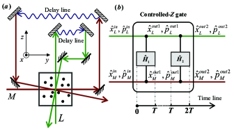
Figure 1: (Color online) (a) Scheme setup for realization of optical $C_{Z}$ gate in an atomic ensemble. Two light beams $L$ and $M$ simultaneously enter a spin-squeezed atomic ensembles. The outgoing beams then pass through a delay line. After the whole of the beams run through the atomic sample, they enter the ensemble again. When the beams exit, a $C_{Z}$ gate between $L$ and $M$ is performed. (b) Schematic chart of the $C_{Z}$ gate. The two interactions do not overlap in the time line. After them, the gate is performed.

II BASIC THEORY AND CONTROLLED-Z Gate

II.1 Basic theory

For a two-mode two-party system described by the quadrature operators $\hat{x}_{1,2}$ and $\hat{p}_{1,2}$ satisfying the commutation relation $[\hat{x}_{j},\hat{p}_{k}]=i\delta_{jk}$, the QND-gate coupling Hamiltonian can be written as: $\hat{H}_{QND}=\hbar\chi\hat{p}_{1}\hat{p}_{2}$, where $\chi$ is the coupling coefficient. In the Heisenberg picture, one may deduce the ideal QND input-output relations for both position and momentum operators

$$\hat{x}_{1}^{out}=\hat{x}_{1}^{in}+G\hat{p}_{2}^{in},~{}~{}~{}\hat{p}_{1}^{out}=\hat{p}_{1}^{in},\hfill$$

$$\hat{x}_{2}^{out}=\hat{x}_{2}^{in}+G\hat{p}_{1}^{in},~{}~{}~{}\hat{p}_{2}^{out}=\hat{p}_{2}^{in},$$ (1)

where $G=\chi t$ is the gain of the interaction, and $t$ represents the interaction time. For nonzero $G$, these equations imply that the two sub-systems become Gaussian entangled Braunstein and van Loock (2005). Such entanglement has been widely used in quantum information processing Kuzmich and Polzik (2000); Duan et al. (2000); Massar and Polzik (2003). Specifically, if we put the gain of the interaction $G=1$, then we obtain the CV $C_{Z}$ gate as desired.

To realize optical $C_{Z}$ gate in an atomic ensemble, let us first investigate the interaction between light and atoms. Consider a cell filled with a large number of atoms interacting with a light pulse traveling along the $z$ direction. The atoms in the cell are initially prepared in a coherent spin state, i.e. a fully polarized state along the $x$ axis. As a result, we may treat the $x$ component of the collective spin as a $c$ number, that is $\hat{J}_{x}$ by $J_{x}$. In this case, we can map the transverse spin components into dimensionless canonical variables $(\hat{x}_{a},\hat{p}_{a})=(\hat{J}_{y},\hat{J}_{z})/\sqrt{J_{x}}$ obeying $[\hat{x}_{a},\hat{p}_{a}]=i$. The light pulse interacting with atoms is also linearly polarized along the $x$ axis. Similarly, we may define the optical canonical operators as $(\hat{x}_{ph}(t),\hat{p}_{ph}(t))=(\hat{S}_{y}(t),\hat{S}_{z}(t))/\sqrt{S_{x}}$, which satisfy the commutation relation $[\hat{x}_{ph}(t),\hat{p}_{ph}(t)]=i\delta(t-t^{\prime})$ and have the dimensions of $1/\sqrt{time}$, where $\hat{S}_{i}$ (with $i\in\{x,y,z\}$) denotes the time dependent Stokes vector component. Under the condition that the frequency of the beam was tuned far off resonance with atomic transition Kuzmich et al. (1998), the interaction of light with atoms can be described by the effective Hamiltonian $\hat{H}=\tilde{\kappa}_{0}\hat{p}_{ph}\hat{p}_{a}$, with $\tilde{\kappa}_{0}=a\sqrt{J_{x}S_{x}}$, where $a$ is the effective coupling strength Kuzmich and Polzik (2000); Kuzmich et al. (1998). Obviously, it is a QND-type. An important, immediate application of this Hamiltonian is quantum memory Julsgaard et al. (2004). However, initially, such interactions were extensively investigated to produce spin squeezing Kuzmich et al. (1998); Takahashi et al. (1999); *PhysRevA.60.2346.

We here briefly review the process of spin squeezing based on QND detection. Following Eq. (1) the input-output relations for light and atoms can be directly derived as: $\hat{x}_{ph}^{out}=\hat{x}_{ph}^{in}+\kappa_{0}\hat{p}_{a}^{in},\hat{p}_{ph}^{out}=\hat{p}_{ph}^{in},\hat{x}_{a}^{out}=\hat{x}_{a}^{in}+\kappa_{0}\hat{p}_{ph}^{in},\hat{p}_{a}^{out}=\hat{p}_{a}^{in}$, with $\kappa_{0}=\tilde{\kappa}_{0}\sqrt{T}$, where $T$ is the duration of the pulse. Next, a measurement of $\hat{x}_{ph}^{out}$ is performed, giving a random measurement outcome $\xi$. The momentum operator $\hat{p}_{a}^{out}$ is then displaced by an amount $g\xi$, where $g$ is a gain factor, resulting in $\hat{p}_{a}^{out}=\hat{p}_{a}^{in}-gx_{ph}^{out}=({1-g\kappa_{0}})\hat{p}_{a}^{in}+g\hat{x}_{ph}^{in}$. If the light pulse is initially in coherent state such that $\Delta{x_{ph}^{in}}^{2}=\Delta{p_{ph}^{in}}^{2}=1/2$, the variance of $\hat{p}_{a}^{out}$ can be easily calculated, giving $(\Delta{\hat{p}_{a}^{out}})^{2}=\frac{1}{2}[{({1-g\kappa_{0}})^{2}+g^{2}}].$ Optimizing it, we get $(\Delta{\hat{p}_{a}^{out}})^{2}=\frac{1}{2}\frac{1}{1+\kappa_{0}^{2}}$ for $g=\kappa_{0}/{(1+\kappa_{0}^{2})}$. Obviously, for nonzero $\kappa_{0}$, the atomic momentum operator is then squeezed. Finally, we obtain the squeezed spin state (SSS) as:

$$\hat{x}_{a}^{out}=\sqrt{1+\kappa_{0}^{2}}\hat{x}_{a}^{in},~{}~{}~{}\hat{p}_{a}^{out}=\frac{1}{\sqrt{1+\kappa_{0}^{2}}}\hat{p}_{a}^{in}.$$ (2)

II.2 Controlled-Z gate

Let us now consider the implementation of optical $C_{Z}$ gate in an atomic ensemble. Suppose that we have an atomic ensemble prepared in the SSS described above, through which two $x$-polarized light beams are transmitted simultaneously from two perpendicular directions, see Fig. 1(a). For the beam $L$ propagating along the $z$ direction, its interaction with atoms can then be described by $\hat{H}_{L}=\tilde{\kappa}_{L}\hat{p}_{L}\hat{p}_{a}$. The second beam $M$ propagates along the $y$ direction, leading to the second Hamiltonian $\hat{H}_{M}=\tilde{\kappa}_{M}\hat{p}_{M}\hat{x}_{a}$ Fiurášek et al. (2006); Muschik et al. (2006). Thus, the complete Hamiltonian for this process can be written as

$$\hat{H}_{1}=\tilde{\kappa}\hat{p}_{L}\hat{p}_{a}+\tilde{\kappa}\hat{p}_{M}\hat{x}_{a},$$ (3)

where we have assumed $\tilde{\kappa}_{L}=\tilde{\kappa}_{M}=\tilde{\kappa}$. Corresponding to this Hamiltonian, one may straightly derive the Heisenberg equations for atoms and the Maxwell-Bloch equations (neglecting the effects of light retardation) for light as Fiurášek et al. (2006); Muschik et al. (2006):

$$\partial_{t}\hat{x}_{a}\left(t\right)=\tilde{\kappa}\hat{p}_{L}^{in}\left(t\right),$$ (4)

$$\partial_{t}\hat{p}_{a}\left(t\right)=-\tilde{\kappa}\hat{p}_{M}^{in}\left(t\right),$$ (5)

$$\hat{x}_{L}^{out1}\left(t\right)=\hat{x}_{L}^{in}\left(t\right)+\tilde{\kappa}\hat{p}_{a}\left(t\right),$$ (6)

$$\hat{p}_{L}^{out1}\left(t\right)=\hat{p}_{L}^{in}\left(t\right),$$ (7)

$$\hat{x}_{M}^{out1}\left(t\right)=\hat{x}_{M}^{in}\left(t\right)+\tilde{\kappa}\hat{x}_{a}\left(t\right),$$ (8)

$$\hat{p}_{M}^{out1}\left(t\right)=\hat{p}_{M}^{in}\left(t\right),$$ (9)

where $\partial_{t}$ stands for the partial derivative with respect to $t$. Equations (4) and (5) can be readily solved by integrating over $t$ on both sides, giving

$$\hat{x}_{a}\left(t\right)=\hat{x}_{a}\left(0\right)+\tilde{\kappa}\int_{0}^{t}{\hat{p}_{L}^{in}\left(\tau\right)}d\tau,$$

$$\hat{p}_{a}\left(t\right)=\hat{p}_{a}\left(0\right)-\tilde{\kappa}\int_{0}^{t}{\hat{p}_{M}^{in}\left(\tau\right)d\tau}.$$ (10)

Inserting this set of equations into Eqs. (6) and (8), one will obtain the expressions for $\hat{x}_{L,M}^{out1}$,

$$\hat{x}_{L}^{out1}\left(t\right) = \hat{x}_{L}^{in}\left(t\right)+\tilde{\kappa}\hat{p}_{a}\left(0\right)-\tilde{\kappa}^{2}\int_{0}^{t}{\hat{p}_{M}^{in}\left(\tau\right)d\tau},$$

$$\hat{x}_{M}^{out1}\left(t\right) = \hat{x}_{M}^{in}\left(t\right)+\tilde{\kappa}\hat{x}_{a}\left(0\right)+\tilde{\kappa}^{2}\int_{0}^{t}{\hat{p}_{L}^{in}\left(\tau\right)}d\tau.$$ (11)

Next, we define the dimensionless collective light modes $\hat{x}_{j}=\int_{0}^{T}{f(t)\hat{x}_{j}(t)dt}$ ($j\in\{L,M\}$) with $[\hat{x}_{j},\hat{p}_{j}]=i$, where $f(t)$ is a temporal mode function specifying the mode in question. For the symmetric mode with $f(t)=1/\sqrt{T}$, Eqs. (11) are then changed into

$$\hat{x}_{L}^{out1} = \hat{x}_{L}^{in}+\kappa\hat{p}_{a}\left(0\right)-\frac{\kappa^{2}}{T^{3/2}}\int_{0}^{T}{\left(T-t\right)\hat{p}_{M}^{in}\left(t\right)dt},$$

$$\hat{x}_{M}^{out1} = \hat{x}_{M}^{in}+\kappa\hat{x}_{a}\left(0\right)+\frac{\kappa^{2}}{T^{3/2}}\int_{0}^{T}{\left(T-t\right)\hat{p}_{L}^{in}\left(t\right)dt},$$

where we have interchanged the order of the double integral and defined the dimensionless coupling strength $\kappa=\tilde{\kappa}\sqrt{T}$. Eqs. (LABEL:equ:6) indicate that, besides the momentum operators $\hat{p}_{M}^{in}$ and $\hat{p}_{L}^{in}$, the position operators $\hat{x}_{L}^{out1}$ and $\hat{x}_{M}^{out1}$ also pick up the information of the input atomic operators $\hat{p}_{a}(0)$ and $\hat{x}_{a}(0)$. Such information bring unfavorable influence on our scheme, since, for an ideal optical $C_{Z}$ gate, only the information of $\hat{p}_{M}^{in}$ and $\hat{p}_{L}^{in}$ are allowed to be admixed into $\hat{x}_{L}^{out1}$ and $\hat{x}_{M}^{out1}$, respectively.

In the next step, to eliminate the influence of the atomic operators contained in Eqs. (LABEL:equ:6), we propose reflecting the two beams back into the cell after they have completely passed through the atomic ensemble, see Fig. 1(a). Before the second interaction, two delay lines are used to make sure that the two interactions do not overlap in time line, as shown in Fig. 2(b). For the second transmission, beam $M$ still propagates along $y$, leading to the same Hamiltonian as $\hat{H}_{M}$, while beam $L$ runs along $-z$ and sees therefore $-\hat{x}_{A}$. As a result, its interaction with atoms is changed into $-\hat{H}_{L}$. Consequently, the second complete Hamiltonian reads as

$$\hat{H}_{2}=-\tilde{\kappa}\hat{p}_{L}\hat{p}_{a}+\tilde{\kappa}\hat{p}_{M}\hat{x}_{a}.$$ (13)

From this Hamiltonian, one can easily derive the evolution equations for both light and atoms along the same line outlined above. Using the output state of the first interaction as the input for the second interaction, we can get the final input-output relations for light,

$$\hat{x}_{L}^{out2} = \hat{x}_{L}^{out1}-\kappa\hat{p}_{a}\left(T\right)+\frac{\kappa^{2}}{T^{3/2}}\int_{0}^{T}{\left(T-t\right)\hat{p}_{M}\left(t\right)dt},$$

$$\hat{x}_{M}^{out2} = \hat{x}_{M}^{out1}+\kappa\hat{x}_{a}\left(T\right)-\frac{\kappa^{2}}{T^{3/2}}\int_{0}^{T}{\left(T-t\right)\hat{p}_{L}\left(t\right)dt},$$

Inserting Eqs. (10) and (LABEL:equ:6) into Eq. (LABEL:equ:7), we finally obtain

$$\hat{x}_{L}^{out2}=\hat{x}_{L}^{in}+\kappa^{2}\hat{p}_{M}^{in},$$ (15)

$$\hat{p}_{L}^{out2}=\hat{p}_{L}^{in},$$ (16)

$$\hat{x}_{M}^{out2}=\hat{x}_{M}^{in}+\kappa^{2}\hat{p}_{L}^{in}+\frac{2\kappa}{\sqrt{1+\kappa^{2}_{0}}}\hat{x}_{a}^{in},$$ (17)

$$\hat{p}_{M}^{out2}=\hat{p}_{M}^{in},$$ (18)

where we have substituted the squeezed input atomic state (2) into Eq. (17) and have assumed that the position quadrature (but not the momentum quadrature) is initially squeezed. From above one can clearly see that, if the input atomic state is infinitely squeezed (such that $\kappa_{0}\rightarrow\infty$), then we can neglect the last two terms of Eq. (17). In this case, if $\kappa$ is equal to $1$, then an ideal $C_{Z}$ gate between light $L$ and $M$ is performed.

However, in reality, the strength of coupling of light to atoms is always finite. As a result, the noise terms contained in Eq. (17) can not be completely eliminated. In this case, we need to quantify the performance of the $C_{Z}$ operation. Often, it can be done by calculating the fidelity $F=\langle\psi|\hat{\rho}_{out}|\psi\rangle$, which is a measure of how well the output state $\hat{\rho}_{out}$ compare to the original input state $|\psi\rangle$. Besides, we note that both the atomic state and the light states involved here are all Gaussian. For an $N$-modes Gaussian state, the Wigner function can be conveniently expressed in the form Braunstein and van Loock (2005); Madsen and M$\o$lmer : $W=1/(\pi^{N}\sqrt{\text{det}\gamma})\text{exp}[-(\xi-\textbf{m})\gamma^{-1}(\xi-\textbf{m})^{T}]$, where $\gamma$ stands for the covariance matrix, and $\xi$ denotes the $N$-dimensional vector having the quadrature pairs of all $N$ modes as its components, while m represents the mean values. Mathematically, the fidelity $F$ can be calculated by the overlap of the pure input state $W_{in}$ with the mixed output state $W_{out}$

$$F = {\left(2\pi\right)}^{N}\int_{-\infty}^{+\infty}{dx}\int_{-\infty}^{+\infty}{dp}{W_{in}}\left({x,p}\right){W_{out}}\left({x,p}\right)$$ (19)

$$= \frac{2^{N}}{{{\pi^{N}}\sqrt{\det\gamma\det\gamma^{\prime}}}}\int_{-\infty}^{+\infty}{dx}\int_{-\infty}^{+\infty}{dp}{e^{-\left({\xi-\textbf{m}}\right){\gamma^{-1}}{{\left({\xi-\textbf{m}}\right)}^{T}}}}$$

$$\times{e^{-\left({\xi-\textbf{m}^{\prime}}\right){{\gamma^{\prime}}^{-1}}{{\left({\xi-\textbf{m}^{\prime}}\right)}^{T}}}}$$

$$= 2^{N}\sqrt{\det{{{\left({\gamma+\gamma^{\prime}}\right)}^{-1}}}}{e^{-\left({\textbf{m}-\textbf{m}^{\prime}}\right){{\left({\gamma+\gamma^{\prime}}\right)}^{-1}}{{\left({\textbf{m}-\textbf{m}^{\prime}}\right)}^{T}}}},$$

where the output state is characterized by the mean value $\textbf{m}^{\prime}$ and the covariance matrix $\gamma^{\prime}$. In the present case, we have $N=2$, and, if we assume the input variables $\hat{x}_{a}^{in}$ and $\hat{p}_{ph}^{in}$ are centered around zero such that $\textbf{m}=\textbf{m}^{\prime}=0$, then the average values of the output states in Eqs. (15)$-$(18) are conserved. Consequently, the fidelity of Eq. (19) can be further simplified as $F=4\sqrt{\text{det}(\gamma+\gamma^{\prime})^{-1}}$. For the case of cluster state creation, the two beams before entering the $C_{Z}$ are always prepared in a squeezed vacuum state Zhang and Braunstein (2006); Menicucci et al. (2010). Hence, without loss of generality, we can assume that the two input light modes have a normalized variance $(\Delta\hat{x}_{L,M}^{in})^{2}=1/(\Delta\hat{p}_{L,M}^{in})^{2}=\frac{1}{2}e^{-2s}$ with $s$ the squeezing parameter. With this assumption, we finally obtain the fidelity as:

$$F=\frac{1}{{\sqrt{1+\frac{2e^{2s}}{{1+\kappa_{0}^{2}}}}}},$$ (20)

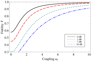
Figure 2: (Color online) The fidelity of the gate operation vs the coupling strength $\kappa_{0}$ for different squeezing of the input light. The solid line denotes the coherent input.

where we have put $\kappa=1$. Corresponding to this expression, in Fig. 2, we are able to show the fidelity of the gate operation in its dependence on the coupling strength $\kappa_{0}$ for different squeezing of the input light (in dB). As can be seen from the figure that large coupling strength are required for the achievement of high fidelities.

III noise effects and experimental feasibility

III.1 Noise effects

So far, we have neglected the noise effects. As in reality, atoms are usually contained in glass cells. Therefore, light reflections by the cell walls become inevitable. Such reflections, however, can be modeled by a beam splitter type admixture of vacuum components Fiurášek et al. (2006); Hammerer et al. (2005), which transforms the input light quadrature as $\hat{\vartheta}^{in}\to\hat{\vartheta}^{in^{\prime}}=\sqrt{1-r}\hat{\vartheta}^{in}+\sqrt{r}\hat{\vartheta}^{v}$ with $\hat{\vartheta}\in\{\hat{x}_{L,M},\hat{p}_{L,M}\}$, where $r$ is the reflection coefficient and $\hat{\vartheta}^{v}$ is the vacuum noise quadrature. On the other hand, due to the weak excitation by the light beams, the atoms also undergo dissipation. We assume that the spontaneous emission happens at a rate of $\eta/T$ Muschik et al. (2006). With these modeling, the evolution equations (4)$-$(9) are then changed into

$${\partial_{t}}{{\hat{x}}_{a}}\left(t\right)=\tilde{\kappa}^{\prime}\hat{p}_{L}^{in}\left(t\right)-\frac{\eta}{{2T}}{{\hat{x}}_{a}}\left(t\right)+\sqrt{\frac{\eta}{T}}\hat{x}_{a}^{v}\left(t\right),\\$$

$${\partial_{t}}{{\hat{p}}_{a}}\left(t\right)=-\tilde{\kappa}^{\prime}\hat{p}_{M}^{in}\left(t\right)-\frac{\eta}{{2T}}{{\hat{p}}_{a}}\left(t\right)+\sqrt{\frac{\eta}{T}}\hat{p}_{a}^{v}\left(t\right),\\$$

$$\hat{x}_{L}^{out1}\left(t\right)=\hat{x}_{L}^{in^{\prime}}\left(t\right)+\tilde{\kappa}^{\prime}{{\hat{p}}_{a}}\left(t\right),\\$$

$$\hat{p}_{L}^{out1}\left(t\right)=\hat{p}_{L}^{in^{\prime}}\left(t\right),\\$$

$$\hat{x}_{M}^{out1}\left(t\right)=\hat{x}_{M}^{in^{\prime}}\left(t\right)+\tilde{\kappa}^{\prime}{{\hat{x}}_{a}}\left(t\right),\\$$

$$\hat{p}_{M}^{out1}\left(t\right)=\hat{p}_{M}^{in^{\prime}}\left(t\right),$$ (21)

where $\hat{x}_{a}^{v}$ and $\hat{p}_{a}^{v}$ are Langevin noise operators with zero mean, having $\langle\hat{x}_{a}^{v}(t)\hat{p}_{a}^{v}(t^{\prime})\rangle=\delta(t-t^{\prime})/2$. Here, we have defined the reduced coupling strength $\tilde{\kappa}^{\prime}=\sqrt{1-r}\tilde{\kappa}$. Corresponding to this set of equations, one may derive the modified input-output relations for light

$$\hat{x}_{L}^{out1} = \hat{x}_{L}^{in^{\prime}}+\kappa^{\prime}{{\hat{p}}_{a}}\left(0\right)-\frac{{{{\kappa^{\prime}}^{2}}}}{{{T^{3/2}}}}\int_{0}^{T}{dt}$$

$$\times{e^{-\frac{{\eta t}}{{2T}}}}\left({T-t}\right)\left[{\hat{p}_{M}^{in^{\prime}}\left(t\right)-\frac{\sqrt{\eta}}{{\kappa^{\prime}}}\hat{p}_{a}^{v}\left(t\right)}\right],$$

$$\hat{x}_{M}^{out1} = \hat{x}_{M}^{in^{\prime}}+\kappa^{\prime}{{\hat{x}}_{a}}\left(0\right)+\frac{{{{\kappa^{\prime}}^{2}}}}{{{T^{3/2}}}}\int_{0}^{T}{dt}$$ (22)

$$\times{e^{-\frac{{\eta t}}{{2T}}}}\left({T-t}\right)\left[{\hat{p}_{L}^{in^{\prime}}\left(t\right)+\frac{\sqrt{\eta}}{{\kappa^{\prime}}}\hat{x}_{a}^{v}\left(t\right)}\right],$$

and for atoms

$${{\hat{x}}_{a}}\left(T\right) = {e^{-\frac{\eta}{2}}}{{\hat{x}}_{a}}\left(0\right)+\frac{1}{\sqrt{T}}\int_{0}^{T}{dt}$$

$$\times{e^{-\frac{{\eta t}}{{2T}}}}\left[{\kappa^{\prime}\hat{p}_{L}^{in^{\prime}}\left(t\right)+\sqrt{\eta}\hat{x}_{a}^{v}\left(t\right)}\right],$$

$${{\hat{p}}_{a}}\left(T\right) = {e^{-\frac{\eta}{2}}}{{\hat{p}}_{a}}\left(0\right)-\frac{1}{\sqrt{T}}\int_{0}^{T}{dt}$$ (23)

$${e^{-\frac{{\eta t}}{{2T}}}}\left[{\kappa^{\prime}\hat{p}_{M}^{in^{\prime}}\left(t\right)-\sqrt{\eta}\hat{p}_{a}^{v}\left(t\right)}\right].$$

Before reflecting back into the vapor, the two light pulses will experience another two crossing of the cell wall [see Fig. 1(a)], which transfers the light states of Eqs. (22) into $\hat{x}_{i}^{out1}\to\hat{x}_{i}^{out1^{\prime}}=\sqrt{1-2r}\hat{x}_{i}^{out1}+\sqrt{2r}\hat{x}_{i}^{v}$ with $i\in\{L,M\}$. Using the light state $\hat{x}_{i}^{out1^{\prime}}$ and the atomic state of Eqs. (23) as the input states, the second interaction occurs, resulting in the final output states

$$\hat{x}_{L}^{out2} = \sqrt{1-3r}\left[{\hat{x}_{L}^{in}+\epsilon_{1}^{-}{\kappa^{2}}\hat{p}_{M}^{in}}\right.$$

$$\left.{+\epsilon_{2}^{-}{\kappa^{2}}\hat{\tilde{p}}_{M}^{in}+\frac{\eta}{2}\kappa{{\hat{p}}_{a}}\left(0\right)}\right]+{{\hat{f}}_{v1}},$$

$$\hat{p}_{L}^{out2} = \sqrt{1-3r}\hat{p}_{L}^{in}+\sqrt{3r}\hat{p}_{L}^{v},$$

$$x_{M}^{out2} = \sqrt{1-3r}\left[{\hat{x}_{M}^{in}+\epsilon_{1}^{+}{\kappa^{2}}\hat{p}_{L}^{in}}\right.$$

$$\left.{+\epsilon_{2}^{+}{\kappa^{2}}\hat{\tilde{p}}_{L}^{in}+2\kappa\left({1-\frac{\eta}{4}}\right){{\hat{x}}_{a}}\left(0\right)}\right]+{{\hat{f}}_{v2}},$$

$$\hat{p}_{M}^{out2} = \sqrt{1-3r}\hat{p}_{M}^{in}+\sqrt{3r}\hat{p}_{M}^{v},$$ (24)

Figure 3: (Color online) (a) Gate operation fidelity $F$ vs coupling $\kappa_{0}$ in the presence of atomic decay and light reflection. The input light states are assumed to be polarization squeezed with the degree of $5$ dB. (b) Optimized fidelity vs decay rate $\eta$ for different reflection coefficient. The inset shows how the optimal coupling $\kappa_{0}$ varies with $\eta$.

where $\epsilon_{1}^{\pm}=(1-r)(1\pm 2r)({1-\frac{\eta}{2}\mp\frac{{2r}}{{1\pm 2r}}})$ and $\epsilon_{2}^{\pm}=(1-r)\frac{{(1\pm 2r)}}{{\sqrt{3}}}({\frac{\eta}{2}\pm\frac{{2r}}{{1\pm 2r}}})$, and we defined the total vacuum noise $\hat{f}_{v1}$ and $\hat{f}_{v2}$, which are a function of the vacuum operators $\hat{x}_{i}^{v}$ and $\hat{p}_{i}^{v}$, with $i\in\{a,L,M\}$. Here, $\hat{\tilde{p}}_{L,M}$ are new defined collective light modes with a temporal mode function $f(t)=(1-2t/T)$, satisfying $[\hat{\tilde{x}}_{j},\hat{\tilde{p}}_{j}]=i$ with $j\in\{L,M\}$. It is easily checked that they are independent from all other modes Hammerer et al. (2005). Unlike the ideal case, Eqs. (III.1) show that, besides the atomic position quadrature, the momentum quadrature $\hat{p}_{a}(0)$ now also appears. This term arising because of the decoherence of atoms, as we shall see, will lead to the optimal implementation of the scheme. Finally, after taking the end reflection losses into account (because of the fourth crossing of a cell wall) by damping Eqs. (III.1) with a factor $\sqrt{1-r}$ and adding appropriate noise terms, the covariance matrix of the final output state (and, thus, the fidelity) can then be calculated directly. Putting $\kappa=1$, the fidelity versus coupling strength $\kappa_{0}$ for squeezed input light with $s=\frac{1}{4}\text{ln}~{}10$ (corresponding to $5$ dB) in the presence of noises is depicted in Fig. 3(a) for parameters $r=\eta=0.01$, $r=\eta=0.05$, and $r=\eta=0.1$. In each case, there exist an optimal fidelity, $F=0.89$, $F=0.66$, and $F=0.54$, for $\kappa_{0}=19.90$, $\kappa_{0}=8.78$, and $\kappa_{0}=6.12$, respectively. As illustrated by the graph, decay and reflections losses have a significant effect on the quality of the gate operation. Losses of the latter kind, however, can be greatly reduced down (to about $0.5\%$) with improved antireflection coating Hammerer et al. (2006). Figure 3(b) shows the $\kappa_{0}$-optimized fidelity versus $\eta$ for different (small) values of the reflection parameter $r$. For $\eta=0.1$ (corresponding to the experimental conditions of Sherson et al. (2006)) and $r=0.005$, a fidelity $F=0.71$ would be possible corresponding to $\kappa_{0}=6.05$.

III.2 Experimental feasibility

To successfully and efficiently implement the $C_{Z}$ gate, it is required that (i) $T<T_{DL}$, where $T_{DL}$ represents a time in which the two beams pass through the delay lines, (ii) the coupling strength $\kappa=1$, and (iii) large interaction strength $\kappa_{0}$ is achievable. Conditions (i), as analyzed in Ref. Takano et al. (2008), is feasible within presently established techniques, i.e. by using a 1 $\mu s$ delay line Jeffrey et al. and a sub-$\mu s$ pulse Takeuchi et al. (2006). Condition (ii) has been realized in many physical systems, e.g. room temperature atomic vapors Julsgaard et al. (2004). Condition (iii), however, is by now still experimental challenge. Although, theoretically, one can always enhance the coupling strength by increasing the intensity of the light beams, or, the density of atoms, such enhancement, on the other hand, will cause high decay rate, and thus will lower the efficiency of current scheme. To overcome this limitation, we propose to inject squeezed light instead of coherent light during the spin squeezing process, which transfers the input quadratures $(\hat{x}_{ph}^{in},\hat{p}_{ph}^{in})$ into $(e^{-s}x_{ph}^{in},e^{s}\hat{p}_{ph}^{in})$. With this setting, the spin state of Eqs. (2) is then changed into

$$\hat{x}_{a}^{out}=\sqrt{1+e^{2s}\kappa_{0}^{2}}\hat{x}_{a}^{in},~{}\hat{p}_{a}^{out}=\frac{1}{\sqrt{1+e^{2s}\kappa_{0}^{2}}}\hat{p}_{a}^{in}.$$ (25)

Note that the coupling strength is now enhanced by a factor $e^{s}$. We can define the effective coupling strength $\kappa^{eff}_{0}=e^{s}\kappa_{0}$. As a result, the higher the degree of squeezing is, the larger the effective coupling strength becomes. For room temperature atomic vapors, the feasible value of coupling strength is around $\kappa_{0}\approx 1.4$ Sherson (2006). In this case, if we inject a light with $8.5$ dB of squeezing, a large coupling strength $\kappa^{eff}_{0}\approx 10$ can then be achieved.

IV conclusions

In conclusion, we have presented a simple and realistic scheme for realizing CV $C_{Z}$ gate in an atomic ensemble. The process is based on off-resonant interaction between light and spin-polarized atomic ensembles. By sending two off-resonant pulses propagating in two orthogonal directions twice through an atomic ensemble which is initially prepared in spin squeezed state, we find that a $C_{Z}$ operation between the two pulses is performed. The more the amount of spin squeezing input, the higher the fidelity we will obtain. We also considered the influences of the noise effects including the atomic decay and photon reflections by the cell walls, showing that they have a strong effect on the fidelity. Noises of later kind, however, can be greatly suppressed by adding antireflection coating to cell walls. Such suppressions enable us to achieve quite high fidelities with current experimental parameters. It is well known that offline squeezing and $C_{Z}$ gate together enable the construction of arbitrarily large CV cluster states Gu et al. (2009); Menicucci et al. (2010). Recently, offline squeezing based on atomic ensembles has been proposed by Sherson et al. Sherson and Mølmer (2006). Therefore, our proposal paves the way for the implementation of CV one-way QC based only on atomic ensembles.