Determination of electromagnetic medium from the Fresnel surface

Abstract.

We study Maxwell’s equations on a $4$-manifold where the electromagnetic medium is described by an antisymmetric $2\choose 2$-tensor $\kappa$. In this setting, the Tamm-Rubilar tensor density determines a polynomial surface of fourth order in each cotangent space. This surface is called the Fresnel surface and acts as a generalisation of the light-cone determined by a Lorentz metric; the Fresnel surface parameterises electromagnetic wave-speed as a function of direction. Favaro and Bergamin have recently proven that if $\kappa$ has only a principal part and if the Fresnel surface of $\kappa$ coincides with the light cone for a Lorentz metric $g$, then $\kappa$ is proportional to the Hodge star operator of $g$. That is, under additional assumptions, the Fresnel surface of $\kappa$ determines the conformal class of $\kappa$. The purpose of this paper is twofold. First, we provide a new proof of this result using Gröbner bases. Second, we describe a number of cases where the Fresnel surface does not determine the conformal class of the original $2\choose 2$-tensor $\kappa$. For example, if $\kappa$ is invertible we show that $\kappa$ and $\kappa^{-1}$ have the same Fresnel surfaces.

1. Introduction

The purpose of this work is to study properties of propagating electromagnetic fields in linear medium. We will work in a relativistic setting where Maxwell’s equations are written on a $4$-manifold and the electromagnetic medium is represented by an antisymmetric $2\choose 2$-tensor $\kappa$. Pointwise, such medium is determined by $36$ parameters. To understand the propagation of an electromagnetic wave in this setting, the key object is the Fresnel surface, which can be seen a generalisation of the light-cone [Rub02, HO03, PSW09]. For a Lorentz metric, the light-cone is always a polynomial surface of second order in each cotangent space. The Fresnel surface, in turn, is a polynomial surface of fourth order. For example, the Fresnel surface can be the union of two light-cones. This allows the Fresnel surface to model propagation also in birefringent medium. That is, in medium where differently polarised electromagnetic waves can propagate with different wave speeds.

The Fresnel surface is determined by the Tamm-Rubilar tensor density which is a symmetric $4\choose 0$-tensor density, which, in turn, is determined by the medium $2\choose 2$-tensor $\kappa$. This dependence is illustrated in the diagram below:

$$\quad\mbox{Medium}\,\,\kappa\quad\to\quad\mbox{Tamm-Rubilar tensor density}\quad\to\quad\mbox{Fresnel surface}.$$

In Lorentz geometry, we know the the light cone of a Lorentz metric $g$ uniquely determine $g$ up to a conformal factor [Ehr91]. In this work we will study the analogue relation between a general electromagnetic medium tensor $\kappa$ and its Fresnel surface; Can one reconstruct an electromagnetic medium from its Fresnel surface? In general, a unique reconstruction is not possible. For example, the Fresnel surface is invariant under a conformal change in the medium. Hence the Fresnel surface can, at best, determine $\kappa$ up to a conformal factor. One would then like to understand the following question:

Question 1.1.

Under what assumptions does the Fresnel surface at a point $p\in N$ determine the electromagnetic medium $\kappa|_{p}$ up to a conformal factor?

In terms of physics, Question 1.1 asks when we can reconstruct $\kappa|_{p}$ (up to a conformal factor) using only wavespeed information about the medium at $p$. A proper understanding of this question is not only of theoretical interest, but also of interest in engineering applications like electromagnetic tomography. Question 1.1 is also similar is spirit to a question in general relativity, where one would like to understand when the the conformal class of a Lorentz metric can be determined by the five dimensional manifold of null-geodesics [Low05].

Favaro and Bergamin have recently proven the following result of positive nature [FB11]: If $\kappa$ has only a principal part and if the Fresnel surface of $\kappa$ coincides with the light cone for a Lorentz metric $g$, then $\kappa$ is proportional to the Hodge star operator of $g$. That is, in a restricted class of medium, the Fresnel surface of $\kappa$ determines the conformal class of $\kappa$. An important corollary is the following: If $\kappa$ has only a principal part and its Fresnel surface coincides with the light cone for a Lorentz metric, then $\kappa$ satisfies the closure condition $\kappa^{2}=-f\operatorname{Id}$ for a function $f\colon N\to(0,\infty)$. This resolves a conjecture on whether the closure condition characterises non-birefringent medium in skewon-free medium [OFR00, HO03]. That the closure condition is sufficient, was already proven in [OH99, OFR00], but before [FB11] sufficiency was only known under additional assumptions; a proof assuming that ${\mathscr{C}}=0$ (see Section 2.4 for the definition of ${\mathscr{C}}$ in terms on $\kappa$) is given in [OFR00], and a proof in a special class of non-linear medium is given in [OR02]. For additional positive results to Question 1.1, see [LH04, Iti05, SWW10, FB11].

The main contribution of this paper is twofold. First, we give a new proof of the result quoted above from [FB11]. This is formulated as implication (iii) $\Rightarrow$ (ii) in Theorem 4.1. While the original proof in [FB11] relies on the classification of skewon-free $2\choose 2$-tensors into 23 normal forms by Schuller, Witte, and Wohlfarth [SWW10], we will use Gröbner bases to prove Theorem 4.1. Essentially, Gröbner bases is a computer algebra technique for simplifying a system polynomial equations without changing the solution set. See Appendix A.

The second contribution of this paper is given in Section 5 which contains a number of cases, where the Fresnel surface does not determine $\kappa$. In Theorem 5.1 (iv) we show that if $\kappa$ is invertible, then $\kappa$ and $\kappa^{-1}$ have the same Fresnel surfaces. Also, in Example 5.3 we construct a $\kappa$ with complex coefficients on $\mathbb{R}^{4}$. At each $p\in\mathbb{R}^{4}$, this medium is determined by one arbitrary complex number, and hence the medium can depend on both time and space. However, at each point, the Fresnel surface of $\kappa$ coincides with the usual light cone of the flat Minkowski metric $g=\operatorname{diag}(-1,1,1,1)$.

The paper is organised as follows. In Section 2 we review Maxwell’s equations and linear electromagnetic medium on a $4$-manifold. In Section 3 we describe how the Tamm-Rubilar tensor density and Fresnel surface is related to wave propagation. To derive these objects we use the approach of geometric optics. As described in Section 3, this can be seen as a step towards a relativistic theory of electromagnetic Gaussian beams (if such a theory exists). In general, Gaussian beams is an asymptotic technique for studying propagation of waves in hyperbolic systems. These solutions behave as wave packets; at each time instant, the entire energy of the solution is concentrated around one point in space. When time moves forward, the beam propagates along a curve, but always retains its shape of a Gaussian bell curve. Electromagnetic Gaussian beams are also known as quasi-photons [Kac02, Kac04, Kac05, Dah06]. For the wave equation, see [Ral82, KKL01]. For the history of Gaussian beams, see [Ral82, Pop02]. In Section 4 we prove the main result Theorem 4.1, and in Section 5 we describe a number of cases where Question 1.1 has a negative answer.

This paper relies on a number of computations done with computer algebra. Further information about these can be found on the author’s homepage.

2. Maxwell’s equations

By a manifold $M$ we mean a second countable topological Hausdorff space that is locally homeomorphic to $\mathbb{R}^{n}$ with $C^{\infty}$-smooth transition maps. All objects are assumed to be smooth where defined. Let $TM$ and $T^{\ast}M$ be the tangent and cotangent bundles, respectively, and for $k\geq 1$, let $\Lambda^{k}(M)$ be the set of $p$-covectors, so that $\Lambda^{1}(N)=T^{\ast}N$. Let $\Omega^{k}_{l}(M)$ be $k\choose l$-tensors that are antisymmetric in their $k$ upper indices and $l$ lower indices. In particular, let $\Omega^{k}(M)$ be the set of $k$-forms. Let also ${\mathfrak{X}}(M)$ be the set of vector fields, and let $C^{\infty}(M)$ be the set of functions. By $\Omega^{k}(M)\times\mathbb{R}$ we denote the set of $k$-forms that depend smoothly on a parameter $t\in\mathbb{R}$. By $T(M,\mathbb{C})$, $T^{\ast}(M,\mathbb{C})$, $\Lambda^{p}(M,\mathbb{C})$, $\Omega^{k}_{l}(M,\mathbb{C})$ and ${\mathfrak{X}}(M,\mathbb{C})$ we denote the complexification of the above spaces where component may also take complex values. Smooth complex valued functions are denoted by $C^{\infty}(M,\mathbb{C})$. The Einstein summing convention is used throughout. When writing tensors in local coordinates we assume that the components satisfy the same symmetries as the tensor.

We will use differential forms to write Maxwell’s equations. On a $3$-manifold $M$, Maxwell equations then read [BH96, HO03]

(1) $$dE = -\frac{\partial B}{\partial t},$$

(2) $$dH = \frac{\partial D}{\partial t}+J,$$

(3) $$dD = \rho,$$

(4) $$dB = 0,$$

for field quantities $E,H\in\Omega^{1}(M)\times\mathbb{R}$, $D,B\in\Omega^{2}(M)\times\mathbb{R}$ and sources $J\in\Omega^{2}(M)\times\mathbb{R}$ and $\rho\in\Omega^{3}(M)\times\mathbb{R}$. Let us emphasise that equations (1)–(4) are completely differential-topological and do not depend on any additional structure. (To be precise, the exterior derivative does depend on the smooth structure of $M$. However, for a manifold $M$ of dimension $1,2,3$ one can show that all smooth structures for $M$ are diffeomorphic. For higher dimensions the analogue result is not true. Even for $\mathbb{R}^{4}$ there are uncountably many non-diffeomorphic smooth structures [Sco05, p. 255].)

2.1. Maxwell’s equations on a $4$-manifold

Suppose $E,D,B,H$ are time dependent forms $E,H\in\Omega^{1}(M)\times\mathbb{R}$ and $D,B\in\Omega^{2}(M)\times\mathbb{R}$ and $N$ is the $4$-manifold $N=\mathbb{R}\times M$. Then we can define forms $F,G\in\Omega^{2}(N)$ and $j\in\Omega^{3}(N)$,

(5) $$F = B+E\wedge dt,$$

(6) $$G = D-H\wedge dt,$$

(7) $$j = \rho-J\wedge dt.$$

Now fields $E,D,B,H$ solve Maxwell’s equations equations (1)–(4) if and only if

(8) $$dF = 0,$$

(9) $$dG = j,$$

where $d$ is the exterior derivative on $N$. More generally, if $N$ is a $4$-manifold and $F,G,j$ are forms $F,G\in\Omega^{2}(N)$ and $j\in\Omega^{3}(N)$ we say that $F,G$ solve Maxwell’s equations (for a source $j$) when equations (8)–(9) hold. By an electromagnetic medium on $N$ we mean a map

$$\kappa\colon\Omega^{2}(N) \to \Omega^{2}(N).$$

We then say that $2$-forms $F,G\in\Omega^{2}(N)$ solve Maxwell’s equations in medium $\kappa$ if $F$ and $G$ satisfy equations (8)–(9) and

(10) $$G = \kappa(F).$$

Equation (10) is known as the constitutive equation. If $\kappa$ is invertible, it follows that one can eliminate half of the free variables in Maxwell’s equations (8)–(9). We assume that $\kappa$ is linear and local so that we can represent $\kappa$ by an antisymmetric $2\choose 2$-tensor $\kappa\in\Omega^{2}_{2}(N)$. If in coordinates $\{x^{i}\}_{i=0}^{3}$ for $N$ we have

(11) $$\kappa = \frac{1}{2}\kappa^{ij}_{lm}dx^{l}\otimes dx^{m}\otimes\frac{\partial}{\partial x^{i}}\otimes\frac{\partial}{\partial x^{j}}$$

and $F=F_{ij}dx^{i}\otimes dx^{j}$ and $G=G_{ij}dx^{i}\otimes dx^{j}$, then constitutive equation (10) reads

(12) $$G_{ij} = \frac{1}{2}\kappa_{ij}^{rs}F_{rs}.$$

2.2. Decomposition of electromagnetic medium

Let $N$ be a $4$-manifold. Then at each point on $N$, a general antisymmetric $2\choose 2$-tensor depends on $36$ parameters. Such tensors canonically decompose into three linear subspaces. The motivation for this decomposition is that different components in the decomposition enter in different parts of electromagnetics. See [HO03, Section D.1.3]. The below formulation is taken from [Dah09].

If $\kappa\in\Omega^{2}_{2}(N)$ we define the trace of $\kappa$ as the smooth function $N\to\mathbb{R}$ given by

$$\operatorname{trace}\kappa = \frac{1}{2}\kappa_{ij}^{ij}$$

when $\kappa$ is locally given by equation (11). Writing $\operatorname{Id}$ as in equation (11) gives $\operatorname{Id}^{ij}_{rs}=\delta^{i}_{r}\delta^{j}_{s}-\delta^{i}_{s}\delta^{j}_{r}$, so $\operatorname{trace}\operatorname{Id}=6$ when $\dim N=4$.

Proposition 2.1 (Decomposition of a $2\choose 2$-tensors).

Let $N$ be a $4$-manifold, and let

$$Z = \{\kappa\in\Omega^{2}_{2}(N):u\wedge\kappa(v)=\kappa(u)\wedge v\,\,\mbox{for all}\,\,u,v\in\Omega^{2}(N),$$

$$\quad\quad\quad\quad\quad\quad\operatorname{trace}\kappa=0\},$$

$$W = \{\kappa\in\Omega^{2}_{2}(N):u\wedge\kappa(v)=-\kappa(u)\wedge v\,\,\mbox{for all}\,\,u,v\in\Omega^{2}(N)\}$$

$$= \{\kappa\in\Omega^{2}_{2}(N):u\wedge\kappa(v)=-\kappa(u)\wedge v\,\,\mbox{for all}\,\,u,v\in\Omega^{2}(N),$$

$$\quad\quad\quad\quad\quad\quad\operatorname{trace}\kappa=0\},$$

$$U = \{f\operatorname{Id}\in\Omega^{2}_{2}(N):f\in C^{\infty}(N)\}.$$

Then

(13) $$\Omega^{2}_{2}(N) = Z\,\,\oplus\,\,W\,\,\oplus\,\,U,$$

and pointwise, $\dim Z=20$, $\dim W=15$ and $\dim U=1$.

If we write a $\kappa\in\Omega^{2}_{2}(N)$ as

$$\kappa = {}^{(1)}\!\kappa\,\,+\,\,^{(2)}\!\kappa\,\,+\,\,^{(3)}\!\kappa$$

with ${}^{(1)}\!\kappa\in Z$, ${}^{(2)}\!\kappa\in W$, ${}^{(3)}\!\kappa\in U$, then we say that ${}^{(1)}\!\kappa$ is the principal part, ${}^{(2)}\!\kappa$ is the skewon part, ${}^{(3)}\!\kappa$ is the axion part of $\kappa$.

2.3. The Hodge star operator

By a pseudo-Riemann metric on a manifold $M$ we mean a symmetric real $0\choose 2$-tensor $g$ that is non-degenerate. If $M$ is not connected we also assume that $g$ has constant signature. If $g$ is positive definite, we say that $g$ is a Riemann metric. By $\sharp$ and $\flat$ we denote the isomorphisms $\sharp\colon T^{\ast}M\to TM$ and $\flat\colon TM\to T^{\ast}M$. By $\mathbb{R}$-linearity we extend $g$, $\sharp$ and $\flat$ to complex arguments. Moreover, we extend $g$ also to covectors by setting $g(\xi,\eta)=g(\xi^{\sharp},\eta^{\sharp})$ when $\xi,\eta\in\Lambda^{1}_{p}(N,\mathbb{C})$.

Suppose $g$ is a pseudo-Riemann metric on a orientable manifold $M$ with $n=\dim M\geq 2$. For $p\in\{0,\ldots,n\}$, the Hodge star operator $\ast$ is the map $\ast\colon\Omega^{p}(M)\to\Omega^{n-p}(M)$ defined as [AMR88, p. 413]

$$\ast(dx^{i_{1}}\wedge\cdots\wedge dx^{i_{p}}) = \frac{\sqrt{|\det g|}}{(n-p)!}g^{i_{1}l_{1}}\cdots g^{i_{p}l_{p}}\varepsilon_{l_{1}\cdots l_{p}\,l_{p+1}\cdots l_{n}}dx^{l_{p+1}}\wedge\cdots\wedge dx^{l_{n}},$$

where $x^{i}$ are local coordinates in an oriented atlas, $g=g_{ij}dx^{i}\otimes dx^{j}$, $\det g=\det g_{ij}$, $g^{ij}$ is the $ij$th entry of $(g_{ij})^{-1}$, and $\varepsilon_{l_{1}\cdots l_{n}}$ is the Levi-Civita permutation symbol. We treat $\varepsilon_{l_{1}\cdots l_{n}}$ as a purely combinatorial object (and not as a tensor density). We also define $\varepsilon^{l_{1}\cdots l_{n}}=\varepsilon_{l_{1}\cdots l_{n}}$.

If $g$ is a pseudo-Riemann metric on an oriented $4$-manifold $N$, then the Hodge star operator for $g$ induces a $2\choose 2$-tensor $\kappa=\ast_{g}\in\Omega^{2}_{2}(N)$. If $\kappa$ is written as in equation (11) for local coordinates $x^{i}$ then

(14) $$\kappa^{ij}_{rs} = \sqrt{|g|}g^{ia}g^{jb}\varepsilon_{abrs}.$$

Proposition 2.2.

Suppose $g$ is a pseudo-Riemann metric on an orientable $4$-manifold $N$. Then $\ast_{g}$ defines a $2\choose 2$-tensor with only a principal part.

Proof.

Let $\kappa$ be the $2\choose 2$-tensor induced by $\ast_{g}$. Then $u\wedge\kappa(v)=\kappa(u)\wedge v$ for all $u,v\in\Omega^{2}(N)$ [AMR88, p. 412]. By Theorem 2.1 it therefore suffices to prove that $\operatorname{trace}\kappa=0$. Let us fix $p\in N$ and let $x^{i}$ are local coordinates for $N$ such that $g|_{p}$ is diagonal. If $\kappa$ is written as in equation (11) then equation (14) implies that $\operatorname{trace}\kappa=\frac{1}{2}\kappa^{ij}_{ij}=0$ since $g^{ij}$ is diagonal and $\varepsilon_{ijkl}$ is non-zero only when $ijkl$ are distinct. ∎

A pseudo-Riemann metric $g$ is a Lorentz metric if $M$ is $4$-dimensional and $g$ has signature $(+---)$ or $(-+++)$. For a Lorentz metric, we define the null cone at $p$ as the set $\{\xi\in\Lambda^{1}_{p}(M,\mathbb{R}):g(\xi,\xi)=0\}.$ Usually, the null cone is defined as a subset in the tangent bundle. The motivation for treating the null-cone in the cotangent bundle is given by equation (3.6).

The next theorem shows that the conformal class of a Lorentz metric $g$ can be represented either using the $2\choose 2$-tensor $\ast_{g}$ or the null cone of $g$.

Theorem 2.3.

Suppose $g,h$ are Lorentz metrics on an orientable $4$-manifold $N$. Then the following are equivalent:

1. There exists a non-vanishing function $\lambda\in C^{\infty}(N)$ such that $h=\lambda g$.

2. $\ast_{g}=\ast_{h}$, where $\ast_{g}$ and $\ast_{h}$ are the $2\choose 2$-tensors defined by $g$ and $h$, respectively.

3. $g$ and $h$ have the same null cones.

Proof.

Implications (i) $\Rightarrow$ (ii) and (i) $\Rightarrow$ (iii) are clear. Implication (ii) $\Rightarrow$ (i) is proven in [DKS89, Theorem 1], and implication (iii) $\Rightarrow$ (i) is proven in [Ehr91, Theorem 3]. See also [MS08]. ∎

2.4. Decomposition of $\kappa$ into four $3\times 3$ matrices

Suppose $(x^{0},x^{1},x^{2},x^{3})$ are local coordinates for $N=\mathbb{R}\times M$ such that $x^{0}$ is the coordinate for $\mathbb{R}$ and $(x^{1},x^{2},x^{3})$ are coordinates for $M$. If forms $F,G$ are given by equations (5)–(6), then

$$F_{i0}=E_{i},\quad F_{ij}=B_{ij},\quad G_{i0}=-H_{i},\quad G_{ij}=D_{ij}$$

for all $i,j=1,2,3$ and equation (12) then reads

(15) $$H_{i} = -\kappa_{i0}^{r0}E_{r}-\frac{1}{2}\kappa_{i0}^{rs}B_{rs},$$

(16) $$D_{ij} = \kappa_{ij}^{r0}E_{r}+\frac{1}{2}\kappa_{ij}^{rs}B_{rs},$$

where $i,j=1,2,3$ and $r,s$ are summed over $1,2,3$.

Next we show that in coordinates $(x^{0},x^{1},x^{2},x^{3})$ the tensor $\kappa$ is represented by four $3\times 3$-matrices. To do this, let $\ast$ is the Hodge star operator induced by the Euclidean metric on $x^{1},x^{2},x^{3}$ so that $\ast dx^{i}=\frac{1}{2}\sum_{a,b=1}^{3}\varepsilon^{iab}dx^{a}\wedge dx^{b}$. Thus $B=\sum_{i=1}^{3}B^{i}\ast\!dx^{i}$ where $B^{i}=\frac{1}{2}\varepsilon^{ijk}B_{jk}$ and $B_{mn}=\varepsilon_{imn}B^{i}$. In the same way we define $D^{1},D^{2},D^{3}$. Now components $D^{i}$ and $B^{i}$ represent $2$-forms $D$ and $B$ in the basis $\{\ast dx^{i}\}_{i=1}^{3}$, and by equations (15)–(16),

(17) $$H_{i} = {\mathscr{C}}^{r}\,_{i}(-E_{r})+{\mathscr{B}}_{ri}B^{r},$$

(18) $$D^{i} = {\mathscr{A}}^{ri}(-E_{r})+{\mathscr{D}}_{r}\,^{i}B^{r},$$

where $i\in\{1,2,3\}$, $r$ is summed over $1,2,3$, and

$${\mathscr{C}}^{r}\,_{i}=\kappa^{r0}_{i0},\quad{\mathscr{B}}_{ri}=-\frac{1}{2}\varepsilon_{rab}\kappa^{ab}_{i0},\quad{\mathscr{A}}^{ri}=-\frac{1}{2}\varepsilon^{iab}\kappa^{r0}_{ab},\quad{\mathscr{D}}_{r}\,\!^{i}=\frac{1}{4}\varepsilon_{rmn}\varepsilon^{iab}\kappa^{mn}_{ab}.$$

Here $r$ index rows and $i$ index columns in $3\times 3$ matrices ${\mathscr{A}},{\mathscr{B}},{\mathscr{C}},{\mathscr{D}}$. Inverting the relations gives

$$\kappa^{0r}_{0i}={\mathscr{C}}^{r}\,\!_{i},\quad\kappa^{ij}_{0r}=\varepsilon^{kij}{\mathscr{B}}_{kr},\quad\kappa^{0i}_{rs}=\varepsilon_{krs}{\mathscr{A}}^{ik},\quad\kappa^{ij}_{rs}=\varepsilon_{krs}\varepsilon^{lij}{\mathscr{D}}_{l}\,\!^{k},$$

where $i,j,r,s\in\{1,2,3\}$ and $k,l$ are summed over $1,2,3$.

The above matrices ${\mathscr{A}},{\mathscr{B}},{\mathscr{C}},{\mathscr{D}}$ coincide with the matrices ${\mathscr{A}},{\mathscr{B}},{\mathscr{C}},{\mathscr{D}}$ defined in [HO03, Section D.1.6] and [Rub02]. Since these matrices are only part of tensor $\kappa$, they do not transform in a simple way under a general coordinate transformation in $N$ (see equations D.5.28–D.5.30 in [HO03]). However, if $\{x^{i}\}_{i=0}^{3}$ and $\{\widetilde{x}^{i}\}_{i=0}^{3}$ are overlapping coordinates such that

$$\widetilde{x}^{0} = x^{0},$$

$$\widetilde{x}^{i} = \widetilde{x}^{i}(x^{1},x^{2},x^{3}),\quad i\in\{1,2,3\}.$$

Then we have transformation rules

(19) $$\widetilde{\mathscr{C}}^{r}\,_{i} = {\mathscr{C}}^{a}\,_{b}\frac{\partial x^{b}}{\partial\widetilde{x}^{i}}\frac{\partial\widetilde{x}^{r}}{\partial x^{a}},$$

(20) $$\widetilde{\mathscr{B}}_{ri} = \det\left(\frac{\partial\widetilde{x}^{m}}{\partial x^{n}}\right){\mathscr{B}}_{ab}\frac{\partial x^{a}}{\partial\widetilde{x}^{r}}\frac{\partial x^{b}}{\partial\widetilde{x}^{i}},$$

(21) $${\widetilde{\mathscr{A}}}^{ri} = \det\left(\frac{\partial x^{m}}{\partial\widetilde{x}^{n}}\right){\mathscr{A}}^{ab}\frac{\partial\widetilde{x}^{r}}{\partial x^{a}}\frac{\partial\widetilde{x}^{i}}{\partial x^{b}},$$

(22) $$\widetilde{\mathscr{D}}_{r}\,\!^{i} = {\mathscr{D}}_{a}\,\!^{b}\frac{\partial\widetilde{x}^{i}}{\partial x^{b}}\frac{\partial x^{a}}{\partial\widetilde{x}^{r}}.$$

If ${}^{(2)}\!\kappa=0$ then Proposition 2.1 implies that $\kappa$ is pointwise determined by $21$ coefficients. The next proposition shows that these coefficients can pointwise be reduced to $18$ when the coordinates are chosen suitably.

Proposition 2.4.

Suppose $N$ is a $4$-manifold and $\kappa\in\Omega^{2}_{2}(N)$. Then

1. $\kappa$ has no skewon component if and only if locally

   $${\mathscr{A}}={\mathscr{A}}^{T},\quad{\mathscr{B}}={\mathscr{B}}^{T},\quad{\mathscr{C}}={\mathscr{D}}^{T},$$

   where ^T is the matrix transpose, and ${\mathscr{A}},{\mathscr{B}},{\mathscr{C}},{\mathscr{D}}$ are defined as above.

2. Let $p\in N$. If $\kappa$ has no skewon component, then there are local coordinates around $p$ such that ${\mathscr{A}}$ is diagonal at $p$.

3. Let $p\in N$. If $\kappa$ has no skewon component and $g$ is a Lorentz metric on $N$ there are local coordinates around $p$ such that ${\mathscr{A}}|_{p}$ is diagonal and for some $k\in\{\pm 1\}$ we have $g|_{p}=k\operatorname{diag}(-1,1,1,1)$.

Proof.

Part (i) follows by [HO03, Equation D.1.100]. Since we can always introduce a Lorentz metric in local coordinates for $N$, part (ii) will follow from part (iii). For part (iii), let $x^{i}$ be coordinates around $p$ such that $g|_{p}=k\operatorname{diag}(-1,1,1,1)$ for $k\in\{\pm 1\}$. By (i), matrix ${\mathscr{A}}|_{p}$ is symmetric, so we can find an orthogonal $3\times 3$ matrix $P=(P^{i}\,\,_{j})_{ij}$ such that $P{\mathscr{A}}P^{T}$ is diagonal and $\det P=1$. A suitable coordinate system is given by $\widetilde{x}^{0}=x^{0}$ and $\widetilde{x}^{i}=\sum_{j=1}^{3}P^{i}\,_{j}x^{j}.$ ∎

3. Geometric optics solutions

Let $\kappa\in\Omega^{2}_{2}(N)$ on a $4$-manifold $N$, and let $F$ and $G$ be asymptotic sums

(23) $$F=\operatorname{Re}\left\{e^{iP\Phi}\sum_{k=0}^{\infty}\frac{A_{k}}{(iP)^{k}}\right\},\quad G=\operatorname{Re}\left\{e^{iP\Phi}\sum_{k=0}^{\infty}\frac{B_{k}}{(iP)^{k}}\right\},$$

where $P>0$ is a constant, $\Phi\in C^{\infty}(N,\mathbb{C})$ and $A_{k},B_{k}\in\Omega^{2}(N,\mathbb{C})$. Substituting $F$ and $G$ into the sourceless Maxwell equations and differentiating termwise shows that $F$ and $G$ form an asymptotic solution provided that

(24) $$d\Phi\wedge A_{0} = 0,$$

(25) $$d\Phi\wedge B_{0} = 0,$$

(26) $$B_{k} = \kappa A_{k},$$

(27) $$d\Phi\wedge A_{k+1}+dA_{k} = 0,$$

(28) $$d\Phi\wedge B_{k+1}+dB_{k} = 0,\quad k=0,1,\ldots.$$

In equation (26) we treat $\kappa$ as a linear map $\kappa\colon\Omega^{2}(N,\mathbb{C})\to\Omega^{2}(N,\mathbb{C})$. In equation (23) function $\Phi$ is called a phase function, and forms $A_{k},B_{k}$ are called amplitudes. We will assume that $\operatorname{Im}\Phi\geq 0$, so that $F$ and $G$ remain bounded even if we take $P\to\infty$.

Lemma 3.1.

Suppose $N$ is a smooth manifold, and let $q$ be a $1$-form $q\in\Omega^{1}(N,\mathbb{C})$ that is nowhere zero.

1. If $q\wedge A=0$ for some $A\in\Omega^{k}(N,\mathbb{C})$ where $k\geq 1$, then there exists a $(k-1)$-form $a\in\Omega^{k-1}(N,\mathbb{C})$ such that $A=q\wedge a$.

2. If $q\wedge a=q\wedge a^{\prime}$ for some $a,a^{\prime}\in\Omega^{1}(N,\mathbb{C})$, then $a=a^{\prime}+fq$ for some $f\in C^{\infty}(N,\mathbb{C})$.

Proof.

Let $\sharp$ be the isomorphism $T^{\ast}N\to TN$ induced by an auxiliary (positive definite) Riemann metric on $N$, and let $\|\cdot\|$ be the induced norms on $TN$ and $T^{\ast}N$. Let also $q=\alpha+i\beta$, where $\alpha=\operatorname{Re}q$ and $\beta=\operatorname{Im}q$. Then vector field $X\in{\mathfrak{X}}(N,\mathbb{C})$ given by

$$X = \frac{\alpha^{\sharp}-i\beta^{\sharp}}{\|\alpha\|^{2}+\|\beta\|^{2}}$$

satisfies $q(X)=1$. Contracting $q\wedge A=0$ by $X$ gives part (i). Part (ii) follows by taking $A=a-a^{\prime}$ in part (i). ∎

In this work we will only analyse the leading amplitudes $A_{0}$ and $B_{0}$. However, since $B_{0}=\kappa(A_{0})$, it suffices to study $A_{0}$ in more detail. Let us assume that $\Phi$, $A_{0}$ and $B_{0}$ solve equations (24)–(26). Then Lemma 3.1 (i) implies that there exists a $1$-form $a_{0}\in\Omega^{1}(N,\mathbb{C})$ such that $A_{0}=d\Phi\wedge a_{0},$ whence

(29) $$d\Phi\wedge\kappa(d\Phi\wedge a_{0}) = 0.$$

For $N=\mathbb{R}\times M$ where $M$ is a $3$-manifold and for special choices for $\kappa$, $\Phi$ and amplitudes $A_{k},B_{k}$, equation (23) define an electromagnetic Gaussian beam (see Section 1). In this setting, $\Phi|_{p}$ and $d\Phi|_{p}$ are both real when $p$ is at a centre of a Gaussian beam. With the above as motivation we will hereafter only study equation (29) at a point $p\in N$ where $d\Phi$ is real. From equation (23) we then see that $d\Phi|_{p}$ is the direction of most rapid oscillation (or direction of propagation) for $F$. Since $A_{0}=d\Phi\wedge a_{0}$, the $1$-form $a_{0}$, in turn, determines the polarisation of the solution in equation (23). Equation (29) is thus a condition that constrains possible polarisations once the direction of propagation is known. Since equation (29) is a linear in $a_{0}$, we may study the dimension of the the solution space for $a_{0}$. To do this, let $\xi\in\Lambda^{1}_{p}(N)$ for some $p\in N$ and for $\xi$ let $L_{\xi}$ be the linear map $L_{\xi}\colon\Lambda^{1}_{p}(N)\to\Lambda^{3}_{p}(N)$,

(30) $$L_{\xi}(\alpha) = \xi\wedge\kappa(\xi\wedge\alpha),\quad\alpha\in\Lambda_{p}^{1}(N).$$

We have $\xi\in\operatorname{ker}L_{\xi}$. For all $\xi\in\Lambda^{1}_{p}N{\setminus\{0\}}$ we can then find a (non-unique) vector subspace $V_{\xi}\subset\Lambda^{1}_{p}N$ such that

(31) $$\operatorname{ker}L_{\xi} = V_{\xi}\,\oplus\,\operatorname{span}\xi.$$

Let $\xi=d\Phi|_{p}$ be nonzero. Then $V_{\xi}{\setminus\{0\}}$ parameterises possible $a_{0}$ that solve equation (29) and for which $A_{0}=d\Phi\wedge a_{0}$ is nonzero. For a general $\kappa\in\Omega^{2}_{2}(N)$ and $\xi\in\Lambda^{1}(N){\setminus\{0\}}$ we can have $\dim V_{\xi}\in\{0,1,2,3\}$: Proposition 3.7 will show that $\dim V_{\xi}$ can be $0$ or $2$, Example 3.8 shows that $\dim V_{\xi}$ can be $1$, and the next proposition characterise $\kappa|_{p}$ when $\dim V_{\xi}=3$ for all $\xi\in\Lambda_{p}^{1}(N){\setminus\{0\}}$.

Proposition 3.2.

Let $\kappa\in\Omega^{2}_{2}(N)$ on a $4$-manifold $N$ and let $p\in N$. Then the following are equivalent:

1. $\kappa|_{p}$ is of axion type.

2. $\dim V_{\xi}=3$ for all $\xi\in\Lambda_{p}^{1}(N){\setminus\{0\}}$.

Proof.

Implication (i) $\Rightarrow$ (ii) is clear. For the converse direction suppose that (ii) holds and $x^{i}$ are local coordinates around $p$. It follows that

$$\zeta\wedge\xi\wedge\kappa(\xi\wedge\alpha) = 0,\quad\alpha,\xi,\zeta\in\Lambda^{1}_{p}(N).$$

If locally $\xi=\xi_{i}dx^{i}|_{p}$ then $\xi_{i}\xi_{j}\kappa^{ir}_{ab}\varepsilon^{jsab}=0.$ Differentiating with respect to ${\xi_{c}}$ and ${\xi_{d}}$ gives

$$\kappa^{cr}_{ab}\varepsilon^{dsab}+\kappa^{dr}_{ab}\varepsilon^{csab} = 0.$$

With computer algebra it follows that $\kappa=\frac{1}{6}\operatorname{trace}\kappa\,\,\operatorname{Id}$ and (i) follows. ∎

3.1. Fresnel surface

Let $\kappa\in\Omega^{2}_{2}(N)$ on a $4$-manifold $N$. If $\kappa$ is locally given by equation (11) in coordinates $x^{i}$, let

$${\mathscr{G}}^{ijkl}_{0} = \frac{1}{48}\kappa^{a_{1}a_{2}}_{b_{1}b_{2}}\kappa^{a_{3}i}_{b_{3}b_{4}}\kappa^{a_{4}j}_{b_{5}b_{6}}\varepsilon^{b_{1}b_{2}b_{5}k}\varepsilon^{b_{3}b_{4}b_{6}l}\varepsilon_{a_{1}a_{2}a_{3}a_{4}}.$$

In overlapping coordinates $\{\widetilde{x}^{i}\}$, these coefficients transform as

(32) $$\widetilde{\mathscr{G}}_{0}^{ijkl} = \det\left(\frac{\partial x^{r}}{\partial\widetilde{x}^{s}}\right)\,{\mathscr{G}}_{0}^{abcd}\frac{\partial\widetilde{x}^{i}}{\partial x^{a}}\frac{\partial\widetilde{x}^{j}}{\partial x^{b}}\frac{\partial\widetilde{x}^{k}}{\partial x^{c}}\frac{\partial\widetilde{x}^{l}}{\partial x^{d}}.$$

Thus components ${\mathscr{G}}^{ijkl}_{0}$ define a tensor density ${\mathscr{G}}_{0}$ on $N$ of weight $1$. The Tamm-Rubilar tensor density [Rub02, HO03] is the symmetric part of ${\mathscr{G}}_{0}$ and we denote this tensor density by ${\mathscr{G}}$. In coordinates, ${\mathscr{G}}^{ijkl}={\mathscr{G}}^{(ijkl)}_{0}$, where parenthesis indicate that indices $ijkl$ are symmetrised with scaling $1/4!$. Using tensor density ${\mathscr{G}}$, the Fresnel surface at a point $p\in N$ is defined as

(33) $$F_{p} = \{\xi\in\Lambda^{1}_{p}(N):{\mathscr{G}}^{ijkl}\xi_{i}\xi_{j}\xi_{k}\xi_{l}=0\}.$$

By equation (32), the definition of $F_{p}$ does not depend on local coordinates. Let $F$ be the disjoint union of all Fresnel surfaces, $F=\coprod_{p\in N}F_{p}$. To indicate that $F_{p}$ and $F$ depend on $\kappa$ we also write $F_{p}(\kappa)$ and $F(\kappa)$.

If $\xi\in F_{p}$ then $\lambda\xi\in F_{p}$ for all $\lambda\in\mathbb{R}$. In particular $0\in F_{p}$ for each $p\in N$. When ${\mathscr{G}}|_{p}$ is non-zero, equation (33) shows that $F_{p}$ is a fourth order surface in $\Lambda^{1}_{p}(N)$, so $F_{p}$ may contain non-smooth self intersections.

Theorem 3.3.

Suppose $N$ is a $4$-manifold and $\kappa\in\Omega^{2}_{2}(N)$. If $\xi\in\Lambda^{1}_{p}(N)$ is non-zero, then the following are equivalent:

1. $\dim V_{\xi}\geq 1$ where $V_{\xi}$ are defined as in equation (31).

2. $\xi$ belongs to the Fresnel surface $F_{p}\subset\Lambda^{1}_{p}(N)$.

Proof.

Let $\{x^{i}\}_{i=0}^{3}$ be coordinates around $p$ such that $dx^{0}|_{p}=\xi$ and let $\ast$ be the Hodge star operator induced by the Euclidean Riemann metric $g_{ij}=\delta_{ij}$ in these coordinates. Let $P\colon\Lambda_{p}^{1}(N)\to\Lambda_{p}^{1}(N)$ be the map $P=2\ast\circ L_{\xi}$. Then locally

$$P(\alpha) = \sum_{j=0}^{3}\alpha_{i}\varepsilon^{0abj}\kappa^{0i}_{ab}dx^{j},$$

where $\alpha=\alpha_{i}dx^{i}|_{p}$ and $\kappa^{ij}_{ab}$ are defined as in equation (11). It follows that in the basis $\{dx^{i}|_{p}\}_{i=0}^{3}$, the map $P$ is represented by the $4\times 4$ matrix $\operatorname{diag}(0,Q)$, where $Q$ is the $3\times 3$ matrix $Q^{ij}=\varepsilon^{0abj}\kappa^{0i}_{ab}$, $i,j\in\{1,2,3\}$. Now $\dim V_{\xi}\geq 1$ is equivalent with $\dim\operatorname{ker}P\geq 2$ which is equivalent with $\det Q=0$. Writing out $\det Q=0$ using

$$\det Q = \frac{1}{3!}\varepsilon_{abc}\varepsilon_{ijk}Q^{ai}Q^{bj}Q^{ck}$$

gives ${\mathscr{G}}^{ijkl}\xi_{i}\xi_{j}\xi_{k}\xi_{l}=0$. We omit the proof of the last step which can be found in [Rub02] and [HO03, p. 267 – 268]. ∎

Suppose $g$ is a pseudo-Riemann metric on an orientable $4$-manifold $N$ and $\kappa\in\Omega^{2}_{2}(N)$. Then $g$ and $\kappa$ define a symmetric $4\choose 0$-tensor on $N$ by

(34) $${\mathscr{G}}_{g,\kappa} = \frac{1}{\sqrt{|\operatorname{det}g|}}\,\,{\mathscr{G}}^{ijkl}\frac{\partial}{\partial x^{i}}\otimes\frac{\partial}{\partial x^{j}}\otimes\frac{\partial}{\partial x^{k}}\otimes\frac{\partial}{\partial x^{l}},$$

where ${\mathscr{G}}^{ijkl}$ are local components of the Tamm-Rubilar tensor density for $\kappa$, and $x^{i}$ are coordinates in an oriented atlas for $N$.

A key property of symmetric $p\choose 0$-tensors is that they are completely determined by their values on the diagonal [Muj06, PSW09]. For symmetric $4\choose 0$-tensors on a $4$-manifold (like ${\mathscr{G}}_{g,\kappa}$), the precise statement is contained in the following polarisation identity.

Proposition 3.4.

Suppose $L$ is a symmetric $4\choose 0$-tensor on a $4$-manifold $N$. If $x_{1},x_{2},x_{3},x_{4}\in\Lambda^{1}_{p}(N)$ then

$$L(x_{1},x_{2},x_{3},x_{4}) = \frac{1}{4!2^{4}}\sum_{\theta_{i}\in\{\pm 1\}}\theta_{1}\theta_{2}\theta_{3}\theta_{4}\,L(\sum_{i=1}^{4}\theta_{i}x_{i},\ldots,\sum_{i=1}^{4}\theta_{i}x_{i}).$$

3.2. Electromagnetic medium induced by a Hodge star operator

In Proposition 2.2 we saw that a pseudo-Riemann metric on a $4$-manifold induces a $2\choose 2$-tensor $\kappa$ with only a principal part. The next example shows how standard isotropic electromagnetic medium can be modelled using a Lorentz metric on $\mathbb{R}^{4}$.

Example 3.5.

On $N=\mathbb{R}\times\mathbb{R}^{3}$ let $\kappa$ be the $2\choose 2$-tensor determined $3\times 3$ matrices

$${\mathscr{A}}=-\epsilon\operatorname{Id},\quad{\mathscr{B}}=\mu^{-1}\operatorname{Id},\quad{\mathscr{C}}={\mathscr{D}}=0,$$

where $\epsilon,\mu\colon\mathbb{R}^{3}\to(0,\infty)$. Then constitutive equations (17)–(18) are equivalent with the isotropic constitutive equations

(35) $$D = \epsilon\ast_{0}E,$$

(36) $$B = \mu\ast_{0}H,$$

where $\epsilon$ is the permittivity and $\mu$ is the permeability of the medium and $\ast_{0}$ is the Hodge star operator induced by the Euclidean metric on $\mathbb{R}^{3}$. If $\kappa$ is the $2\choose 2$-tensor defined as $\kappa=\sqrt{\frac{\epsilon}{\mu}}\ast_{g}$ where $g$ is the Lorentz metric $g=\operatorname{diag}(-\frac{1}{\epsilon\mu},1,1,1)$, then equations (35)–(36) are equivalent with equation (10). $\Box$

The next proposition shows that if $g$ is a pseudo-Riemann metric with signature $(++++)$ or $(----)$ then the medium with $\kappa=\ast_{g}$ has no asymptotic solutions. That is, if $d\Phi|_{p}$ is non-zero, then equation (29) implies that $A_{0}|_{p}=0$. The proposition also shows that if $\kappa=\ast_{g}$ for an indefinite metric $g$, then $A_{0}$ can be non-zero only when $d\Phi|_{p}$ is a null covector, that is, when $g(d\Phi|_{p},d\Phi|_{p})=0$.

Let $\operatorname{sgn}\colon\mathbb{R}\to\{-1,+1\}$ be the sign function, $\operatorname{sgn}x=-1$ for $x<0$, $\operatorname{sgn}x=0$ for $x=0$ and $\operatorname{sgn}x=1$ for $x>0$.

Proposition 3.6.

Let $g$ and $h$ be pseudo-Riemann metrics on $N$ on an orientable $4$-manifold $N$. Then

$${\mathscr{G}}_{h,\ast g}(\xi,\xi,\xi,\xi) = \operatorname{sgn}(\det g)\,\sqrt{\frac{|\det g|}{|\det h|}}\left(g(\xi,\xi)\right)^{2},\quad\xi\in\Lambda^{1}(N).$$

Thus the Fresnel surface induced by the $2\choose 2$-tensor $\ast_{g}$ is given by

$$F(\ast_{g}) = \{\xi\in\Lambda^{1}(N):g(\xi,\xi)=0\}.$$

Proof.

Let ${\mathscr{G}}^{ijkl}$ be components for the Tamm-Rubilar tensor density for $\ast_{g}$. Computer algebra then gives

$${\mathscr{G}}^{abcd}\xi_{a}\xi_{b}\xi_{c}\xi_{d} = \operatorname{sgn}(\det g)\,\sqrt{|\det g|}\left(g(\xi,\xi)\right)^{2},$$

where $\xi=\xi_{a}dx^{a}$ and the claim follows by equation (34). ∎

We know that a general plane wave in homogeneous isotropic medium in $\mathbb{R}^{3}$ can be written as a sum of two circularly polarised plane waves with opposite handedness. The Bohren decomposition generalise this classical result to electromagnetic fields in homogeneous isotropic chiral medium [LSTV94]. The Moses decomposition, or helicity decomposition, further generalise this decomposition to arbitrary vector fields on $\mathbb{R}^{3}$. For a decomposition of Maxwell’s equations using this last decomposition, see [Mos71, Dah04]. In all of these cases, an electromagnetic wave can be polarised in two different ways. Part (i) in the next proposition shows that this is also the case for asymptotic solutions as defined above when the medium is given by the Hodge star operator of a indefinite metric.

Proposition 3.7.

Let $N$ be an orientable $4$-dimensional manifold, and let $\kappa\in\Omega^{2}_{2}(N)$ the $2\choose 2$-tensor $\kappa=\ast_{g}$ induced by a pseudo-Riemann metric $g$ on $N$.

1. If $\xi\in\Lambda^{1}(N)$ is non-zero, and $V_{\xi}$ is as in equation (31), then

   $$\dim V_{\xi} = \begin{cases}2,&\mbox{when}\,\,\xi\in F(\kappa),\\ 0,&\mbox{when}\,\,\xi\notin F(\kappa).\end{cases}$$

2. If $\xi\in F(\kappa)$ is non-zero, and $L_{\xi}$ is as in equation (30) then

   $$\operatorname{ker}L_{\xi} = \xi^{\perp},$$

   where $\xi^{\perp}=\{\alpha\in\Lambda^{1}(N):g(\alpha,\xi)=0\}$. Thus, for any choice of $V_{\xi}$ in equation (31) we have $V_{\xi}\subset\xi^{\perp}$.

Proof.

Let $p$ be the basepoint of $\xi$ and let $\{x^{i}\}_{i=0}^{3}$ are local coordinates for $N$ around $p$ such that $g=g_{ij}dx^{i}\otimes dx^{j}$ and $g_{ij}|_{p}$ is diagonal with entries $\pm 1$. We know that $\kappa^{2}=\ast_{g}^{2}=(-1)^{\sigma}\operatorname{Id}$, where $\sigma$ is the index of $g$ [AMR88, p. 412]. If $\alpha\in\Lambda^{1}_{p}(N)$, equations (30) and (14) imply that

$$L_{\xi}(\alpha) = \frac{1}{2}\xi_{r}\xi_{s}\alpha_{i}g^{ra}g^{ib}\varepsilon_{abcd}dx^{s}\wedge dx^{c}\wedge dx^{d}$$

$$= \det g\,(-1)^{\sigma}\alpha_{i}H^{ir}g_{rs}\ast dx^{s},$$

where $\xi=\xi_{i}dx^{i}|_{p}$ and $\alpha=\alpha_{i}dx^{i}|_{p}$ and

(37) $$H^{ir} = g(\xi,\xi)g^{ir}-\xi_{a}g^{ai}\xi_{b}g^{br}.$$

For part (i), equations (3.2) and (31) imply that $\dim V_{\xi}=\dim\operatorname{ker}H-1$ where $H$ is the $4\times 4$ matrix with entries $H^{ij}$. Let $\sigma(H)$ denote the spectrum of $H$ with eigenvalues repeated according to their algebraic multiplicity. With computer algebra we find that

$$\sigma(H) = \left(0,C_{1}g(\xi,\xi),C_{2}g(\xi,\xi),C_{3}\sum_{i=0}^{3}\xi_{i}^{2}\right),$$

where $C_{i}\in\{\pm 1\}$ are constants that depend only the signature of $g$. Now part (i) follows by Proposition 3.6 and since algebraic and geometric multiplicity of an eigenvalue coincide for symmetric matrices [Sza02, p. 260]. For part (ii), equality $\operatorname{ker}L_{\xi}=\xi^{\perp}$ follows from the local representation of $L_{\xi}$ in equation (37). ∎

The next example shows that the case $\operatorname{dim}V_{\xi}=1$ is possible in equation (31). The medium defined by equations (38) is called a biaxial crystal [BE80, Section 15.3.3].

Example 3.8.

On $M=\mathbb{R}\times\mathbb{R}^{3}$, let $\kappa\in\Omega^{2}_{2}(M)$ be defined by

(38) $${\mathscr{A}}=-\operatorname{diag}(1,2,3),\quad{\mathscr{B}}=\operatorname{Id},\quad{\mathscr{C}}={\mathscr{D}}=0.$$

Then the Fresnel equation reads

(39) $$6\xi_{0}^{4}-\xi_{0}^{2}(5\xi_{1}^{2}+8\xi_{2}^{2}+9\xi_{3}^{2})+(\xi_{1}^{2}+\xi_{2}^{2}+\xi_{3}^{2})(\xi_{1}^{2}+2\xi_{2}^{2}+3\xi_{3}^{2}) = 0.$$

Let $S$ be the solution set in $\mathbb{R}^{3}$ to the above equation when $\xi_{0}=1$. By equation (39), it is clear that $S$ is mirror symmetric about the $\xi_{1}\xi_{2}$, $\xi_{1}\xi_{3}$ and $\xi_{2}\xi_{3}$ coordinate planes. Figure 1 below illustrates $S$ in the quadrant $\xi_{1}\geq 0,\xi_{2}\geq 0,\xi_{3}\geq 0$, and in this quadrant we see that $S$ has one singular point $\xi_{\operatorname{sing}}\in S$.

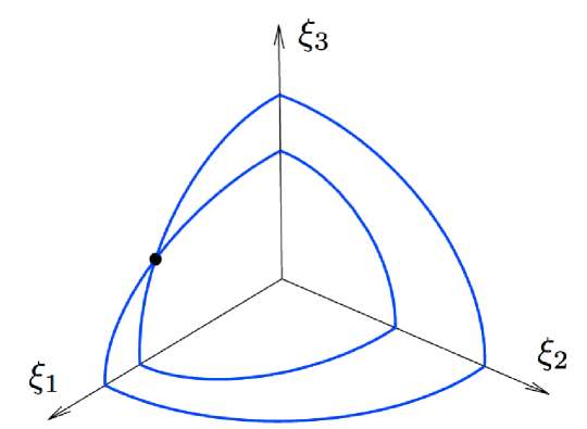
Figure 1. One quadrant in $\mathbb{R}^{3}$ of a Fresnel surface with a singular point illustrated by a dot.

Surface $S$ is defined implicitly by $f(\xi_{1},\xi_{2},\xi_{3})=0$ and singular points are characterised by $\nabla f=0$. This yields $\xi_{\operatorname{sing}}=(\sqrt{\frac{3}{2}},0,\frac{1}{\sqrt{2}})$. (For an alternative way to solve this point, see [Dah04, Lemma 4.2 (iii)].) Using computer algebra and the arguments used to prove Theorem 3.3 we may compute $\dim V_{\xi}$ when $\xi_{0}=1$ and $S$ intersects one of the coordinate planes $\{\xi_{i}=0\}_{i=1}^{3}$. In these intersections we obtain $\dim V_{\xi}=1$ except at the singular point $\xi_{\operatorname{sing}}$ where $\dim V_{\xi}=2$. $\Box$

4. Determining the medium from the Fresnel surface

As described in the introduction, the new proof of implication (iii) $\Rightarrow$ (ii) in the next theorem is the first main result of this paper. Regarding the other implications let us make a few remarks. Implication (ii) $\Rightarrow$ (i) is a standard result for the Hodge star operator on a $4$-manifold. The converse implication (i) $\Rightarrow$ (ii) is less well known. The result was first derived by Schönberg [Sch71]. For further derivations and discussions, see [Jad79, Rub02, HO03]. Below we will give yet another proof using computer algebra. The proof follows [HO03] and we use a Schönberg-Urbantke-like formula (see equations (45)–(44)) to define a metric $g$ from $\kappa$. However, the below argument that $g$ transforms as a tensor seems to be new. For a different argument, see [HO03, Section D.5.4].

When a general $2\choose 2$-tensor $\kappa$ on a $4$-manifold satisfies $\kappa^{2}=-f\operatorname{Id}$ as in condition (i) one says that $\kappa$ satisfies the closure condition. For physical motivation, see [HO03, Section D.3.1]. Let us emphasise that Theorem 4.1 is a global result. The result gives criteria for the existence of a Lorentz metric on a $4$-manifold. In general, we know that a connected manifold $M$ has a Lorentz metric if and only if $M$ is non-compact, or if $M$ is compact and the Euler number $\chi(N)$ is zero [MS08, Theorem 2.4]. Let us also note that if $J$ is an almost complex structure on a manifold $M$, that is, $J$ is a $1\choose 1$-tensor on $M$ with $J^{2}=-\operatorname{Id}$ and $\dim M\geq 2$, then $M$ is orientable [Hsi95, p. 77]. It does not seem to be known if the analogous result also holds for $2\choose 2$-tensors, that is, if the closure condition on a $4$-manifold implies orientability.

Theorem 4.1.

Suppose $N$ is an orientable $4$-manifold. If $\kappa\in\Omega^{2}_{2}(N)$ satisfies ${}^{(2)}\!\kappa=0$, then the following conditions are equivalent:

1. $\kappa^{2}=-f\operatorname{Id}$ for some function $f\in C^{\infty}(N)$ with $f>0$.

2. There exists a Lorentz metric $g$ and a nonvanishing function $f\in C^{\infty}(N)$ such that

   (40) $$\kappa = f\ast_{g}.$$

3. ${}^{(3)}\!\kappa=0$ and there exists a Lorentz metric $g$ such that

   $$F(\kappa) = F(\ast_{g}),$$

   where $F(\kappa)$ is the Fresnel surface for $\kappa$ and $F(\ast_{g})$ is the Fresnel surface for the $2\choose 2$-tensor $\ast_{g}$.

Moreover, when equivalence holds, then metrics $g$ in conditions (ii) and (iii) are conformally related.

Proof.

For implication (i) $\Rightarrow$ (ii) let $\eta=f^{-1/2}\kappa$ whence $\eta^{2}=-\operatorname{Id}$, and let $h$ be an auxiliary positive definite Riemann metric on $N$. Let $\mathscr{T}$ be an atlas given by applying Lemma 4.2 to $\eta$. For the local claim, let $(U,x^{i})$ be a chart in $\mathscr{T}$, and in this chart let $\eta$ be represented by $3\times 3$ matrices ${\mathscr{A}}$ and ${\mathscr{K}}$. With computer algebra we then obtain

(41) $${\mathscr{G}}_{h,\eta}(\xi,\xi,\xi,\xi) = \operatorname{sgn}\det{\mathscr{A}}\ (G^{ab}\xi_{a}\xi_{b})^{2},\quad\xi\in\Lambda^{1}(U),$$

where $G=(G^{ab})$ is the $4\times 4$ matrix

(44) $$G = \frac{1}{(\det h)^{1/4}}\ \frac{1}{|\det{\mathscr{A}}|^{1/2}}\left(\begin{array}[]{c|c}\det{\mathscr{A}}&k^{i}\\ \hline\cr k^{j}&-{\mathscr{A}}^{ij}+(\det{\mathscr{A}})^{-1}k^{i}k^{j},\end{array}\right),$$

and $k^{i}={\mathscr{A}}^{ib}\frac{1}{2}\varepsilon_{bcd}{\mathscr{K}}^{cd}$ for $i\in\{1,2,3\}$. Using a Shur complement [Pra94, Theorem 3.1.1] we find that

$$\det G = -\frac{1}{\det h}.$$

Hence $\det G<0$, so matrix $G$ is invertible and has constant signature $(-+++)$ or $(+---)$ in $U$. Let $G_{ij}$ be the $ij$th entry of the inverse of $G$. In $U$ we define

(45) $$g = \sigma_{U}G_{ij}dx^{i}\otimes dx^{j},$$

where constant $\sigma_{U}\in\{-1,1\}$ is chosen such that $g$ has signature $(-+++)$. Then $g$ defines a smooth symmetric $0\choose 2$-tensor in $U$ with signature $(-+++)$, and by computer algebra we have

(46) $$\eta|_{U} = -\operatorname{sgn}\operatorname{det}{\mathscr{A}}\,\ast_{g}.$$

This completes the local claim in (i) $\Rightarrow$ (ii). For the global claim, let $(U,x^{i})$ and $(\widetilde{U},\widetilde{x}^{i})$ be overlapping charts in $\mathscr{T}$, and in these charts let $G^{ij}$ and $\widetilde{G}^{ij}$ be defined as above. Since ${\mathscr{G}}_{h,\eta}$ is a tensor, equation (41) implies that

(47) $$\operatorname{sgn}\det{\mathscr{A}}\ (G^{ij}\xi_{i}\xi_{j})^{2} = \operatorname{sgn}\det\widetilde{\mathscr{A}}\ (\widetilde{G}^{ij}\frac{\partial x^{r}}{\partial\widetilde{x}^{i}}\frac{\partial x^{s}}{\partial\widetilde{x}^{j}}\xi_{r}\xi_{s})^{2}$$

for all $\xi=\xi_{i}dx^{i}\in\Lambda^{1}(U\cap\widetilde{U})$. Since $G^{ab}$ is non-degenerate we can find a $\xi$ such that the left hand side is non-zero. Thus $\operatorname{sgn}\det{\mathscr{A}}=\operatorname{sgn}\det\widetilde{\mathscr{A}}$ in $U\cap\widetilde{U}$ and $\operatorname{sgn}\det{\mathscr{A}}$ in equation (46) defines a smooth function $N\to\mathbb{R}$. By Theorem 2.3 (iii) $\Rightarrow$ (i) there exists a smooth nonvanishing function $\lambda\colon U\cap\widetilde{U}\to\mathbb{R}$ such that

$$G^{ij} = \lambda\widetilde{G}^{rs}\frac{\partial x^{i}}{\partial\widetilde{x}^{r}}\frac{\partial x^{j}}{\partial\widetilde{x}^{s}}.$$

Equation (47) implies that function $\lambda$ can only take values $\{-1,+1\}$. Thus

$$G_{ij} = \lambda\widetilde{G}_{rs}\frac{\partial\widetilde{x}^{r}}{\partial x^{i}}\frac{\partial\widetilde{x}^{s}}{\partial x^{j}}.$$

Since $\sigma_{U}G_{ij}$ and $\sigma_{\widetilde{U}}\widetilde{G}_{ij}$ both have signature $(-+++)$. It follows that $\lambda\sigma_{U}=\sigma_{\widetilde{U}}$ in $U\cap\widetilde{U}$, and equation (45) defines a tensor on $N$. This completes the proof of implication (i) $\Rightarrow$ (ii).

Implication (ii) $\Rightarrow$ (iii) follows by Propositions 2.2 and 3.6.

For the proof of implication (iii) $\Rightarrow$ (i) we first establish two subclaims:

Claim $1$. The $4\choose 0$-tensor ${\mathscr{G}}_{g,\ast g}$ is pointwise proportional to ${\mathscr{G}}_{g,\kappa}$ by a non-zero constant.

Let $p\in N$. By Proposition 3.4 we only need to show that there exists a $\lambda\in\mathbb{R}$ such that

$${\mathscr{G}}_{g,\ast g}(\xi,\xi,\xi,\xi) = \lambda{\mathscr{G}}_{g,\kappa}(\xi,\xi,\xi,\xi),\quad\xi\in\Lambda^{1}_{p}(N).$$

Let $x^{i}$ be coordinates around $p$ such that $g|_{p}=k\operatorname{diag}(1,-1,-1,-1)$ for $k\in\{\pm 1\}$. In these coordinates, let ${\mathscr{G}}^{ijkl}_{g,\ast g}$ and ${\mathscr{G}}^{ijkl}_{g,\kappa}$ be components for the symmetric $4\choose 0$-tensors ${\mathscr{G}}_{g,\ast g}|_{p}$ and ${\mathscr{G}}_{g,\kappa}|_{p}$, so that

$${\mathscr{G}}_{g,\ast g}(\xi,\xi,\xi,\xi)={\mathscr{G}}^{ijkl}_{g,\ast_{g}}\xi_{i}\xi_{j}\xi_{k}\xi_{l},\quad{\mathscr{G}}_{g,\kappa}(\xi,\xi,\xi,\xi)={\mathscr{G}}^{ijkl}_{g,\kappa}\xi_{i}\xi_{j}\xi_{k}\xi_{l}$$

for $\xi=\xi_{i}dx^{i}|_{p}$. Using these components, let $P,Q$ be the polynomials $P,Q\colon\mathbb{R}^{4}\to\mathbb{R}$,

$$P(\xi_{0},{\mbox{\boldmath$\xi$}})={\mathscr{G}}^{ijkl}_{g,\ast_{g}}\xi_{i}\xi_{j}\xi_{k}\xi_{l},\quad Q(\xi_{0},{\mbox{\boldmath$\xi$}})={\mathscr{G}}^{ijkl}_{g,\kappa}\xi_{i}\xi_{j}\xi_{k}\xi_{l},$$

where $\xi_{0}\in\mathbb{R}$, ${\mbox{\boldmath$\xi$}}=(\xi_{1},\xi_{2},\xi_{3})\in\mathbb{R}^{3}$. By Proposition 3.6,

$$P(\xi_{0},{\mbox{\boldmath$\xi$}}) = -(\xi_{0}^{2}-|{\mbox{\boldmath$\xi$}}|^{2})^{2}$$

$$= -\left(\xi_{0}-|{\mbox{\boldmath$\xi$}}|\right)^{2}\left(\xi_{0}+|{\mbox{\boldmath$\xi$}}|\right)^{2},$$

for all $(\xi_{0},{\mbox{\boldmath$\xi$}})\in\mathbb{R}^{4}$ when $|{\mbox{\boldmath$\xi$}}|$ is the Euclidean norm of $\xi$. Thus $P(1,0,0,0)\neq 0$ so $dx^{0}|_{p}\notin F_{p}(\ast_{g})=F_{p}(\kappa)$ whence ${\mathscr{G}}_{g,\kappa}^{0000}\neq 0$. For each ${\mbox{\boldmath$\xi$}}\in\mathbb{R}^{3}$, $Q(\xi_{0},{\mbox{\boldmath$\xi$}})$ is then a fourth order polynomial in $\xi_{0}$ with coefficients determined by ${\mbox{\boldmath$\xi$}}\in\mathbb{R}^{3}$. Hence there exists continuous maps

$$r_{i}\colon\mathbb{R}^{3}\to\mathbb{C},\quad i\in\{1,2,3,4\}$$

so that for all ${\mbox{\boldmath$\xi$}}\in\mathbb{R}^{3}$, $\{r_{i}({\mbox{\boldmath$\xi$}})\}_{i=1}^{4}$ are the roots of $Q(\cdot,{\mbox{\boldmath$\xi$}})$ [NP94]. For each ${\mbox{\boldmath$\xi$}}\in\mathbb{R}^{3}$ there exists a $\alpha({\mbox{\boldmath$\xi$}})\in\mathbb{R}$ such that

(48) $$Q(\xi_{0},{\mbox{\boldmath$\xi$}}) = \alpha({\mbox{\boldmath$\xi$}})\prod_{i=1}^{4}(\xi_{0}-r_{i}({\mbox{\boldmath$\xi$}})),\quad\xi_{0}\in\mathbb{R}.$$

Applying $\partial^{4}/\partial\xi_{0}^{4}$ to both sides implies that $\alpha({\mbox{\boldmath$\xi$}})={\mathscr{G}}^{0000}_{g,\kappa}$. In particular, the map ${\mbox{\boldmath$\xi$}}\mapsto\alpha({\mbox{\boldmath$\xi$}})$ is constant and non-zero. Let $\mu={\mathscr{G}}^{0000}_{g,\kappa}$. Since $P$ and $Q$ have the same zero set, there exists functions $s_{i}\colon\mathbb{R}^{3}\to\{-1,1\}$ such that

$$r_{i}({\mbox{\boldmath$\xi$}}) = s_{i}({\mbox{\boldmath$\xi$}})|{\mbox{\boldmath$\xi$}}|,\quad{\mbox{\boldmath$\xi$}}\in\mathbb{R}^{3},\,i\in\{1,2,3,4\}.$$

We know that $\mathbb{R}^{3}{\setminus\{0\}}$ is path connected. Hence $\mathbb{R}^{3}{\setminus\{0\}}$ is connected. For a contradiction, suppose that $s_{i}(\mathbb{R}^{3}{\setminus\{0\}})=\{-1,+1\}$ for some $i\in\{1,2,3,4\}$. Then $\mathbb{R}^{3}{\setminus\{0\}}=U_{+}\cup U_{-}$ for open, non-empty and disjoint sets $U_{\pm}$ defined as

$$U_{\pm} = \{{\mbox{\boldmath$\xi$}}\in\mathbb{R}^{3}{\setminus\{0\}}:\pm r_{i}({\mbox{\boldmath$\xi$}})>0\}.$$

It follows that there are constants $s_{1},s_{2},s_{3},s_{4}\in\{-1,+1\}$ such that

(49) $$r_{i}({\mbox{\boldmath$\xi$}}) = s_{i}|{\mbox{\boldmath$\xi$}}|,\quad{\mbox{\boldmath$\xi$}}\in\mathbb{R}^{3},\,i\in\{1,2,3,4\}.$$

Let $\sigma$ be the number of $s_{i}$ with $s_{i}=1$. If ${\mbox{\boldmath$\xi$}}\in\mathbb{R}^{3}{\setminus\{0\}}$, then polynomial $P(\cdot,{\mbox{\boldmath$\xi$}})$ has two distinct roots $\pm|{\mbox{\boldmath$\xi$}}|$. Hence $\sigma=0$ or $\sigma=4$ are not possible, so $\sigma\in\{1,2,3\}$ and by equation (48),

$$Q(\xi_{0},{\mbox{\boldmath$\xi$}}) = \mu\left(\xi_{0}-|{\mbox{\boldmath$\xi$}}|\right)^{\sigma}\left(\xi_{0}+|{\mbox{\boldmath$\xi$}}|\right)^{4-\sigma}$$

$$= \begin{cases}\mu\left(\xi_{0}^{4}-|{\mbox{\boldmath$\xi$}}|^{4}+2\xi_{0}|{\mbox{\boldmath$\xi$}}|(\xi_{0}^{2}-|{\mbox{\boldmath$\xi$}}|^{2})\right),&\mbox{if}\,\sigma=1,\\ \mu\,(\xi_{0}^{2}-|{\mbox{\boldmath$\xi$}}|^{2})^{2},&\mbox{if}\,\sigma=2,\\ \mu\left(\xi_{0}^{4}-|{\mbox{\boldmath$\xi$}}|^{4}-2\xi_{0}|{\mbox{\boldmath$\xi$}}|(\xi_{0}^{2}-|{\mbox{\boldmath$\xi$}}|^{2})\right),&\mbox{if}\,\sigma=3,\end{cases}$$

for all $(\xi_{0},{\mbox{\boldmath$\xi$}})\in\mathbb{R}^{4}$. Since $Q$ is a polynomial, we know that $t\mapsto Q(1,t,0,0)$ is smooth near $0$. This is only possible when $\sigma=2$, and Claim $1$ follows.

Claim $2$. At each $p\in N$ there exists a non-zero $\lambda\in\mathbb{R}$ such that $\kappa|_{p}=\lambda\ast_{g}|_{p}$.

Let $p\in N$. By Proposition 2.4 (iii) there are coordinates $x^{i}$ around $p$ such that $g|_{p}=k\operatorname{diag}(1,-1,-1,-1)$ for some $k\in\{\pm 1\}$ and ${\mathscr{A}}|_{p}$ is diagonal. For $\xi=\xi_{i}dx^{i}|_{p}$ we then have

$${\mathscr{G}}_{g,\ast_{g}}(\xi,\xi,\xi,\xi)={\mathscr{G}}^{ijkl}_{g,\ast_{g}}\xi_{i}\xi_{j}\xi_{k}\xi_{l},\quad{\mathscr{G}}_{g,\kappa}(\xi,\xi,\xi,\xi)={\mathscr{G}}^{ijkl}_{g,\kappa}\xi_{i}\xi_{j}\xi_{k}\xi_{l},$$

where ${\mathscr{G}}^{ijkl}_{g,\ast g}$ and ${\mathscr{G}}^{ijkl}_{g,\kappa}$ are components for ${\mathscr{G}}_{g,\ast_{g}}$ and ${\mathscr{G}}_{g,\kappa}$ in coordinates $x^{i}$. By Claim $1$ there exists a $\lambda\in\mathbb{R}{\setminus\{0\}}$ such that

$${\mathscr{G}}^{ijkl}_{g,\ast g} = \lambda{\mathscr{G}}^{ijkl}_{g,\kappa},\quad 0\leq i\leq j\leq k\leq l\leq 3.$$

Moreover, ${}^{(3)}\!\kappa=0$. We then have $36$ polynomial equations for $\kappa$. Using the Gröbner basis (see Appendix A) for these equations we find that the equations have a unique real solution for $\kappa$ and this solution is given by $\kappa|_{p}=\lambda^{-1/3}\ast_{g}|_{p}$. This completes the proof of Claim $2$.

By Claim $2$, there exists a map $\lambda\colon N\to\mathbb{R}{\setminus\{0\}}$ such that $\kappa=\lambda\ast_{g}$ whence $\kappa^{2}=-\lambda^{2}\operatorname{Id}$. To see that $\lambda^{2}$ is smooth it suffices to note that $\lambda^{2}=-\frac{1}{6}\operatorname{trace}\kappa^{2}$. This completes the proof of implication (iii) $\Rightarrow$ (i).

When equivalence holds, Proposition 3.6 and Theorem 2.3 imply that the Lorentz metrics in conditions (ii) and (iii) are conformally related. ∎

The next lemma was used to prove implication (i) $\Rightarrow$ (ii) in Theorem 4.1. In the proof of the lemma, Claim 1 is based on [HO03, Sections D.4–D.5].

Lemma 4.2.

Suppose $N$ is an orientable $4$-manifold and $\kappa\in\Omega^{2}_{2}(N)$. If $\kappa$ has no skewon component and $\kappa^{2}=-\operatorname{Id}$, then $N$ has an oriented atlas $\mathscr{T}$ with the following property: Each $p\in N$ can be covered with a connected chart $(U,x^{i})\in\mathscr{T}$ such that if ${\mathscr{A}},{\mathscr{B}},{\mathscr{C}},{\mathscr{D}}$ represent $\kappa$ in $U$, then

1. ${\mathscr{A}}$ is invertible in $U$.

2. In $U$ there exists a smoothly varying antisymmetric $3\times 3$ matrix ${\mathscr{K}}$ such that

   $$\quad\quad{\mathscr{B}}=-{\mathscr{A}}^{-1}\left(\operatorname{Id}+\left({\mathscr{K}}{\mathscr{A}}^{-1}\right)^{2}\right),\quad{\mathscr{C}}={\mathscr{K}}{\mathscr{A}}^{-1},\quad{\mathscr{D}}=-{\mathscr{A}}^{-1}{\mathscr{K}}.$$

Proof.

Let us first make an observations: Suppose $\{x^{i}\}_{i=0}^{3}$ are arbitrary coordinates for $N$ and ${\mathscr{A}}$, ${\mathscr{B}}$, ${\mathscr{C}},{\mathscr{D}}$ are $3\times 3$ matrices that represent $\kappa$ in these coordinates. Then Proposition 2.4 (i) implies that $\kappa^{2}=-\operatorname{Id}$ is equivalent with

(50) $${\mathscr{C}}^{2}+{\mathscr{A}}{\mathscr{B}} = -\operatorname{Id},$$

(51) $${\mathscr{B}}{\mathscr{C}}+{\mathscr{C}}^{T}{\mathscr{B}} = 0,$$

(52) $${\mathscr{C}}{\mathscr{A}}+{\mathscr{A}}{\mathscr{C}}^{T} = 0.$$

Let $\mathscr{T}_{0}$ is a maximal oriented atlas for $N$. The proof is divided into two subclaims, Claim $1$ and Claim $2$.

Claim 1. For each $p\in N$ there exists a connected chart $(U,x^{i})$ that satisfy condition (i) and there exists a chart $(W,y^{i})\in\mathscr{T}_{0}$ with $U\cap W\neq\emptyset$ such that the transition map $x^{i}\mapsto y^{i}$ is orientation preserving.

By Proposition 2.4 (ii) we can find a connected chart $(U,x^{i})$ that contains $p$ and where matrix ${\mathscr{A}}$ for $\kappa$ is diagonal at $p$. The rest of Claim $1$ is divided into four cases depending on the eigenvalues of ${\mathscr{A}}|_{p}$.

Case A. Suppose all three eigenvalues of ${\mathscr{A}}|_{p}$ are non-zero. Since eigenvalues depend continuously on the matrix entries [NP94], we can shrink $U$ and part (i) follows. Claim $1$ follows by possibly reflecting the $x^{1}$-coordinate.

Case B. Suppose ${\mathscr{A}}|_{p}$ has two non-zero eigenvalues. By permutating the coordinates (see equation (21)) we may assume that ${\mathscr{A}}|_{p}=\operatorname{diag}(a_{1},a_{2},0)$ for some $a_{1},a_{2}\neq 0$. Writing out equations (50)–(52) with computer algebra gives

$${\mathscr{C}}^{1}\,_{1}={\mathscr{C}}^{2}\,_{2}={\mathscr{C}}^{3}\,_{1}={\mathscr{C}}^{3}\,_{2}=0,\quad({\mathscr{C}}^{3}\,_{3})^{2}=-1$$

at $p$. The last equation contradicts that ${\mathscr{C}}$ is real. Case B is therefore not possible.

Case C. Suppose ${\mathscr{A}}|_{p}$ has one non-zero eigenvalue. As in Case B, we can find a chart $(U,x^{i})$ for which ${\mathscr{A}}|_{p}=\operatorname{diag}(a_{1},0,0)$ for some $a_{1}\neq 0$. Writing out equations (50)–(52) as in Case B gives

$${\mathscr{C}}^{1}\,_{1}={\mathscr{C}}^{2}\,_{1}={\mathscr{C}}^{3}\,_{1}=0,\quad{\mathscr{B}}_{11}\neq 0,\quad{\mathscr{C}}^{2}\,\,_{3}\neq 0,\quad{\mathscr{C}}^{3}\,_{2}\neq 0$$

at $p$. Let $\{\widetilde{x}^{i}\}_{i=0}^{3}$ be coordinates around $p$ defined as

$$\widetilde{x}^{0} = x^{0}+x^{3},$$

$$\widetilde{x}^{i} = x^{i},\quad i\in\{1,2,3\}.$$

In these coordinates, matrix $\widetilde{\mathscr{A}}|_{p}$ has determinant $-{\mathscr{B}}_{11}({\mathscr{C}}^{3}\,_{2})^{2}$, which is non-zero, and Claim $1$ follows as in Case $A$.

Case D. Suppose all eigenvalues of ${\mathscr{A}}|_{p}$ are zero. Then ${\mathscr{A}}|_{p}=0$ and equation (50) implies that $(\det{\mathscr{C}}|_{p})^{2}=-1$. This contradicts that ${\mathscr{C}}|_{p}$ is a real matrix. Case D is therefore not possible.

Claim 2. Let $\mathscr{T}$ be the collection of all charts $(U,x^{i})$ as in Step $1$ when $p$ ranges over all points in $N$. Then $\mathscr{T}$ satisfies the sought properties.

Let $(U,x^{i})$ and $(\widetilde{U},\widetilde{x}^{i})$ be overlapping charts in $\mathscr{T}$. By Claim 1 and [Tro94, Lemma 13.9], each chart $U$ and $\widetilde{U}$ is compatible with all charts in $\mathscr{T_{0}}_{0}$. Hence the transition map $x^{i}\mapsto\widetilde{x}^{i}$ is orientation preserving, and $\mathscr{T}$ is oriented. We know that each chart in $\mathscr{T}$ satisfies property (i), and property (ii) follows by defining ${\mathscr{K}}={\mathscr{C}}{\mathscr{A}}$. Indeed, ${\mathscr{K}}$ is antisymmetric by equation (52), and the expression for ${\mathscr{B}}$ follows by equation (50). ∎

5. Non-injectivity results

Implication (iii) $\Rightarrow$ (ii) in Theorem 4.1 shows that for a special class of medium, the Fresnel surface determines the medium up to a conformal factor. In this section we will describe results and examples where the opposite is true. In the below we will see that there are various non-uniquenesses that prevents us from determining $\kappa$ (or even the conformal class of $\kappa$) from only the Fresnel surface $F(\kappa)$.

Let us study the non-injectivity of the two maps in the diagram below:

(53) $$\kappa\quad\to\quad{\mathscr{G}}(\kappa)\quad\to\quad F(\kappa),\quad\quad\kappa\in\Omega^{2}_{2}(N),$$

where ${\mathscr{G}}(\kappa)$ is the Tamm-Rubilar $4\choose 0$-tensor density induced by $\kappa$.

5.1. Non-injectivity of leftmost map

Let us first study the non-injectivity of the leftmost map in diagram (53), that is, the map

(54) $$\kappa\quad\to\quad{\mathscr{G}}(\kappa),\quad\quad\kappa\in\Omega^{2}_{2}(N).$$

Parts (ii)–(iv) in the next theorem describe three invariances that make the map in (54) non-injective. The first two parts are well known [HO03, Section 2.2]. However, let us make three remarks regarding part (iv). First, an interpretation of part (iv) is as follows: If $F,G$ solve the sourceless Maxwell equations in medium $\kappa$, then $G,F$ solve the sourceless Maxwell equations in medium $\kappa^{-1}$. In this setting, part (iv) states that both media have the same Fresnel surfaces. Second, suppose $\ast_{g}$ is the $2\choose 2$-tensor induced by a pseudo-Riemann metric $g$. Then $\ast_{g}^{2}=\pm\operatorname{Id}$, so $\ast_{g}^{-1}=\pm\ast_{g}$, whence ${\mathscr{G}}(\ast_{g})$ and ${\mathscr{G}}(\ast_{g}^{-1})$ are always conformally related. Part (iv) states that this is not only a result for Hodge star operators, but a general result for all $2\choose 2$-tensors. Third, the proof of part (iv) is based on computer algebra. Of all the proofs in this paper, this computation is algebraicly most involved. For example, if we write out equation (55) as a text string, it requires almost $13$ megabytes of memory.

Theorem 5.1.

Suppose $\kappa\in\Omega^{2}_{2}(N)$ where $N$ is a $4$-manifold. Then

1. ${\mathscr{G}}(f\kappa)=f^{3}{\mathscr{G}}(\kappa)$ for all $f\in C^{\infty}(N)$,

2. ${\mathscr{G}}(^{(2)}\!\kappa)=0$,

3. ${\mathscr{G}}(\kappa)={\mathscr{G}}(\kappa+f\operatorname{Id})$ for all $f\in C^{\infty}(N)$,

4. ${\mathscr{G}}(\kappa^{-1})={\mathscr{G}}(-(\det\kappa)^{-1/3}\kappa)$ when $\kappa$ is invertible.

Proof.

Part (i) follows by the definition, and parts (ii)–(iii) are proven in [HO03, Section 2.2]. Therefore we only need to prove part (iv). Let $\operatorname{adj}\kappa=\det\kappa\,\kappa^{-1}$ be the adjugate of $\kappa$. By part (i) it suffices to show that

(55) $$(\det\kappa)^{2}{\mathscr{G}}^{ijkl}_{\kappa}+{\mathscr{G}}^{ijkl}_{\operatorname{adj}\kappa} = 0,\quad 0\leq i\leq j\leq k\leq l\leq 3,$$

where ${\mathscr{G}}^{ijkl}_{\kappa}$ and ${\mathscr{G}}^{ijkl}_{\operatorname{adj}\kappa}$ are components of the Tamm-Rubilar tensor densities of $\kappa$ and $\operatorname{adj}\kappa$, respectively. The motivation for rewriting the claim as in equation (55) is that now both terms are polynomials. By using the method described in Appendix B we obtain that equations (55) hold, and part (iv) follows. ∎

Theorem 5.1 (ii) shows that if we restrict the map in equation (54) to purely skewon tensors, we do not obtain an injection. The next example shows that the same map is neither an injection when restricted to tensors of purely principal type.

Example 5.2.

On $N=\mathbb{R}\times\mathbb{R}^{3}$ with coordinates $\{x^{i}\}_{i=0}^{3}$, let $\kappa$ be the $2\choose 2$-tensor defined by $3\times 3$-matrices

$${\mathscr{A}}=0_{3\times 3},\,\,\,{\mathscr{B}}=\begin{pmatrix}0&0&\lambda_{1}\\ 0&0&\lambda_{2}\\ \lambda_{1}&\lambda_{2}&\lambda_{3}\end{pmatrix},\,\,\,{\mathscr{C}}=\begin{pmatrix}-2^{-1/3}&0&\lambda_{4}\\ 0&-2^{-1/3}&\lambda_{5}\\ 0&0&2^{2/3}\end{pmatrix},\,\,\,{\mathscr{D}}={\mathscr{C}}^{T},$$

where parameters $\lambda_{1},\ldots,\lambda_{5}\in\mathbb{R}$ are arbitrary. Then $\kappa$ has only a principal part, $\det\kappa=1$, and

$${\mathscr{G}}_{h,\kappa}(\xi,\xi,\xi,\xi) = 0,\quad\xi\in\Lambda^{1}(N)$$

for any pseudo-Riemann metric $h$ on $N$. $\Box$

When proving implication (iii) $\Rightarrow$ (i) in Theorem 4.1 we need to assume that $\kappa$ has real coefficients. In fact, for $2\choose 2$-tensors with complex coefficients a decomposition into principal-, skewon-, and axion components does not seem to have been developed. The next example shows that there are non-trivial complex tensors whose Fresnel surface everywhere coincides with the Fresnel surface for the standard Minkowski metric $g_{0}=\operatorname{diag}(1,-1,-1,-1)$. (For $\kappa\in\Omega^{2}_{2}(N,\mathbb{C})$ we define the Fresnel surface using the same formulas as for real $\kappa$.)

Example 5.3.

On $N=\mathbb{R}\times\mathbb{R}^{3}$ with coordinates $\{x^{i}\}_{i=0}^{3}$, let $\kappa$ be the $2\choose 2$-tensor with complex coefficients defined by $3\times 3$-matrices

$${\mathscr{A}} = -\begin{pmatrix}\frac{1}{2z^{2}}&0&0\\ 0&2z&0\\ 0&0&z\end{pmatrix},\,\,\,\quad\quad\quad\quad\quad\quad\quad\,\,{\mathscr{B}}=-{\mathscr{A}},\quad$$

$${\mathscr{C}} = i\begin{pmatrix}\frac{1}{3z^{2}}-z&0&0\\ 0&-\frac{1}{6z^{2}}+z&0\\ 0&0&-\frac{1}{6z^{2}}\end{pmatrix},\,\,\,\quad\quad{\mathscr{D}}={\mathscr{C}},$$

where $z$ is an arbitrary function $z\colon N\to\mathbb{C}{\setminus\{0\}}$ and $i$ is the complex unit. At each $p\in N$ the Fresnel surface is then determined by

$$\xi_{0}^{2}-\xi_{1}^{2}-\xi_{2}^{2}-\xi_{3}^{2} = 0,$$

where $\xi_{i}dx^{i}\in\Lambda^{1}_{p}(N)$, and

$$\operatorname{trace}\kappa=0,\quad\det\kappa=\frac{\left(1+6z^{3}\right)^{3}\,\left(5-126z^{3}+684z^{6}-648z^{9}\right)}{46656\,\,z^{12}}.$$

From the latter equation we see that for specific values of $z$, tensor $\kappa$ can be non-invertible as a linear map $\Box$

5.2. Non-injectivity of rightmost map

The next example shows that there are skewon-free $2\choose 2$-tensors $\kappa_{1}$ and $\kappa_{2}$ that have the same Fresnel surfaces, but their Tamm-Rubilar tensors are not proportional to each other. This shows that the rightmost map in equation (53) is not injective. Let us point out that this contradicts the first proposition in [PSW09] whose proof does not analyse multiplicities of roots to the Fresnel equation.

Example 5.4.

On $N=\mathbb{R}\times\mathbb{R}^{3}$ with coordinates $\{x^{i}\}_{i=0}^{3}$, let $\kappa_{1}$ be the $2\choose 2$-tensor defined by $3\times 3$-matrices

$${\mathscr{A}}_{1}=\begin{pmatrix}0&-1&1\\ -1&-2&1\\ 1&1&-1\end{pmatrix},\,\,\,{\mathscr{B}}_{1}=\begin{pmatrix}0&\frac{1}{2}&0\\ \frac{1}{2}&0&0\\ 0&0&0\end{pmatrix},\,\,\,{\mathscr{C}}_{1}=\begin{pmatrix}0&0&0\\ 0&2&1\\ \frac{1}{2}&-\frac{1}{2}&1\end{pmatrix},\,\,\,{\mathscr{D}}_{1}={\mathscr{C}}_{1}^{T}.$$

For the Euclidean metric $g_{0}$ on $N$ we then have

$${\mathscr{G}}_{g_{0},\kappa_{1}}(\xi,\xi,\xi,\xi) = (\xi_{0}-\xi_{1})(\xi_{0}-\xi_{2})^{3},\quad\xi\in\Lambda^{1}(N).$$

To exchange the role of $\xi_{1}$ and $\xi_{2}$, we perform a coordinate change $x_{0}\mapsto x_{0}$, $x_{1}\mapsto x_{2}$, $x_{2}\mapsto x_{1}$, $x_{3}\mapsto x_{3}$. With this as motivation we define $\kappa_{2}$ as the $2\choose 2$-tensor defined by $3\times 3$-matrices

$${\mathscr{A}}_{2}=\begin{pmatrix}2&1&-1\\ 1&0&-1\\ -1&-1&1\end{pmatrix},\,\,\,{\mathscr{B}}_{2}=\begin{pmatrix}0&-\frac{1}{2}&0\\ -\frac{1}{2}&0&0\\ 0&0&0\end{pmatrix},\,\,\,{\mathscr{C}}_{2}=\begin{pmatrix}2&0&1\\ 0&0&0\\ -\frac{1}{2}&\frac{1}{2}&1\end{pmatrix},\,\,\,{\mathscr{D}}_{2}={\mathscr{C}}_{2}^{T}.$$

Then

$${\mathscr{G}}_{g_{0},\kappa_{2}}(\xi,\xi,\xi,\xi) = -(\xi_{0}-\xi_{1})^{3}(\xi_{0}-\xi_{2}),\quad\xi\in\Lambda^{1}(N).$$

Here $\kappa_{1}$ and $\kappa_{2}$ are not proportional, their Tamm-Rubilar tensor densities are not proportional, but their Fresnel surfaces coincide.

Both $\kappa_{1}$ and $\kappa_{2}$ have $1$ has an eigenvalue of algebraic multiplicity $6$. Hence

$$\det\kappa_{1}=\det\kappa_{2}=1,\quad\operatorname{trace}\kappa_{1}=\operatorname{trace}\kappa_{2}=6,$$

and for the trace-free components $\widetilde{\kappa}_{i}=\kappa_{i}-\operatorname{Id}$ we have $\det\widetilde{\kappa}_{i}=0$. $\Box$

Acknowledgements. I would like to thank Luzi Bergamin and Alberto Favaro for helpful discussions by email regarding [FB11].

The author gratefully appreciates financial support by the Academy of Finland (project 13132527 and Centre of Excellence in Inverse Problems Research), and by the Institute of Mathematics at Aalto University.

Appendix A Gröbner bases

To prove implication (iii) $\Rightarrow$ (i) in Theorem 4.1 we use a Gröbner basis to solve a system of polynomial equations. In this appendix we collect the results about Gröbner bases that are needed for this step in the proof. These results are standard and can, for example, be found in [CLO07, pp. 5, 29–32, 76–77].

By $\mathbb{C}[x]$ we denote the ring of polynomials with complex coefficient that depend on variables $x_{1},\ldots,x_{N}\in\mathbb{C}$ where $N\geq 1$. A (polynomial) ideal is a subset $I\subset\mathbb{C}[x]$ such that

1. $0\in I$,

2. $f,g\in I$ implies that $f+g\in I$,

3. $f\in I$ and $g\in\mathbb{C}[x]$ implies that $fg\in I$.

Theorem A.1 (Hilbert basis theorem).

If $I\subset\mathbb{C}[x]$ is an ideal, then there exists finitely many polynomials $f_{1},\ldots,f_{s}\in I$ such that

(56) $$I = \left\{\sum_{i=1}^{s}f_{i}g_{i}:g_{1},\ldots,g_{s}\in\mathbb{C}[x]\,\right\}.$$

When Theorem A.1 holds, we say that polynomials $f_{1},\ldots,f_{s}$ form a basis for ideal $I$. Conversely, if $f_{1},\ldots,f_{s}$ are any polynomials in $\mathbb{C}[x]$, the ideal on the right hand side in equation (56) is denoted by $\langle f_{1},\ldots,f_{s}\rangle$ and called the ideal generated by polynomials $f_{1},\ldots,f_{s}$. The affine variety defined by polynomials $f_{1},\ldots,f_{s}\in\mathbb{C}[x]$ is the subset $V(f_{1},\ldots,f_{s})\subset\mathbb{C}^{N}$,

$$V(f_{1},\ldots,f_{s}) = \{x\in\mathbb{C}^{N}:f_{1}(x)=\cdots=f_{s}(x)=0\,\,\}.$$

The next proposition gives sufficient conditions for two systems of polynomial equations to have the same solution sets.

Proposition A.2.

Suppose $f_{1},\ldots,f_{s}$ and $g_{1},\ldots,g_{t}$ are polynomials in $\mathbb{C}[x]$. If $\{f_{i}\}$ and $\{g_{i}\}$ generate the same ideal, that is,

$$\langle f_{1},\ldots,f_{s}\rangle = \langle g_{1},\ldots,g_{t}\rangle,$$

then

$$V(f_{1},\ldots,f_{s}) = V(g_{1},\ldots,g_{t}).$$

We will not give a precise definition for a Gröbner basis. The key property for Gröbner bases is collected in the next proposition.

Proposition A.3.

Let $f_{1},\ldots,f_{s}\in\mathbb{C}[x]$ be polynomials such that $\langle f_{1},\ldots,f_{s}\rangle\neq\{0\}$. Then there exists polynomials $g_{1},\ldots,g_{t}\in\mathbb{C}[x]$ such that

$$\langle f_{1},\ldots,f_{s}\rangle = \langle g_{1},\ldots,g_{t}\rangle.$$

Polynomials $g_{i}$ are called a Gröbner basis for the ideal $\langle f_{1},\ldots,f_{s}\rangle$.

Even if computation of Gröbner basis computation is supported by modern computer algebra systems, their computation can in practice be very time consuming. The motivation for using a Gröbner bases is that they typically simplify the solution process for polynomial equations. Thus one can think of Gröbner bases as a way to simplify polynomial equations without changing their solution set. This is illustrated in the next example.

Example A.4.

Let $S\subset\mathbb{R}^{3}$ be all $(x,y,z)\in\mathbb{R}^{3}$ such that

(57) $$xyz=1,\quad xz^{2}=y^{2},\quad z^{2}=xy.$$

By elementary manipulation, we see that $S=\{(1,1,1)\}$. To illustrate how to determine $S$ using a Gröbner a basis, let us first note that $S=V(f_{1},f_{2},f_{3})\cap\mathbb{R}^{3}$, where

$$f_{1}=xyz-1,\quad f_{2}=xz^{2}-y^{2},\quad f_{3}=z^{2}-xy.$$

With computer algebra we find that a Gröbner basis for $\langle f_{1},f_{2},f_{3}\rangle$ is given by

$$g_{1}=z^{3}-1,\quad g_{2}=y^{3}-z,\quad g_{3}=x-y^{2}z.$$

Propositions A.2 and A.3 imply that $V(f_{1},f_{2},f_{3})=V(g_{1},g_{2},g_{3})$. Hence $S$ coincide with real solutions to polynomial equations

(58) $$z^{3}=1,\quad y^{3}=z,\quad x=y^{2}z.$$

These last equations are easily solved and we find that $S=\{(1,1,1)\}$.

If we compare the original equations (57) to equations (58) computed by a Gröbner basis, we see that the latter ones are more easier to solve since they can be solved by backsubstitution. $\Box$

Appendix B Verifying very large polynomial identities

The proof of Theorem 5.1 (iv) reduces to proving equations (55) which consists of $35$ polynomial identities in $36$ variables. If we write out these polynomial identities as text strings, they occupy almost $13$ megabytes of memory. Due to this size, Mathematica (version 7.0.1) was not able to verify the identities in a reasonable time. In this appendix we describe a recursive method that is able to verify these identities. On a computer with two Intel E8400 $3$GHz processors and $3.7$ gigabytes of RAM the method finished in $10$ hours. The method relies on the following corollary to Taylor’s theorem with a Lagrange error term.

Proposition B.1.

Suppose $f$ is a polynomial $f\colon\mathbb{R}^{N}\to\mathbb{R}$ in variables $x_{1},\ldots,x_{N}\in\mathbb{R}$. Furthermore, suppose that

1. There exists a finite $K\in\{1,2,\ldots\}$ such that

   $$\frac{\partial^{K}f}{\partial x_{1}^{K}}(x) = 0\quad\mbox{for all}\,\,x\in\mathbb{R}^{N}.$$

2. Polynomials $Z^{0},\ldots,Z^{K-1}\colon\mathbb{R}^{N-1}\to\mathbb{R}$ defined as

   $$Z^{r}(y) = \frac{\partial^{r}f}{\partial x_{1}^{r}}(0,y),\quad\,y\in\mathbb{R}^{N-1},\quad r=0,\ldots,K-1$$

   are zero polynomials.

Then $f$ is the zero polynomial.

Proposition B.1 shows that to verify identity $f=0$ we only need to verify identities $Z^{0}=0$, $\ldots$, $Z^{K-1}=0$. Since these identities are obtained by differentiating $f$ and by setting one variable to zero, they are typically shorter and easier to manipulate than the original $f$. By recursively applying Proposition B.1, the proof of $f=0$ divides into smaller and smaller polynomial identities that eventually can be verified using Mathematica’s internal Expand routine. The implementation details are as follows. To verify $f=0$ we applied Proposition B.1 recursively until the polynomial had less than $27$ variables (out of $36$ original). For each application of Proposition B.1 we used the (non-optimal) constant $K=5$.

References

- [AMR88] R. Abraham, J.E. Marsden, and T. Ratiu, Manifolds, tensor analysis, and applications, Springer, 1988.
- [BE80] M. Born and E.Wolf, Principles of optics, Cambridge University Press, 1980.
- [BH96] D. Baldomir and P. Hammond, Geometry of electromagnetic systems, Oxford University Press, 1996.
- [CLO07] D. Cox, J. Little, and D. O’Shea, Ideals, varieties, and algorithms, Springer, 2007.
- [Dah04] M. Dahl, Contact geometry in electromagnetism, Progress in Electromagnetic Research 46 (2004), 77–104.
- [Dah06] by same author, Electromagnetic Gaussian beams using Riemannian geometry, Progress In Electromagnetics Research 60 (2006), 265–291.
- [Dah09] by same author, Electromagnetic fields from contact- and symplectic geometry, preprint (2009).
- [DKS89] T. Dray, R. Kulkarni, and J. Samuel, Duality and conformal structure, Journal of Mathematical Physics 30 (1989), no. 6, 1306–1309.
- [Ehr91] P. Ehrlich, Null cones and pseudo-Riemannian metrics, Semigroup forum 43 (1991), no. 1, 337–343.
- [FB11] A. Favaro and L. Bergamin, The non-birefringent limit of all linear, skewonless media and its unique light-cone structure, Annalen der Physik (2011).
- [HO03] F.W. Hehl and Y.N. Obukhov, Foundations of classical electrodynamics: Charge, flux, and metric, Progress in Mathematical Physics, Birkhäuser, 2003.
- [Hsi95] C. C. Hsiung, Almost complex and complex structures, World Scientific, 1995.
- [Iti05] Y. Itin, Nonbirefringence conditions for spacetime, Physical Review D 72 (2005), no. 8, 087502.
- [Jad79] A.Z. Jadczyk, Electromagnetic permeability and the vacuum and light-cone structure, Bulletin de L’Academie Polonaise des sciences — Séries des sciences physiques et astron. 27 (1979), no. 2, 91–94.
- [Kac02] A.P. Kachalov, Nonstationary electromagnetic Gaussian beams in inhomogeneous anisotropic media, Journal of Mathematical Sciences 111 (2002), no. 4, 3667–3677.
- [Kac04] by same author, Gaussian beams for Maxwell Equations on a manifold, Journal of Mathematical Sciences 122 (2004), no. 5, 3485–3501.
- [Kac05] by same author, Gaussian beams, the Hamilton-Jacobi equations, and Finsler geometry, Journal of Mathematical Sciences 127 (2005), no. 6, 2374–2388, English translation of article in Zapiski Nauchnykh Seminarov POMI, Vol. 297, 2003, pp. 66–92.
- [KKL01] A. Kachalov, Y. Kurylev, and M. Lassas, Inverse boundary spectral problems, Chapman & Hall/CRC, 2001.
- [LH04] C. Lämmerzahl and F.W. Hehl, Riemannian light cone from vanishing birefringence in premetric vacuum electrodynamics, Physical Review D 70 (2004), no. 10, 105022.
- [Low05] R.J. Low, The space of null geodesics (and a new causal boundary), Springer Lecture Notes in Physics 692 (2005), 35–50.
- [LSTV94] I.V. Lindell, A.H. Sihvola, S.A. Tretyakov, and A.J. Viitanen, Electromagnetic waves in chiral and bi-isotropic media, Artech House, 1994.
- [Mos71] H.E. Moses, Eigenfunctions of the curl operator, rotationally invariant Helmholtz theorem, and applications to electromagnetic theory and fluid mechanics, SIAM Journal of Applied Mathematics 21 (1971), no. 1, 114–144.
- [MS08] E. Minguzzi and M. Sánchez, The causal hierarchy of spacetimes, Recent Developments in Pseudo-Riemannian Geometry (D.V. Alekseevsky and H. Baum, eds.), European Mathematical Society, 2008.
- [Muj06] J. Mujica, Holomorphic functions on Banach spaces, Note di Mathematica 25 (2005/2006), no. 2, 113–138.
- [NP94] R. Naulin and C. Pabst, The roots of a polynomial depend continuously on its coefficients, Revista Colombiana de Matemáticas 28 (1994), 35–37.
- [OFR00] Y.N. Obukhov, T. Fukui, and G.F. Rubilar, Wave propagation in linear electrodynamics, Physical Review D 62 (2000), no. 4, 044050.
- [OH99] Y.N. Obukhov and F.W. Hehl, Spacetime metric from linear electrodynamics, Physics Letters B 458 (1999), 466–470.
- [OR02] Y.N. Obukhov and G.F. Rubilar, Fresnel analysis of wave propagation in nonlinear electrodynamics, Physical Review D 66 (2002), no. 2, 024042.
- [Pop02] M.M. Popov, Ray theory and Gaussian beam method for geophysicists, EDUFBA, 2002.
- [Pra94] V.V. Prasolov, Problems and theorems in linear algebra, Amererican Mathematical Society, 1994.
- [PSW09] R. Punzi, F.P. Schuller, and M.N.R. Wohlfarth, Propagation of light in area metric backgrounds, Classical and Quantum Gravity 26 (2009), 035024.
- [Ral82] J. Ralston, Gaussian beams and the propagation of singularities, Studies in partial differential equations MAA Studies in Mathematics 23 (1982), 206–248.
- [Rub02] G.F. Rubilar, Linear pre-metric electrodynamics and deduction of the light cone, Annalen der Physik 11 (2002), 717–782.
- [Sch71] M. Schönberg, Electromagnetism and gravitation, Rivista Brasileira de Fisica 1 (1971), 91–122.
- [Sco05] A. Scorpan, The wild world of 4-manifolds, AMS, 2005.
- [SWW10] F.P. Schuller, C. Witte, and M.N.R. Wohlfarth, Causal structure and algebraic classification of non-dissipative linear optical media, Annals of Physics 325 (2010), no. 9, 1853–1883.
- [Sza02] F. Szabo, Linear algebra: An introduction using Maple, Academic press, 2002.
- [Tro94] V.V. Trofimov, Introduction to geometry of manifolds with symmetry, Kluwer, 1994.