Abstract

The multiple quantum (MQ) NMR dynamics in the system of equivalent spins with the dipolar ordered initial state is considered. The high symmetry of the Hamiltonian responsible for the MQ NMR dynamics (the MQ Hamiltonian) is used in order to develop the analytical and numerical methods for an investigation of the MQ NMR dynamics in the systems consisting of hundreds of spins from ”the first principles”. We obtain the dependence of the intensities of the MQ NMR coherences on their orders (profiles of the MQ NMR coherences) for the systems of $200-600$ spins. It is shown that these profiles may be well approximated by the exponential distribution functions. We also compare the MQ NMR dynamics in the systems of equivalent spins having two different initial states, namely the dipolar ordered state and the thermal equilibrium state in the strong external magnetic field.

1 Introduction

The multiple quantum (MQ) NMR dynamics in solids [1] is extremely usefull for an investigation of solid structures and dynamical processes therein, for a counting the number of spins in impurity clusters [2, 3], for a simplification of the standard NMR spectra [4]. Usually the MQ NMR experiments deal with samples where the nuclear spin system is initially prepared in the thermal equilibrium state in the strong external magnetic field [1]. However, it is possible to carry out the MQ NMR experiments with samples prepared in different initial states [5]. In particular, one can prepare a spin system in the dipolar ordered state [6] using either the adiabatic demagnetization method in the rotating reference frame (RRF) [6, 7] or the two-pulse Broekaert-Jeener sequence [6, 8]. The MQ NMR dynamics with this initial state in small spin systems has been simulated in refs. [9, 10]. Using the dipolar ordered initial state in the MQ NMR experiment one should expect the earlier appearance of multiple spin clusters and correlations in comparison with the MQ NMR experiment with the thermal equilibrium initial state in the strong external magnetic field. In fact, the analysis of the MQ NMR experiments in the six-eight spin systems [9, 10] demonstrates that the six-eight order MQ coherences appear earlier in the experiment with the dipolar ordered initial state.

One of the basic problems for the theoretical description of the MQ NMR experiments is an exponential growth of the density matrix dimensionality with the increase in the number of spins. Therefore the modern numerical methods have been developed for simulation of the MQ NMR dynamics, which are based either on Chebyshev polynomial expansion [11] or quantum parallelism [12]. However, these methods allow one to study the MQ NMR dynamics in systems of no more than several tens of spins. A significant progress in this direction has been achieved in simulation of the MQ NMR dynamics in the system of equivalent spins [13, 14, 15], which may be prepared, for instance, filling the closed nanopore with the gas of spin-carring molecules (or atoms). The matter is that, due to the special symmetry of the Hamiltonian governing the dynamics in such spin system, it becomes possible to study the MQ NMR dynamics in systems of hundreds of spins and even more [13, 14]. The nature of the above mentioned symmetry can be clarified as follows. As far as the characteristic time between two successive collisions with the nanopore walls is several orders less that the time of mutual flip-flops of any two nuclear spins (which is defined by their dipole-dipole interaction (DDI)) [13, 14], it seems to be reasonable to use the averaged DDI, which may be obtained by averaging over the spin positions in the nanopore [13]. This means that the constant of the averaged DDI remains the same for any pair of spins in the nanopore [13], so that the nuclear spins become equivalent. For this reason, the Hamiltonian of the nuclear spin DDI in the nanopore commutes with the operator of the square of the total spin angular momentum $I^{2}$ [15, 16]. Thus, it becomes possible to use the basis of the common eigenfunctions for the operator of the square of the total spin momentum $I^{2}$ and of its projection $I_{z}$ on the direction of the external magnetic field instead of the standard multiplicative basis of the eigenfunctions of $I_{z}$, which yields an exponential growth of the Hilbert space dimensionality with the increase in the number of spins [15, 16]. As a result, we simplify calculations which allows us to succeed in both the investigation of the MQ NMR dynamics in systems of 200 – 600 spin-1/2 particles [15] and in the study of the dependence of the coherence relaxation time on the MQ NMR coherence order and the number of spins [17]. Emphasize that the nuclear spin system with the thermodynamic equilibrium initial state in the strong external magnetic field is used in refs.[15, 16, 17].

The MQ NMR dynamics in the large system of equivalent spins with the dipolar ordered initial state is studied in the present paper. The theory of MQ NMR dynamics of equivalent spins with this initial state is given in Sec.2. The dependence of the MQ NMR coherence intensities on the coherence orders (the profiles of MQ NMR coherence intensities) for systems of 200-600 spins is represented in Sec.3. The MQ NMR dynamics in systems with the dipolar ordered initial state is compared with the dynamics in systems with the thermal equilibrium initial state in the strong external magnetic field in Sec.4. The basic results are collected in Sec.5.

2 The MQ NMR coherence intensities in systems of equivalent spins prepared in the dipolar ordered initial state

We consider the system of equivalent spin-1/2 particles with the dipole-dipole interaction (DDI) in the strong external magnetic field. The secular part of the DDI Hamiltonian [6] reads:

$$H_{dz}=\sum_{j<k}D_{jk}(2I_{jz}I_{kz}-I_{jx}I_{kx}-I_{jy}I_{ky}),$$ (1)

where $D_{jk}=\frac{\gamma^{2}\hbar}{2r_{jk}^{3}}(1-3\cos^{2}\theta_{jk})$ is the constant of DDI, $\gamma$ is the gyromagnetic ratio, $r_{jk}$ is the distance between the $j$th and $k$th spins, $\theta_{jk}$ is the angle between the internuclear vector $\vec{r}_{jk}$ and the external magnetic field $\vec{B}_{0}$, and $I_{j\alpha}$ ($\alpha=x,y,z$) is the $j$th spin projection operator on the axis $\alpha$. Using either the adiabatic demagnetization in the rotating reference frame [6, 7] or the Broekaert-Jeener two-pulse sequence [6, 8] one can prepare the spin system in the dipolar ordered initial state with the following density matrix:

$$\rho(0)=\frac{1}{Z}\exp(-\beta H_{dz})\approx\frac{1}{2^{N}}(1-\beta H_{dz}),$$ (2)

where $\beta=\frac{\hbar}{kT}$ is the inverse spin temperature ($k$ is the Boltsman constant, $T$ is the temperature), $Z={\mbox{Tr}}\exp(-\beta H_{dz})$ is the partition function and $N$ is the number of spins.

If the system under consideration consists of the spin carring molecules (atoms) in the closed nanopore, then DDI is averaged (incompletely) by the fast molecular diffusion so that the constants of DDI for any spin pair equal each other, i.e. $D_{jk}\equiv D$ [13, 14]. As a result, the Hamiltonian (1) may be written as follows [14]:

$$\bar{H}_{dz}=\frac{D}{2}(3I_{z}^{2}-I^{2}),$$ (3)

where $I_{\alpha}=\sum_{i=1}^{N}I_{i\alpha}$, ($\alpha=x,y,z$), $I^{2}=I_{x}^{2}+I_{y}^{2}+I_{z}^{2}$ is the square of the spin angular momentum. It is important to justify that the high temperature approximation (2) is applicable to the system of equivalent spins. The simple analisis [18] demonstrates that approximation (2) for the system with the Hamiltonian (3) is valid if

$$\beta DN\ll 1.$$ (4)

The systems considered in our work have $N=200-600$, so that the condition (4) is satisfied.

Figure 1: The basic scheme of the four period MQ NMR experiment.

The MQ NMR experiment consists of four basic periods shown in Fig.1: the preparation period $\tau$, the evolution period $t$, the mixing period $\tau$ and the detection. The MQ NMR coherences are generated on the preparation period due to the irradiation of the sample by the multiple eight-pulse sequence of the resonance pulses [1]. Let us express MQ NMR coherences in terms of the density matrix of the preparation period. For this purpose note that the averaged Hamiltonian $\bar{H}_{MQ}$ (nonsecular two-spin/two-quantum Hamiltonian [1]) describing the MQ dynamics in the system of equivalent spins during the preparation period in the rotating reference frame may be written as follows [15, 16]:

$$\bar{H}_{MQ}=-\frac{D}{4}\{(I^{+})^{2}+(I^{-})^{2}\},$$ (5)

where $I^{+}$ and $I^{-}$ are the raising and lowering operators ($I^{\pm}=I_{x}\pm iI_{y}$). In order to investigate the MQ NMR dynamics, one has to find the density matrix $\rho(\tau)$ for the spin system solving the Liouville equation [6]:

$$i\frac{d\rho}{d\tau}=[\bar{H}_{MQ},\rho(\tau)],$$ (6)

with the initial condition $\rho(0)=\bar{H}_{dz}$. This initial condition is obtained from eqs. (2) and (3) by dropping both the unit operator and the factor ($-\beta/2^{N}$), which are not significant for the MQ NMR dynamics. Taking into account the Hamiltonians on the different periods of the MQ NMR experiment (these Hamiltonians are shown in Fig.1) one can write the expression for the dipolar energy $\langle\bar{H}_{dz}\rangle(\tau,t)$ after the mixing period of the MQ NMR experiment (Fig.1) as follows:

$$\langle\bar{H}_{dz}\rangle(\tau,t) = \frac{{\mbox{Tr}}\{U^{+}(\tau)e^{-i\Delta tI_{z}}U(\tau)\bar{H}_{dz}U^{+}(\tau)e^{i\Delta tI_{z}}U(\tau)\bar{H}_{dz}\}}{{\mbox{Tr}}\{\bar{H}_{dz}^{2}\}}=$$

$$\frac{{\mbox{Tr}}\{e^{-i\Delta tI_{z}}\rho(\tau)e^{i\Delta tI_{z}}\rho(\tau)\}}{{\mbox{Tr}}\{\bar{H}_{dz}^{2}\}},$$

where $\rho(\tau)=U(\tau)\bar{H}_{dz}U^{+}(\tau)$ is the solution to Eq.(6) and $U(\tau)=\exp(-i\bar{H}_{MQ}\tau)$. It is convenient to represent the solution to Eq.(6) as the series [19]

$$\rho(\tau)=\sum_{k}\rho_{k}(\tau),$$ (8)

where $\rho_{k}(\tau)$ obeys the relationship $[I_{z},\rho_{k}(\tau)]=k\rho_{k}(\tau)$ which can be considered as the definition of $\rho_{k}(\tau)$ (in other words, $\rho_{k}(\tau)$ collects those entries of the density matrix $\rho(\tau)$ which are responsible for the $k$th order MQ NMR coherence). Then eq.(2) reads

$$\langle\bar{H}_{dz}\rangle(\tau)=\sum_{k}e^{-ik\Delta t}\frac{{\mbox{Tr}}\{\rho_{k}(\tau)\rho_{-k}(\tau)\}}{{\mbox{Tr}}\{\bar{H}_{dz}^{2}\}}=\sum_{k}e^{-ik\Delta t}J_{k}(\tau),$$ (9)

where the $k$th order MQ NMR coherence intensity $J_{k}$ is defined as follows [19]:

$$J_{k}(\tau)=\frac{{\mbox{Tr}}\{\rho_{k}(\tau)\rho_{-k}(\tau)\}}{{\mbox{Tr}}\{\bar{H}_{dz}^{2}\}}.$$ (10)

This formula will be used in the numerical analysis of the MQ NMR coherences in Sec.3.

It is easy to write the explicit expression for ${\mbox{Tr}}\{\bar{H}_{dz}^{2}\}$. First of all, using eq. (3) we may write

$${\mbox{Tr}}\{\bar{H}_{dz}^{2}\}=\frac{D^{2}}{4}{\mbox{Tr}}(3I_{z}^{2}-I^{2})^{2}=$$ (11)

$$\frac{D^{2}}{4}{\mbox{Tr}}\{9I_{z}^{4}-3I_{z}^{2}I^{2}+I^{2}(I^{2}-3I_{z}^{2})\}=$$

$$\frac{3D^{2}}{4}{\mbox{Tr}}\{3I_{z}^{4}-I_{z}^{2}I^{2}\}=\frac{3D^{2}}{2}{\mbox{Tr}}\{I_{z}^{4}-I_{x}^{2}I_{z}^{2}\}.$$

Here we take into account that

$${\mbox{Tr}}\{I^{2}(I^{2}-3I_{z}^{2})\}=0,\;\;{\mbox{Tr}}\{I_{x}^{2}I_{z}^{2}\}={\mbox{Tr}}\{I_{y}^{2}I_{z}^{2}\}.$$ (12)

Next, it is simple to obtain the explicit expressions for ${\mbox{Tr}}\{I_{z}^{4}\}$ and ${\mbox{Tr}}\{I_{x}^{2}I_{z}^{2}\}$:

$${\mbox{Tr}}\{I_{z}^{4}\}=2^{N-4}N(3N-2),\;\;\;{\mbox{Tr}}\{I_{x}^{2}I_{z}^{2}\}=2^{N-4}N^{2}.$$ (13)

Finally, eqs.(11-13) yield the following result:

$${\mbox{Tr}}\{\bar{H}_{dz}^{2}\}=3N(N-1)2^{N-4}D^{2}.$$ (14)

Taking into account the structure of the MQ Hamiltonian $\bar{H}_{MQ}$, it may be readily shown that only the even order MQ NMR coherences appear in our numerical experiment and the coherence order may not exceed the number of spins $N$ [1, 19].

It is obvious that the MQ Hamiltonian (5) commutes with the square of the total spin momentum operator $I^{2}$ [15, 16, 17]. As far as $[I^{2},I_{z}]=0$, it is possible to use the basis of the common eigenfunctions of operators $I^{2}$ and $I_{z}$ for the description of the MQ NMR dynamics. Namely this fact allows one to avoid the problem of the exponential growth of the matrix dimensionality with the increase in the number of spins, which appears in the traditional multiplicative basis [1] of the eigenfunctions of the operator $I_{z}$. In the new basis, the MQ Hamiltonian $\bar{H}_{MQ}$ consists of blocks $\bar{H}_{MQ}^{S}$ corresponding to the different values of the total spin momentum $S$ ($\hat{S}^{2}=S(S+1)$, $S=\frac{N}{2},\frac{N}{2}-1,\frac{N}{2}-2,\cdots,\frac{N}{2}-\left[\frac{N}{2}\right]$, $[i]$ is an integer part of $i$):

$$\bar{H}_{MQ}={\mbox{diag}}\{\bar{H}^{\frac{N}{2}}_{MQ},\bar{H}^{\frac{N}{2}-1}_{MQ},\dots,\bar{H}^{\frac{N}{2}-\left[\frac{N}{2}\right]}_{MQ}\}.$$ (15)

As far as the Hamiltonian $\bar{H}_{dz}$ (3) is diagonal in the basis of the common eigenfunctions of the operators $I^{2}$ and $I_{z}$, then the density matrix $\rho(0)$ may be also splitted into the diagonal blocks $\rho^{S}(0)$ with $S=\frac{N}{2},\frac{N}{2}-1,\frac{N}{2}-2,\cdots,\frac{N}{2}-\left[\frac{N}{2}\right]$. Consequently, the matrix $\rho(\tau)$ has also the diagonal block structure with blocks $\rho^{S}(\tau)$. Thus, the problem becomes separated into the set of independent problems for each $(2S+1)\times(2S+1)$-dimensional block $\rho^{S}(\tau)$ which is a solution to the Liouville equation (6) with the Hamiltonian $\bar{H}_{MQ}^{S}$. Of course, expansion (8) may be applied to each block $\rho^{S}$. The contribution $J_{k,S}$ from the block $\rho^{S}$ to the intensity $J_{k}$ of the $k$th order coherence is defined by the obvious formula [15]:

$$J_{k,S}(\tau)=\frac{{\mbox{Tr}}\{\rho^{S}_{k}(\tau)\rho^{S}_{-k}(\tau)\}}{{\mbox{Tr}}\bar{H}_{dz}^{2}},$$ (16)

where $\rho^{S}_{k}(\tau)$ is the contribution from the matrix $\rho^{S}$ to the $k$th order coherence. One has to take into account that each block $\rho^{S}(\tau)$ is degenerated with the multiplicity $n_{N}(S)$ [20, 15]:

$$n_{N}(S)=\frac{N!(2S+1)}{(\frac{N}{2}+S+1)!(\frac{N}{2}-S)!},\;\;0\leq S\leq\frac{N}{2}.$$ (17)

As a result, the observable intensities $J_{k}(\tau)$ ($-N\leq k\leq N$) are following [15, 16]:

$$J_{k}(\tau)=\sum_{S}n_{N}(S)J_{k,S}(\tau).$$ (18)

Remember that the dimensionality of each block $\bar{H}_{MQ}^{S}$ of the MQ NMR Hamiltonian $\bar{H}_{MQ}$ is $(2S+1)$. Taking into account the block degeneration we obtain the correct value for the matrix dimensionality of both the Hamiltonina $\bar{H}_{MQ}$ and the density matrix $\rho$ [15]:

$$\sum_{S}n_{N}(S)(2S+1)=2^{N},$$ (19)

which is valid for the system of $N$ interacting spin-1/2 particles.

The numerical algorithms describing the MQ NMR dynamics in the systems of equivalent spins with the thermal equilibrium initial state in the strong external magnetic field have been developed in [15, 16, 17]. With minor corrections, these algorithms may be used for the simulation of the dynamics of the MQ NMR coherences in the spin system with the dipolar ordered initial state. In particular, the integral of motion related with the MQ NMR Hamiltonian invariance with respect to the rotation over the angle $\pi$ around $z$-axis [21] is also present. Thus, for the odd $N$, it is enough to solve the problem for the MQ NMR Hamiltonians with two times lower matrix dimensionality and then double the resulting intensities [21]. We use the spin systems with odd $N$ in all numerical calculations in the next section.

3 The numerical analysis of the MQ NMR profiles

Using the method developed in the previous section we investigate the profiles of MQ NMR coherences. As far as all spins are ”nearest neighbors” in the system of equivalent spins, $N$ spin cluster appears already after the time interval $\tau\sim 1/D$. However, some reorganization of this cluster is required for the MQ coherence formation [15]. The analysis of the MQ NMR coherence dynamics demonstrates that the quasistationary profile of MQ NMR coherences is created during $\bar{\tau}\sim 2$ ($\bar{\tau}=D\tau$ is the dimensionless time hereafter) and remains fast oscillating for $\bar{\tau}>2$. Because of these oscillations it is convenient to use the averaged intensities $\bar{J}_{k}$ [15] instead of intensities $J_{k}$ itselves. We estimate the dimensionless averaging time interval as $T\sim 2\pi/|\lambda^{min}_{3/2}|\approx 7.255$, where $\lambda^{min}_{3/2}=\sqrt{3}/2$ is the minimal eigenvalue of the Hamiltonian [15, 16]. For our convenience, we take $T=8$ so that

$$\bar{J}_{k}=\frac{1}{T}\int_{2}^{2+T}J_{k}(\bar{\tau})d\bar{\tau}.$$ (20)

It is observed that $\bar{J}_{k}$ do not significantly vary with increase in $T$, so that the definition of the averaged intensities given by eq. (20) is valid. Although the dynamics of all coherences has been found in the numerical simulations, the intensities of the high order coherences are negligible, so that we represent the intensities of the MQ NMR coherences up to the 50th order in all figures below. The profiles of MQ NMR coherence intensities for systems of 201, 401 and 601 spins with dipolar ordered initial state are shown in Fig.2. These profiles are similar to those which have been found for the systems with the thermal equilibrium initial state in the strong external magnetic field [15, 16]. Similar to refs.[15, 16], the averaged intensities of MQ NMR coherences are separated into two families:

$$\Gamma_{1}=\{\bar{J}_{4k-2},\;\;k=0,\pm 1,\pm 2,\dots\},$$ (21)

$$\Gamma_{2}=\{\bar{J}_{4k},\;\;k=\pm 1,\pm 2,\dots\},$$

with the zero order coherence intensity $\bar{J}_{0}$ does not corresponds to any of these families. Each family may be approximated by the smooth distribution function as follows:

$$\bar{J}_{2k}\approx\left\{\begin{array}[]{ll}\displaystyle A_{1}\Big{(}1+\sum_{i=1}^{4}(-1)^{i}a_{1i}(2|k|)^{i}\Big{)}e^{-2\alpha_{1}|k|},&k=\pm 1,\pm 3,\dots\cr\displaystyle A_{2}\Big{(}1+\sum_{i=1}^{6}(-1)^{i}a_{2i}(2|k|)^{i}\Big{)}e^{-2\alpha_{2}|k|},&k=\pm 2,\pm 4,\dots\cr\end{array}\right.,$$ (24)

where parameters $A_{i}$, $a_{ij}$ and $\alpha_{i}$ for spin systems with $N=201$, 401 and 601 are collected in Table 1. The algorithm defining the approximation parameters is similar to that suggested in ref.[15].

N	$A_{1}$	$a_{11}$	$a_{12}$	$a_{13}$	$a_{14}$	$\alpha_{1}$
201	$8.498\times 10^{-2}$	$3.133\times 10^{-1}$	$8.025\times 10^{-2}$	$6.109\times 10^{-3}$	$2.739\times 10^{-4}$	$2.437\times 10^{-1}$
401	$4.546\times 10^{-2}$	$1.694\times 10^{-1}$	$3.357\times 10^{-2}$	$1.649\times 10^{-3}$	$5.739\times 10^{-5}$	$1.638\times 10^{-1}$
601	$3.546\times 10^{-2}$	$1.456\times 10^{-1}$	$2.471\times 10^{-2}$	$1.028\times 10^{-3}$	$2.855\times 10^{-5}$	$1.342\times 10^{-1}$

N	$A_{2}$	$a_{21}$	$a_{22}$	$a_{23}$	$a_{24}$	$a_{25}$
201	$2.217$	$4.029\times 10^{-1}$	$7.522\times 10^{-2}$	$7.638\times 10^{-3}$	$4.624\times 10^{-4}$	$1.562\times 10^{-5}$
401	$1.411$	$3.587\times 10^{-1}$	$5.648\times 10^{-2}$	$4.616\times 10^{-3}$	$2.116\times 10^{-4}$	$5.136\times 10^{-6}$
601	$1.210$	$3.441\times 10^{-1}$	$5.123\times 10^{-2}$	$3.924\times 10^{-3}$	$1.664\times 10^{-4}$	$3.686\times 10^{-6}$

N	$a_{26}$	$\alpha_{2}$
201	$2.510\times 10^{-7}$	$3.039\times 10^{-1}$
401	$5.533\times 10^{-8}$	$2.183\times 10^{-1}$
601	$3.512\times 10^{-8}$	$1.940\times 10^{-1}$

Table 1: The parameters $A_{i}$, $a_{ij}$ and $\alpha_{i}$ of the distribution function given by eq.(24) for $N=201$, 401 and 601

Similar to the profiles of the MQ NMR coherence intensities obtained for the systems of equivalent spin-1/2 particles with the thermal equilibrium initial state in the strong external magnetic field [15], profiles for the systems with the dipolar ordered initial state seemed out to be exponential. This conclusion agrees with results obtained during an elaboration of numerous MQ NMR spectra [22] and contradicts the phenomenological theory [1] predicting the Gauss profiles of the MQ NMR coherence intensities.

Figure 2: Coherence intensities profiles for spin systems with $N=201,401,601$. The inset demonstrates that zero order coherence does not belong neither to $\Gamma_{1}$ nor to $\Gamma_{2}$. Only intensities of positive order coherences are presented.

Liouville equation (6) and formulas for the MQ NMR coherence intensities (10) yield the conservation law of the sum of the coherence intensities [23]:

$$\sum_{k}\bar{J}_{k}(\tau)=1.$$ (25)

This law together with the approximating formula (24) allows one to find a good approximation to the zero order coherence intensity. We compare the calculated values of $\bar{J}_{0}$ (see eq.(10)) with the values $\bar{J}_{0}^{appr}=1-2\sum_{k=1}^{\infty}J_{2k}$ found using the above conservation law and distribution function (24):

$$\bar{J}_{0}=\left\{\begin{array}[]{ll}2.519\times 10^{-1},&N=201\cr 2.417\times 10^{-1},&N=401\cr 2.361\times 10^{-1},&N=601\end{array}\right.,\;\;\;\bar{J}_{0}^{appr}=\left\{\begin{array}[]{ll}2.501\times 10^{-1},&N=201\cr 2.381\times 10^{-1},&N=401\cr 2.387\times 10^{-1},&N=601\end{array}\right..$$ (32)

Some discrepancy between $\bar{J}_{0}$ and $\bar{J}_{0}^{appr}$ appears because we take into account only coherences up to the 50th order in constructing the distribution function (24), while contributions from the higher order coherences are missed.

4 Comparison of the MQ NMR dynamics in the spin systems with two different initial states

The preparation of the system in the dipolar ordered initial state means that the two-spin correlations appear already at the initial time, unlike the standard MQ NMR experiment, where the thermal equilibrium initial state is defined by the one-spin Zeemann interaction with the external magnetic field [9, 10]. This statement is justified by Fig.3, where the formation times $\bar{\tau}_{f}(n)$ of different order coherences for both initial states are represented. Here the term formation time $\bar{\tau}_{f}(n)$ of the $n$th coherence means the time moment when the $n$th coherence intensity $J_{n}(\bar{\tau})$ reaches the value $\bar{J}_{n}$ for the first time. We see that MQ NMR coherences in the system with the dipolar ordered initial state (the lower solid line) appear much earlier. This result agrees with that obtained in [9] for the MQ NMR in systems with small number of spin-1/2 particles.

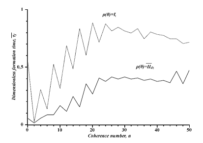
Figure 3: Coherence formation time $\bar{\tau}_{f}$ versus the coherence number for the dynamics of equivalent spins with the dipolar ordered and the thermal equilibrium in the strong external field initial states.

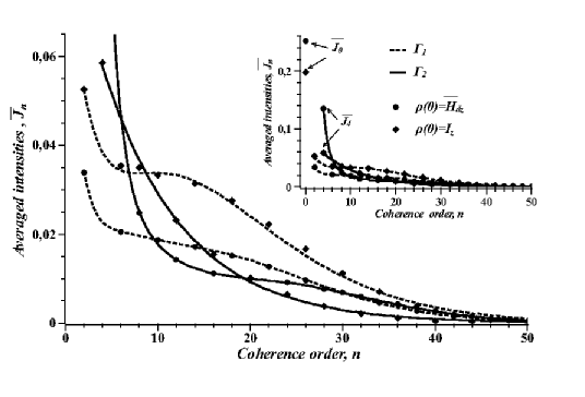
Figure 4: The MQ NMR profiles for the systems of equivalent spins with the dipolar ordered and thermal equilibrium in the strong external magnetic field initial states, $N=201$; the inset demonstrates that $\bar{J}_{0}$ and $\bar{J}_{4}$ are essentially bigger in the case of the dipolar ordered initial state.

The profiles of the MQ NMR coherence intensities for the system of $N=201$ spins with both the dipolar ordered and the thermal equilibrium in the strong magnetic field initial states are compared in Fig.4. This figure demonstrates that the discrepancy between two families of MQ NMR coherences $\Gamma_{1}$ and $\Gamma_{2}$ (see Eq.(21)) is bigger for $n<10$ and smaller for $n>10$ in the case of the dipolar ordered initial state. The inset shows that $\bar{J}_{0}$ and $\bar{J}_{4}$ are essentially bigger in the case of the dipolar ordered initial state.

Thus, similar to the usual NMR experiments in solids [6], the MQ NMR experiment in the systems of equivalent spins with the dipolar ordered initial state may be usefull to supplement the MQ NMR experiment with the thermal equilibrium initial state in the strong external magnetic field.

5 Conclusions

We have studied the MQ NMR dynamics in the systems of equivalent spin-1/2 particles with the dipolar ordered initial state. For this purpose we modify the method developed in ref.[15] for the system of equivalent spin-1/2 particles with the thermal equilibrium initial state in the strong external magnetic field. Similar to ref.[15], the high symmetry of such systems allows one to investigate the dynamics in large spin systems containing hundreds of interacting spins. We obtain dependence of the MQ NMR coherence intensities on their order (the profiles of the MQ NMR coherence intensities) in systems of 200-600 spins and demonstrate that these profiles may be well approximated by the exponential distribution functions. As far as the analogues result has been obtained in refs.[15, 16] for the systems with the thermal equilibrium initial state in the strong external magnetic field, we may suppose that the exponential profiles of MQ NMR coherence intensities are fundamental fact in MQ NMR dynamics. The theoretical results obtained in refs.[24, 25] confirm this conclusion.

We demonstrate that the MQ NMR coherences appear faster in the spin systems with the dipolar ordered initial state. The MQ NMR experiments with the dipolar ordered initial states expand possibilities of the MQ NMR spectroscopy in study of the structures of solids and the dynamical processes therein.

All numerical simulations have been performed using the resources of the Joint Supercomputer Center (JSCC) of the Russian Academy of Sciences. The work was supported by the Program of the Presidium of Russian Academy of Sciences No.21 ” Foundations of fundamental investigations of nanotechnologies and nanomaterials”.

References

- [1] J.Baum, M.Munovitz, A.N.Garroway and A.Pines, J. Chem. Phys., 83, 2015 (1985).
- [2] J.Baum, K.K.Gleason, A.Pines, A.N.Garroway and J.A.Reimer, Phys.Rev.Lett. 56, 1377 (1986).
- [3] C.E.Hughes, Prog. Nucl. Magn. Reson. Spectrosc. 45, 301 (2004)
- [4] W.S.Warren, D.P.Weitekamp and A.Pines, J. Chem. Phys. 73, 2084 (1980)
- [5] G.B.Furman and S.D.Goren, J.Phys.:Condens.Matter 17, 4501 (2005)
- [6] M. Goldman, Spin Temperature and Nuclear Magnetic Resonance in Solids (Clarendon, Oxford, 1970).
- [7] C.P.Slichter and W.C.Holton, Phys.Rev. 122, 1701 (1961)
- [8] J.Jeener and P.Broekaert, Phys. Rev. 157, 232 (1967)
- [9] S.I.Doronin, E.B.Fel’dman, E.I.Kuznetsova, G.B.Furman and S.D.Goren, Phys.Rev.B 76, 144405 (2007)
- [10] S.I.Doronin, E.B.Fel’dman, E.I.Kuznetsova, G.B.Furman and S.D.Goren, JETP Letters 86, 24 (2007)
- [11] V.V.Dobrovitski, H.A.De Raedt, M.I.Katsnelson and B.N.Harmon, Phys.Rev.Lett. 90, 210401 (2003)
- [12] W.X.Zhang, P.Cappellaro, N.Amtler, B.Pepper, D.G.Cory, V.V.Dobrovitski, C.Ramanathan and L.Viola, Phys. Rev. A 80, 052323 (2009)
- [13] J.Baugh, A.Kleinhammes, D.Han, Q.Wang and Y.Wu, Science 294, 1505 (2001)
- [14] E.B.Fel’dman and M.G.Rudavets, J.Exp.Theor.Phys. 98, 207 (2004)
- [15] S.I.Doronin, A.V.Fedorova, E.B.Fel’dman and A.I.Zenchuk, J.Chem.Phys. 131 104109 (2009)
- [16] S.I.Doronin, A.V.Fedorova, E.B.Fel’dman and A.I.Zenchuk, Phys.Chem.Chem.Phys. 12, 13273 (2010)
- [17] S.I.Doronin, E.B.Fel’dman and A.I.Zenchuk, J.Chem.Phys. 134, 034102 (2011)
- [18] F.S.Dzheparov, Preprint ITEP No. 7-10 (2010)
- [19] E.B.Fel’dman and S.Lacelle, J.Chem.Phys. 107, 7067 (1997)
- [20] L. D. Landau and E. M. Lifshitz, Course of Theoretical Physics, Vol. 3: Quantum Mechanics: Non-Relativistic Theory (Nauka, Moscow, 1974; Pergamon, New York, 1977).
- [21] S.I.Doronin, E.B.Fel’dman, I.Ya.Guinzbourg and I.I.Maximov, Chem. Phys. Lett. 341, 144 (2001).
- [22] S.Lacelle, S.-J.Hwang and B.C.Gerstein, J.Chem.Phys. 99, 8407 (1993)
- [23] D.A.Lathrop, E.S.Handy and K,K,Gleason, J.Magn.Reson. Ser.A 111, 161 (1994)
- [24] V.E.Zobov and A.A.Lundin, J.Exp.Theor.Phys. 103, 904 (2006)
- [25] V.E.Zobov and A.A.Lundin, J.Exp.Theor.Phys. 139, 519 (2011)