Gutzwiller study of extended Hubbard models with fixed boson densities

Abstract

We studied all possible ground states, including supersolid (SS) phases and phase separations of hard-core- and soft-core-extended Bose–Hubbard models with fixed boson densities by using the Gutzwiller variational wave function and the linear programming method. We found that the phase diagram of the soft-core model depends strongly on its transfer integral. Furthermore, for a large transfer integral, we showed that an SS phase can be the ground state even below or at half filling against the phase separation. We also found that the density difference between nearest-neighbor sites, which indicates the density order of the SS phase, depends strongly on the boson density and transfer integral.

I Introduction

The supersolid (SS) phase that simultaneously exhibits a superfluid (SF) phase and a density-wave order has been studied, since it was first proposed theoretically Andreev ; Chester ; Leggett . Although its existence is still controversial, a non-classical moment of inertia of solid ⁴He in Vycor glass that suggests its existence was recently reported Kim .

SS phases may also exist in optical lattices. Cold atoms in optical lattices are new experimental systems in which theoretically modeled Hamiltonians can be more distinctly simulated experimentally with no disorders. For instance, an optical lattice system, as described by a Bose–Hubbard model Fisher1 ; Jaksch , distinctly showed the phase transition between the SF phase and the Mott insulator (MI) phase Greiner . Moreover, recent observations of the long-range dipole–dipole interaction in ⁵²Cr atoms Cr may lead to the realization of the SS phase.

The simplest lattice model with a long-range interaction is the extended Bose–Hubbard model with a nearest-neighbor interaction:

$$H \ =\ H_{kin}+H_{int}^{U}+H_{int}^{V},$$

$$H_{kin} \ =\ -t\sum_{\langle i,j\rangle}(a_{i}^{\dagger}a_{j}+a_{j}^{\dagger}a_{i}),$$

$$H_{int}^{U} \ =\ \frac{U}{2}\sum_{i}n_{i}(n_{i}-1),$$

$$H_{int}^{V} \ =\ V\sum_{\langle i,j\rangle}n_{i}n_{j}.$$ (1)

Here $t$, $U$, and $V$ denote the transfer integral between nearest-neighbor sites, the repulsive intra-site interaction, and the repulsive inter-site interaction between nearest-neighbor sites, respectively. Furthermore, $a_{i}$ $(a_{i}^{\dagger})$ is the annihilation (creation) operator at the site $i$. In this study, we assume that the lattice is bipartite and consists of sublattices $A$ and $B$ and that the number of nearest-neighbor sites is $z$. The extended Bose–Hubbard model that prohibits (allows) multiple boson occupations at one site is called the hard-core (soft-core)-extended Hubbard model.

Several analytical and numerical methods exist for studying the ground state of the extended Bose–Hubbard model. The strong-coupling perturbation theory Iskin has been applied to obtain the phase boundary between the SF and non–SF phases. At least in the absence of the nearest-neighbor interaction Freericks1 ; Freericks2 , the phase boundary determined by this theory agrees perfectly with that determined by quantum Monte Carlo (QMC) simulations Scalettar1 ; Niyaz1 ; Batrouni1 ; Otterlo1 ; Capogrosso1 ; Capogrosso2 . However, this theory can neither distinguish between the SF and SS phases nor describe discontinuous transitions even if they exist. In contrast, the mean field (MF) approximation and equivalent Gutzwiller approximations Rokhsar ; Krauth can distinguish between the SF and SS phases and describe discontinuous transitions Kimura1 ; Kimura2 ; Krutitsky , although their validity is limited for high dimensions.

For the hard-core model at half filling ($N\ =\ 1/2$), both the MF approximation Matsuda ; Liu ; Scalettar2 for the mapped XXZ model and two-dimensional (2D) QMC studies Scalettar2 ; Batrouni2 identified the first-order SF–solid transition and no SS phase. The MF approximation Matsuda also showed that the transition from the SF phase to the checker-board solid phase is of the first order, and at the transition point $\mu\ =\ \mu^{*}$, the SS phase; solid phase; and PS phase in which the SS phase and the solid phase coexistx are all degenerate.

On the other hand, later QMC studies Batrouni3 ; Hebert1 showed that the SS phase is unstable against PS away from half filling.

For the soft-core model, both Gutzwiller approximations Otterlo2 ; Scarola1 and QMC simulations Scalettar2 ; Batrouni2 have shown that checker-board SS phases can be stable against the PS. However, the details of the two types of study differ. The Gutzwiller studies showed stable SS phases for both broad filling and half filling, but the PS issue is not a concern in these cases. In contrast, the 2D QMC studies did not show the SS phase at half filling but identified SS phases above half filling; however, the system energy as a function of boson density was found to be concave below half filling, which indicates a possible PS instability Scalettar2 . A later 2D QMC study Sengupta1 showed more distinctly that the SS phase is unstable against PS below half filling by exhibiting the negative compressibility $\kappa\ =\ dN/d\mu<0$. This situation is somewhat similar in one dimension (1D). Both QMC Hebert2 ; Batrouni4 and density-matrix renormalization group Kuhner1 ; Kuhner2 ; Mishra1 studies have been performed in 1D. The SS phase was found only above half filling as in the 2D case but PS did not occur Batrouni4 ; Mishra1 .

In a three-dimensional (3D) cubic lattice, Yamamoto and coworkers Yamamoto1 found some region of the parameter sets where the SS phase is stable below half filling in QMC calculations, which is consistent with a MF phase diagram on the $N$–$t/U$ plane for $V\ =\ U/6$. Hence, it is interesting to study the 3D system further. On the other hand, other previous calculations assumed a grand canonical ensemble and did not directly include the possibility that the system can be separated into two phases. As a result, the phases comprising the separate phases were not directly shown. However, if we start with a canonical ensemble and explicitly include the possibility that the system can be separated into phases, we can precisely describe the phase diagram with a fixed boson number for the entire system.

Such calculations might also be easily considered using the grand canonical ensemble if we explicitly assume that the total free energy of the system is $E_{\rm tot}\ =\ \gamma E_{\rm SS}+(1-\gamma)E_{\rm sol}$. Here $\gamma$ is the ratio of the areas of the SS phases, and we neglect the surface energy between the SS and solid phases. However, if we minimize the free energy at the chemical potential $\mu$, we can obtain only $\gamma\ =\ 0$ or 1, but not an intermediate value $0<\gamma<1$ except for $\mu\ =\ \mu^{*}$ at which the SS and solid phases are degenerate [$E_{\rm SS}(\mu^{*})\ =\ E_{\rm sol}(\mu^{*})$]. That is, the solid and SS phases cannot be in the ground state at the same time, and a separate phase including two states cannot be obtained for $\mu\ \neq\ \mu^{*}$. To obtain a separate phase, we must tune the chemical potential from $\mu$ to $\mu^{*}$; furthermore, we must try to find a $\gamma$ that satisfies the boson number condition $\gamma N_{\rm SS}+(1-\gamma)N_{\rm sol}\ =\ N$. These calculations become more complicated when the number of possible phases is large (SF, SS, MI, and several solids). This issue, in which PS can be obtained only on the phase boundary point(s) or curve(s) in the phase diagram but not for a finite region, generally occurs when we employ intensive variable(s) such as chemical potential in thermodynamics. The most popular case is the gas–liquid transition, where PS occurs only on the phase boundary curve in the pressure–volume plane for a given temperature. However, if we employ particle number, volume, and internal energy as thermodynamic variables, which are extensive quantities, we can obtain a finite region of PSs on the particle density–energy density plane.

In this study, we study the ground-state properties of the extended Bose–Hubbard model on a bipartite lattice based on the Gutzwiller approximation in a canonical ensemble; hence, we do not have to tune the chemical potential of PS. We study a wide parameter regime and present three main figures for the phase diagram on the particle density–nearest-neighbor interaction plane. Our phase diagrams for small, intermediate, and large transfer integrals differ significantly. The other main topic is the solid order parameter $\delta n\ =\ |N_{A}-N_{B}|$ [$N_{A(B)}$: the boson density on the $A(B)$ sublattice], which is also of interest and also depends strongly on the transfer integral. We employed the linear programming method numerical to minimize the total energy for a particular boson number. Following this method, we can simultaneously determine the PS region, the phases that comprise the separate phase, and the ratio of each phase to the entire system.

This paper is organized as follows, Section II introduces our calculation method, and Secs. III and IV present the hard-core and soft-core Bose–Hubbard models, respectively. Section V describes the effect of an improved calculation on the energy of the solid and MI phases. Section VI discusses the conclusions based on our results. Finally, the appendices explain the details of several perturbative calculations, the results of which are compared with the numerical results from the Gutzwiller approximation.

II CALCULATION METHOD

We employ the following Gutzwiller approximation for the SS and SF phases: $\Psi\equiv\prod_{i}\Phi_{i}$. Here, $\Phi_{i}$ is a variational wave function at the site $i$. We assume a bipartite lattice with sublattices $A$ and $B$ and a checker-board symmetry for the SS phase. The variational wave function is assumed to be $\Phi_{i}\ =\ \Phi_{A(B)}$ if the site $i$ belongs to the $A(B)$ sublattice. $\Phi_{A(B)}$ is written as a linear combination of states $|n\rangle$ with $n$ bosons as $\Phi_{A(B)}\ =\ \sum_{n}c_{A(B)n}|n\rangle$. The variational parameters $c_{A(B)n}$ are determined so as to minimize the energy expectation value. We use Powell’s method numerical to numerically optimize the variational parameters. If the result of the optimization shows $c_{An}\ \neq\ c_{Bn}$ and $c_{A(B)n}\ \neq\ \delta_{i(j)n}$, the phase is SS; however, if $c_{An}\ =\ c_{Bn}\ \neq\ \delta_{in}$, the phase is SF ($i$ and $j$ are non-negative and positive integers, respectively). The first inequality for the SS phase corresponds to the existence of a finite density difference between sublattices $A$ and $B$ $\delta n\ =\ |N_{A}-N_{B}|$ (i.e., the checker-board density order). Here $N_{A(B)}\ =\ \sum_{n}n|c_{A(B)n}|^{2}$ is the expectation value of the boson density at the $A(B)$ sublattice. The second inequality implies that the phase is not solid. For the soft-core model, in principle, the sum of $n$ must be taken from $n\ =\ 0$ to $\infty$; however, we take the sum from $n\ =\ 0$ to $n\ =\ 9$, which is sufficient for our calculation when $N\leq 1$. For the hard-core model, by definition, we consider only the two states $|n\ =\ 0\rangle$ and $|n\ =\ 1\rangle$.

The energy expectation value per site is calculated by the Gutzwiller variational wave function as

$$E \ =\ \langle H\rangle$$ (2)

$$\ =\ \langle H_{\rm kin}\rangle+\langle H_{\rm int}^{U}\rangle+\langle H_{\rm int}^{V}\rangle$$

$$\ =\ -zt\prod_{i\ =\ A,B}\sum_{n}\sqrt{n+1}c_{in}c_{i(n+1)}$$

$$+\frac{U}{4}\sum_{i\ =\ A,B}\sum_{n}n(n-1)|c_{in}|^{2}+\frac{zV}{2}N_{A}N_{B}.$$

Furthermore, we assume that the energy per site of the MI phase with $N$ bosons per site is

$$E_{\rm MI}\ =\ \frac{U}{2}N(N-1)+\frac{zV}{2}N^{2}\ =\ \frac{zV}{2}\ \ \ {\rm for}\ N\ =\ 1$$ (3)

and that of the solid phase with $N_{A}$ ($N_{B}$) bosons per site on the $A$($B$) sublattice is

$$E_{\rm S}\ =\ \frac{U}{4}\sum_{i\ =\ A,B}N_{i}(N_{i}-1)+\frac{zV}{2}N_{A}N_{B},$$ (4)

where $N_{A(B)}$ is a non-negative integer. In particular, for the solid phase when $N_{A}\ =\ 1$ and $N_{B}\ =\ 0$ (the S₁ phase), $E_{{\rm S}_{1}}\ =\ 0$; for the solid phase when $N_{A}\ =\ 2$ and $N_{B}\ =\ 0$ (the S₂ phase), $E_{{\rm S}_{2}}\ =\ U/2$. These energies correspond to those obtained from the Gutzwiller variational wave function with $c_{An}\ =\ c_{Bn}\ =\ \delta_{nN}$ for the MI phase and $c_{An}\ =\ \delta_{nN_{A}}$ and $c_{Bn}\ =\ \delta_{nN_{B}}$ ($N_{A}\ \neq\ N_{B}$) for the solid phase. Because we neglect the surface energy between different phases by assuming the thermodynamic limit, the system’s total energy per site is

$$E_{\rm tot}\ =\ \sum_{i}\gamma_{i}E_{i}$$ (5)

for the boson number condition

$$N_{\rm tot}\ =\ \sum_{i}\gamma_{i}N_{i}.$$ (6)

Here $\{E_{i}\}$ and $\{N_{i}\}$ (where $i\ =\ {\rm SF}$, SS, MI, and solids) are the energies and boson number densities, respectively, of all possible phases and $\{\gamma_{i}\}$ represent the of area or volume ratio of the phase $i$ in the entire system. Following the linear programming method numerical , we can minimize $E_{\rm tot}$ as a function of $\{\gamma_{i}\}$ note0 . Only one $\gamma_{i}$ value (corresponding to the uniform phase) or two $\gamma_{i}$ values (corresponding to PS) are automatically chosen to be nonzero as a result of minimizing $E_{\rm tot}$ because only one additional condition, the boson number condition, exists. For simplicity, however, we neglect the possibility of the separated phase that splits into the SF and SS phases, which is highly unlikely. Hereafter, we represent the separated phase consisting of phases X and Y as the PS(X + Y) phase.

III HARD-CORE MODEL

In the hard-core-extended Hubbard model, we prohibit multiple occupations at a site and define the Gutzwiller variational wave function as

$$\Phi_{A(B)}\ =\ c_{A(B)0}|0\rangle+c_{A(B)1}|1\rangle.$$ (7)

At half filling, $|c_{A(B)0}|^{2}+|c_{A(B)1}|^{2}\ =\ 1$ according to the normalization condition of the wave function, and $|c_{A1}|^{2}+|c_{B1}|^{2}\ =\ 1$ according to the boson number condition. If we set $x\ =\ c_{A0}$, then $c_{A1}\ =\ c_{B0}\ =\ \sqrt{1-x^{2}}$ and $c_{B1}\ =\ x$. Hence, the system energy per site is

$$E \ =\ -ztc_{A0}c_{A1}c_{B0}c_{B1}+\frac{zV}{2}|c_{A1}|^{2}|c_{B1}|^{2}$$ (8)

$$\ =\ \Big{(}zt-\frac{zV}{2}\Big{)}\Big{[}\Big{(}x^{2}-\frac{1}{2}\Big{)}^{2}-\frac{1}{4}\Big{]}.$$

If $V>2t$, then $x^{2}\ =\ 0$ or $1$ and the phase is S₁; however, if $V<2t$, then $x^{2}\ =\ \frac{1}{2}$ and the phase is SF. Hence, the SF–S₁ phase transition occurs at $V\ =\ 2t$ and is discontinuous. This result agrees with those of previous studies Bruder1 ; Nozieres1 .

Away from half filling, we can obtain the SF–SS phase boundary by a perturbative calculation setting $c_{A(B)n}\ =\ c_{n}+\delta c_{A(B)n}$, where $c_{n}$ is the optimized value when we assume the SF phase ($c_{An}\ =\ c_{Bn}$) and $\delta c_{A(B)n}$ represents infinitesimal quantities that describe the possible SS instability (see Appendix A.1 for details). The result is

$$V_{\rm C}\ =\ t\ \frac{N^{2}+(1-N)^{2}}{N(1-N)}.$$ (9)

That is, the energy of the SS phase is lower (higher) than that of the SF phase for $V>V_{\rm C}$ ($V<V_{\rm C}$). $V_{\rm C}^{\rm SS}$ is invariant under $N\leftrightarrow 1-N$ because of the particle–hole symmetry of the hard-core model. We also obtain the phase boundary between the SF phase and the PS(SF + S₁) phase, which consists of the SF and the S₁ phases by another perturbative calculation, assuming that the ratio of the S₁ phase to the entire system is infinitesimal (see Appendix A.2 for details). The result agrees with Eq. 9.

To determine the ground state for $V>V_{\rm C}$, we numerically compared the energy of the SS and PS(SF + S₁) phases by using the Gutzwiller variational wave function as explained in the Introduction. We found that the PS(SF + S₁) and SS phases are degenerate for $V>V_{\rm C}$ within the numerical error. The phase diagram is shown in Fig. 1. The numerical phase boundary agrees with Eq. 9 within the numerical error and the phase transitions are continuous as the perturbative calculation assumed. These results are consistent with those in Ref. Matsuda which showed that the SF–S₁ transition is of the first order and the SS, S₁, and PS(SF + S₁) phases are all degenerate at the transition point $\mu\ =\ \mu^{*}$.

We also confirmed that both $\gamma_{\rm S_{1}}$ (the ratio of the S₁ phase) in the PS(SF + S₁) phase and $\delta n\ =\ |N_{A}-N_{B}|$ in the SS phase are finite for $V>V_{\rm C}$ [Figs. 2(a) and 2(b)]. As $N$ approaches $1/2$, $\gamma_{\rm S_{1}}$ increases rapidly as a function of $(V-V_{\rm C})/V_{\rm C}$, because at half filling, no SS phase occurs and the SF–S₁ phase transition is discontinuous.

Figure 1: Phase diagram of the hard-core model. In the PS(SF + S₁)/SS phase, the SS and PS(SF + S₁) phases are degenerate. The two-dot-dashed line at half filling indicates the solid phase; the dashed line at unit filling indicates the MI phase.

Figure 2: (a) $V$ dependence of $\gamma_{\rm S_{1}}$ [the ratio of the S₁ phase in the PS(SF + S₁) phase] for $zt\ =\ 1$. (b) $\delta n\ =\ |N_{A}-N_{B}|$ in the SS phase for $zt\ =\ 1$. $V_{\rm C}$ is the critical value for the SF–PS(SF + S₁) or SF–SS transition at each value of $N$ ($zV_{\rm C}\ =\ 4.250$, 2.762, 2.167, 2.002 for $|N-1/2|\ =\ 0.3$, 0.2, 0.1, 0.01, respectively).

IV SOFT-CORE MODEL

In this section, we study the soft-core-extended Hubbard model. We employ the Gutzwiller variational wave function and optimize its variational parameters numerically. Hereafter, we call this the full numerical calculation(s); when we do not refer to the calculation method, the result was obtained by the full numerical calculations. We also perform perturbative calculations that limit the Hilbert space of the Gutzwiller variational wave function and include partial numerical calculations. We compare these perturbative calculations with the full numerical calculations. In subsection A, we examine the SS phase between the SF and solid phases at half filling. In subsection B, we examine the case away from half filling, which is the main part of this paper. Here we show that both the phase diagram on the $zV/U-N$ plane and $\delta n\ =\ |N_{A}-N_{B}|$ change qualitatively from small $zt/U$ to large $zt/U$.

IV.1 HALF FILLING

In this subsection, we primarily examine the SS phase at half filling. We compare the critical value of $V$ for the SS–S₁ transition with that of the SF–SS transition because if the former is larger than the latter, we can obtain the SS phase between the SF and S₁ phases.

By a perturbative calculation with an infinitesimal SS component added to the S₁ phase, we obtain the critical value of $V$ for the SS–S₁ transition by a power-law expansion of $zt/U$:

$$zV_{\rm C}^{\rm SS-S_{1}}\ =\ 2zt+2\frac{z^{2}t^{2}}{U}+2\frac{z^{3}t^{3}}{U^{2}}+O\Big{(}\frac{z^{4}t^{4}}{U^{3}}\Big{)}$$ (10)

(see Appendix B.1 for details). We can also obtain the critical value of $V$ for the SF–SS transition

$$zV_{\rm C}^{\rm SF-SS}\ =\ 2zt+2\frac{z^{2}t^{2}}{U}+O\Big{(}\frac{z^{4}t^{4}}{U^{3}}\Big{)},$$ (11)

by another perturbative calculation, in which an infinitesimal $\delta n\ =\ |N_{A}-N_{B}|$ is added to the SF phase (see Appendix B.2 for details). Because $V_{\rm C}^{\rm SF-SS}<V_{\rm C}^{\rm SS-S_{1}}$, the SS phase is possible for intermediate $V$ satisfying $V_{\rm C}^{\rm SF-SS}<V<V_{\rm C}^{\rm SS-S_{1}}$.

We verified these results numerically. Figure 3 shows the phase boundaries obtained by the above-mentioned perturbative calculations (dashed and dot-dashed curves) and the full numerical calculations (solid curves). A stable SS phase appears between the SF and S₁ phases. Both the SS–S₁ and SF–SS phase boundaries determined by perturbative calculations agree well with those determined by the full numerical calculations (especially at small $zt/U$ as expected). Figure 4 shows the interaction dependence of $\delta n\ =\ |N_{A}-N_{B}|$. Here, $zV_{\rm C}\ =\ zV_{\rm C}^{\rm SF-SS}$ is the critical value for the SF–SS transition at each value of $zt/U$. A finite $\delta n$ less than unity shows the density order of the SS phase, whereas $\delta n\ =\ 0(1)$ corresponds to the SF(S₁) phase. We found that $\delta n$ continuously becomes finite at the SF–SS phase transition. It changes more rapidly for smaller $zt/U$. This demonstrates that the SS phase disappears and the SF-S₁ discontinuous transition occurs in the hard core limit $zt/U\rightarrow 0$.

On the other hand, 2D QMC calculations at half filling Scalettar2 ; Batrouni2 showed that the SF phase directly transitions to the S₁ phase and no SS phase appears. However, $zt/U$ might not be sufficiently large to allow the SS phase to be easily found there, and a QMC simulation (as a matter of course, not only 2D but also 3D) for a large $zt/U$ has a possibility for finding the SS phase.

Figure 3: Phase diagram of the soft-core model at half filling. Solid curves represent numerical SF–SS and SS–S₁ phase boundaries. Dashed (dot-dashed) curve represents the SF–SS (SS–S₁) phase boundary obtained by a perturbative calculation using Eq. 11 (Eq. 10).

Figure 4: $V$ dependence of the density difference between sublattices $A$ and $B$ $\delta n\ =\ |N_{A}-N_{B}|$ in the SS phase of the soft-core model at half filling. $V_{c}$ is the critical value for the SF–SS transition at each value of $zt/U$ ($zV_{\rm C}/U\ =\ 0.219$, 0.469, 0.730 for $zt/U\ =\ 0.1$, 0.2, 0.3, respectively).

IV.2 AWAY FROM HALF FILLING

In this section, for comparison with the results of the full numerical calculations, we calculate the results of the following three perturbative equations for the phase boundary (see Appendices A, B.2, and B.3 for details). Perturbation 1 is Eq. 9, which assumes a limited Hilbert space with $|N\ =\ 0\rangle$ and $N\ =\ 1\rangle$ and is the same as that used in Sec. III; perturbation 2 is Eq. 43, which yields the SF–SS phase boundary; and perturbation 3 is Eq. 51, which yields the SF–PS(SF + S₁) or SF–PS(SF + S₂) phase boundary. For perturbations 2 and 3, we employ a limited Hilbert space with $|N\ =\ i\rangle$, where $i\ =\ 0$, 1, and 2. Hence, results obtained by perturbations 2 and 3 are expected to be better than those obtained by perturbation 1. However, perturbations 2 and 3 require a numerical calculation to minimize the SF energy in the limited Hilbert space.

We begin by analyzing the phase diagram for a small transfer integral $zt/U$. Figure 5(a) shows the phase diagram for $zt/U\ =\ 0.03$, which resembles that of the hard-core model. Namely, the upper bound of $zV/U$ for the SF phase has a minimum value near half filling, which is similar to that of the hard-core model with particle-hole symmetry. PS occurs for large $zV/U$ below half filling, and the separated phase is the PS(SF + S₁) phase, as in the hard-core model. However, the SS phase appears above half filling. These properties agree with those obtained in a 2D QMC study with $zt/U\ =\ 0.08$ Sengupta1 .

Figure 5(a) plots the result of perturbation 1 (dot-dashed curve). It agrees almost perfectly with the full numerical calculation (solid curve) except at large $N$ where the SF–SS phase boundary disappears because the PS(SS + S₂) phase appears there [see also Fig. 5(b), which expands Fig. 5(a) around $zV/U\ =\ 1$]. Both perturbation 2 for the SF–SS boundary curve and perturbation 3 for the SF–PS(SF + S₁) boundary curve yield almost the same results as perturbation 1. Therefore, they also agree almost exactly with the full numerical calculations except at large $N$.

Figure 5(b) shows that PSs also appear above half filling but the region is very small compared to that obtained by 2D QMC Sengupta1 . The appearance of the PS(SS + S₂) phase and the intricate structure of the phase diagram are non-trivial; however, the two SS phases that sandwich the PS(SS + S₂) phase have different characteristics: one having a smaller zV/U resembles the SF phase and the other having a larger zV/U resembles the S₂ phase, as we will see below through $\delta n\ =\ |N_{\rm A}-N_{\rm B}|$. Namely, SF, SS, S₂, and the PS comprising these phases are almost degenerate for $zV/U\sim 1$ above half filling.

Figure 5: Phase diagram of the soft-core model for $zt/U\ =\ 0.03$. (a) Entire phase diagram. Solid curve represents the SF–PS(SF + S₁) or SF–SS phase boundary. Dot-dashed curve for the SF–SS phase boundary obtained by the perturbative calculation in Eq. 9 cannot be distinguished from the solid curve except at large $N$, where the SF–SS transition curve disappears. (b) Expansion of (a) around $zV/U\ =\ 1$ and $N\ =\ 1$. Solid (dashed) curves for the phase boundaries show continuous (discontinuous) phase transitions. In both (a) and (b), the two-dot-dashed lines at half filling and unit filling indicate the solid phases (S₁ and S₂, respectively), and the long-dashed line at unit filling indicates the MI phase.

Figure 6 confirms that the SS phase overcomes the PS(SF + S₁) phase above half filling because the critical value of the nearest-neighbor interaction $V_{\rm C}$ for the SF–SS transition is always smaller than that for the virtual SF–PS(SF + S₁) transition. Here, the virtual SF–PS(SF + S₁) transition was obtained by setting the variational parameter of the Gutzwiller variational wave function to $c_{An}\ =\ c_{Bn}$. The difference between the curves for the SF–SS transition and the virtual SF–PS(SF + S₁) transition disappears in the hard-core limit of $zt/U\rightarrow 0$, where the SS and PS(SF + S₁) phases are degenerate, as discussed in Sec. III.

Figure 6: Critical nearest-neighbor interaction $V_{\rm C}$ for the SF–SS transition (solid curves) and the virtual SF–PS(SF + S₁) transition (dashed curves) above half filling. Note that both solid and dashed curves appear for $N\ =\ 0.6$, although they are very close.

Figure 7(a) shows the $V$ dependence of $\delta n$ obtained by the full numerical calculation. Figure 7(b) shows an expansion of the region around $1.001\leq zV/U\leq 1.002$. Note that $\delta n$ has a discontinuity at $zV_{\rm C}/U\simeq 1.001$, because the discontinuous SS–PS(SS + S₂) transition occurs there. Interestingly, the SS phase exhibits a small $\delta n$ for $zV/U\leq 1$, whereas it exhibits a large $\delta n\simeq 2N$ ($N_{A}\simeq 2N$ and $N_{B}\simeq 0$) for $zV/U\geq 1.002$ after a rapid increase in $\delta n$ in a narrow PS(SS + S₂) region ($1.001\leq zV/U\leq 1.002$), where the curves of $\delta n$ for different $N$ are almost indistinguishable [see Fig. 7(b)]. Because $\delta n\simeq 2N$, $\delta n$ is larger for larger $N$ at $zV/U\geq 1.002$. In contrast, $\delta n$ is smaller for larger $N$ for $zV/U\leq 1$, demonstrating that the critical value of $zV/U$ for the SF–SS transition is an increasing function of $N$ above half filling. The fact that $\delta n\simeq 2N$ for $zV/U\gtrsim 1$ indicates that the SS phase is similar to the S₂ phase, in which $N_{\rm A}\ =\ 2$ and $N_{\rm B}\ =\ 0$. The fact that $\delta n\simeq 0$ for $zV/U\lesssim 1$ indicates that the SS phase resembles the SF phase. Note that $zV/U\ =\ 1$ is also the phase transition point for $t\ =\ 0$ at unit filling: the MI phase (i.e., no-density-order phase) for $zV/U<1$ becomes the S₂ phase (density order phase) for $zV/U>1$. That is, even for a finite but small $t$ and $N<1$, the characteristics of the ground state change rapidly near $zV/U\simeq 1$.

Figure 7: $V$ dependence of $\delta n\ =\ |N_{A}-N_{B}|$ in the SS phase of the soft-core model for $zt/U\ =\ 0.03$. $\delta n$ is larger at smaller $N$ for $zt/U\leq 1.000$, discontinuous at $zV_{\rm C}/U\simeq 1.001$, and smaller at smaller $N$ for $zt/U\geq 1.002$. (b) Expansion around the PS(SS + S) phase ($1.001\leq zV_{\rm C}/U\leq 1.002$). In the PS(SS + S) phase, $\delta n$ is a sharply increasing function of $zV/U$, and the curves of $\delta n$ for different $N$ cannot be distinguished. Thus, the curved arrows describe the increase in $\delta n$ at each value of $N$ when we enlarge $zV/U$.

Next, we study the case of an intermediate $zt/U$ value of 0.3. Figures 8(a) and 8(b) show the phase diagram; the PS region above half filling exists, but again is very small. The phase diagram clearly departs from that of the hard-core model with the particle-hole symmetry. Interestingly, for an intermediate $zV/U$, the SS phase overcomes the PS even below half filling. This agrees with a recent 3D QMC simulation with $zt/U\ =\ 0.33$ Yamamoto1 . Figure 9 shows $\delta n$ ($\gamma_{\rm S_{1}}$) below half filling in the SS (PS(SF + S₁)) phase. The SS–PS(SF + S₁) transition is discontinuous: for $N\ =\ 0.3$, $0.35$, and $0.4$, $\delta n$ ($\gamma_{\rm S_{1}}$) is finite (zero) in the SS phase and discontinuously becomes zero (finite) in the PS(SF + S₁) phase. For $N\ =\ 0.25$, $\delta n$ is zero in the entire figure because the SS phase does not exist.

Returning to Fig. 8(a), we see that the results from perturbative calculations (dot-dashed curves) agree well with those from the full numerical calculations (solid curves). Assuming the S₁ phase for the solid, perturbation 3 is in almost perfect agreement with the SF–PS(SF + S₁) phase boundary below half filling. Perturbation 2 is also in excellent agreement with the SF–SS phase boundary except for the region of large $N\sim 1$ where the SF–SS transition becomes discontinuous, and thus cannot be described by the perturbative calculation.

Figure 8(b) shows an enlargement of Fig. 8(a) around $zV/U\ =\ 1.1$ and $N\sim 1$, where a small PS(SF + S₂) phase appears. The curve of perturbation 3 in Fig. 8(b), which is calculated assuming the S₂ phase for the solid, seems to be far from the results obtained by the full numerical calculations; however, the difference is in fact approximately 1$\%$ at most.

Figure 8: Phase diagrams of the soft-core model for $zt/U\ =\ 0.3$. (a) shows Entire phase diagram. Solid curve shows the continuous SF–PS(SF + S₁) and SF–SS transitions. Dot-dashed curves are the results of the perturbative calculations Eq. 9 (perturbation 1), Eq. 43 (perturbation 2), and Eq. 51 (perturbation 3) for the SF–PS(SF + S₁) transition. Two-dot-dashed lines at half filling and unit filling represent the solid phases (S₁ and S₂, respectively). (b) Expansion of the region around $zV/U\ =\ 1$ and $N\ =\ 1$. Solid curve shows the continuous SF–PS(SF + S₂) phase transition; dashed curve shows the discontinuous SF–SS and PS(SF + S₂)–SS phase transitions. Dot-dashed curve shows Eq. 51 (perturbation 3) for the SF–PS(SF + S₂) transition.

Figure 9: $V$ dependences of $\delta n\ =\ |N_{A}-N_{B}|$ (solid curves) and $\gamma_{\rm S_{1}}$ (dashed curves) in the soft-core model for $zt/U\ =\ 0.3$ below half-filling.

Figure 10 shows the $V$ dependence of $\delta n$ above half filling for $zt/U\ =\ 0.3$. As in Fig. 7 for $zt/U\ =\ 0.03$, $\delta n\simeq 2N$ is larger for larger $N$ at $zV/U>1.1$, whereas $\delta n$ is smaller for larger $N$ for $zV/U<1.1$. Hence, as in the case of small $zt/U$, the characteristics of the SS change drastically from SF-like to solid (S₂)-like around $zV/U\sim 1$ when we increase $zV/U$. Note that in contrast to the case of $zt/U\ =\ 0.03$, $\delta n$ shows no discontinuity except at $N\ =\ 0.9$ because the SF–SS transition is continuous. As a result, the two $\delta n$ curves for two different $N$ values intersect smoothly around $zV/U\simeq 1.1$ except at $N\ =\ 0.9$. For $N\ =\ 0.9$, $\delta n$ is zero for $zt/U<1.105$ (because the phase is SF, at which $\delta n\ =\ 0$) and discontinuously becomes finite for $zt/U>1.105$, because the SF–SS transition is discontinuous there.

Figure 10: $V$ dependence of $\delta n\ =\ |N_{A}-N_{B}|$ of the soft-core model for $zt/U\ =\ 0.3$ above half filling.

Finally, we examine a large $zt/U$($\ =\ 1$). Figure 11 shows the phase diagram. Only the SF and SS phases exist, and there are no PSs. The SF–SS transition is continuous throughout the figure. The critical $zV/U$ value between these phases is a decreasing function of the boson density $N$. This may be explained as follows. For large $zt/U$, the ratio $t$ to $V$ is the only important factor determining the phase (SF or SS, not the PS), because the lattice does not play an important role except at half or unit filling, and $N$ affects only the SF–SS phase boundary ($V$ affects the phase more strongly for larger $N$). As a result, no rapid change in the ground state properties occurs around $zV/U\ =\ 1$ in contrast to the case of small or intermediate $zt/U$.

The dot-dashed curve of perturbation 1 does not agree with the full numerical calculation (solid curve) because perturbation 1 exhibits the particle-hole symmetry of the hard-core model, which is distinctly broken here. However, the dot-dashed curve of perturbation 2 is in excellent agreement with the solid curve except at large $N$($\sim 1$).

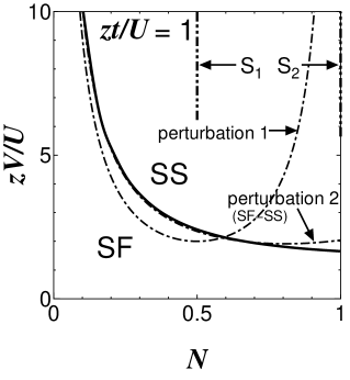
Figure 11: Phase diagram of the soft-core model for $zt/U\ =\ 1$. Solid curve represents the SF–SS phase boundary at which the phase transition is continuous. Dot-dashed curves show the results of perturbation 1 (Eq. 9) and 2 (Eq. 43). Two-dot-dashed lines at half filling and unit filling show the S₁ and S₂ phases, respectively.

Figure 12 shows the $V$ dependence of $\delta n$ in the SS phase of the soft-core model for $zt/U\ =\ 1$. $\delta n$ is larger for larger $N$ at the same $zV/U$ because the critical value of $zV/U$ for the SF–SS transition is smaller for larger $N$ (Fig. 11). Unlike the cases of $zt/U\ =\ 0.03$ (Fig. 6) or $zt/U\ =\ 0.3$ (Fig. 10), $\delta n$ is a smooth increasing function of $N$ and $zV/U$, and the two curves of $\delta n$ for two different $N$ values no longer intersect. Note that $\delta n$ does not change rapidly around $zV/U\sim 1$ as expected from the phase diagram (Fig. 11).

Figure 12: $V$ dependence of $\delta n\ =\ |N_{A}-N_{B}|$ in the soft-core model at $N\ =\ 0.3$, 0.5, 0,7, and 0.9 for $zt/U\ =\ 1$.

V Effect of improved calculation on the energy of the solid and MI phases

The energy of the solid and MI phases employed in the previous sections may be significantly higher than the exact energy. Hence, in this section, we improve the calculated energies in these phases by employing the perturbation theory Iskin up to the order of $t^{2}/U$ or $t^{2}/V$ as

$$E_{\rm MI} \ =\ \frac{zV}{2}-\frac{2zt^{2}}{U-V},$$ (12)

$$E_{\rm S_{1}} \ =\ -\frac{zt^{2}}{2(z-1)V},$$ (13)

$$E_{\rm S_{2}} \ =\ \frac{U}{2}-\frac{zt^{2}}{(2z-1)V-U}.$$ (14)

We can obtain the phase diagram by employing these improved energies. Hereafter, we assume $z\ =\ 6$ for the 3D cubic lattice. However, note that this improvement may be excessively favorable for the solid and MI phases and unfavorable for the SF and SS phases. Therefore, a correction on the order of $t^{2}/U$ or $t^{2}/V$ should also be applied to the energies of the SF and SS phases close to the SF (or SS)–solid (or MI) phase boundary. In addition, the denominators of the equations describing $E_{\rm MI}$, $E_{{\rm S}_{1}}$, and $E_{{\rm S}_{2}}$ diverge for $V\ =\ U$, $V\ =\ 0$ and $(2z-1)V\ =\ U$, respectively. Hence, we exclude the S₁ phase around $V\ =\ 0$ and the S₂ phase around $zV/U\ =\ z/(2z-1)\ =\ 6/11$. We also neglect the PS into two solids (S₁ and S₂) which is unlikely but indeed appears in this approximation. Figures 13 and 14 show the phase diagrams for $zt/U\ =\ 0.03$ and $zt/U\ =\ 0.3$, respectively. (The phase diagram for $zt/U\ =\ 1$ is the same as that in Fig. 11.) In both figures, the regions of separated phases become large, as expected. For $zt/U\ =\ 0.03$, the PS into the SF and MI phases [PS(SF + MI) phase] appears. Furthermore, for $zt/U\ =\ 0.3$, the SS phase disappears below half filling because of existence of the PS(SF + S₁) phase. These results suggest that the solid and MI energies have somewhat over-improved. On the other hand, the regions of PS into the SS and solid phases become large above half filling, which resembles the results of a 2D QMC study by Sengupta and coworkers Sengupta1 .

Figure 13: Phase diagram of the soft-core model for $zt/U\ =\ 0.03$. Energies of the solid and MI phases are improved (see text).

Figure 14: Phase diagram of the soft-core model for $zt/U\ =\ 0.3$. Energies of the solid and MI phases are improved (see text).

VI Conclusion

In this work, we studied the hard-core and soft-core-extended Hubbard models by the Gutzwiller variational wave function. We adopted a canonical ensemble and a linear programming method to include PSs more directly in our calculations. In the hard-core model away from half filling, we showed that the PS(SF + S₁) and SS phases are degenerate above a critical value of the nearest-neighbor interaction $V$, which is consistent with a previous MF study Matsuda .

Unlike the hard-core model, the soft-core model at half filling has a possible SS phase between the solid and SF phases and all the phase transitions are continuous.

Away from half filling, the phase diagram depends drastically on the transfer integral $t$. For small $zt/U$, the shape of the SF region is similar to that of the hard-core model. The PS(SF + S₁) phase appears below half filling and the SS phase appears only above half filling, as in the 2D QMC studies. For intermediate $zt/U$, the SS phase appears close to the PS below half filling as in the 3D QMC study. The phase diagram becomes simpler for large $zt/U$, where only the continuous SF–SS phase transition appears, and the critical value of $zV/U$ at the phase boundary is a smooth decreasing function of $N$.

The nearest-neighbor interaction dependence of $\delta n\ =\ |N_{A}-N_{B}|$, which shows the density wave order of the SS phase, is also interesting. For a small $zt/U$ of 0.03, $\delta n$ is a discontinuous function of $zV/U$; furthermore, the SS phase has a small $\delta n$ for small $zV/U$($\lesssim 1$) and large $\delta n$($\simeq 2N$) ($N_{A}\simeq 2N$ and $N_{B}\simeq 0$) for large $zV/U$($\gtrsim 1$). In addition, $\delta n$ is larger for smaller (larger) $N$ for $zV/U\lesssim 1$ ($zV/U\gtrsim 1$). For an intermediate $zt/U$ of 0.3, the behavior of $\delta n$ is similar to that for a small n $zt/U\ =\ 0.03$. In detail, however, unlike the case of $zt/U\ =\ 0.03$, the two curves of $\delta n$ for two different $N$ values continuously intersect around $zV/U\simeq 1.1$ because $\delta n$ is a continuous increasing function of $zV/U$ except at large $N$. For a large $zt/U\ =\ 1$, $\delta n$ is a smooth increasing function of $N$ and $zV/U$, and the two curves of $\delta n$ for two different $N$ values no longer intersect.

Throughout this paper, we found that our perturbative calculations determined the phase boundary curves very well except for large $N$($\sim 1$).

We also studied the effects of the improved perturbative calculation on the energy of the solid and MI phases. The improvement enlarges the region of PS into the SS and solid phases above half filling, which resembles the results of the 2D QMC study. However, the improvement is excessively favorable for the solid and MI phases, resulting in an unusual enlargement of the PSs. Therefore, the energies of the SF and SS phases should also be improved in future work.

Because the Gutzwiller approximation is not precise, exact numerical calculations such as QMC simulations are needed to check our results. Although some details (such as the very complicated phase diagrams for $N\sim 1$ and small $zt$) might be artifacts of our approximation, we believe that the important results in the phase diagrams and $\delta n$ values in the SS phase are worth studying in detail. For instance, the transfer integral dependence of the entire phase diagram seems to remain an open question not only in the 3D case but also in the 2D case, especially for the large $zt/U$ regime, in which an SS phase below or at half filling might exist.

Appendix A PERTURBATIVE CALCULATIONS FOR THE HARD-CORE MODEL

A.1 SF–SS TRANSITION

In the Gutzwiller approximation, the energy expectation value of the Hamiltonian (Eq. 1) is obtained as

$$E \ =\ E_{\rm kin}+E_{\rm int}^{V},$$

$$E_{\rm kin} \ =\ -ztc_{A0}c_{B0}c_{A1}c_{B1},$$

$$E_{\rm int}^{V} \ =\ \frac{zV}{2}c_{A1}^{2}c_{B1}^{2}.$$ (15)

Here, we assumed that $c_{A(B)n}$ $(n\ =\ 0,1)$ is real without the loss of generality and used $\langle a_{A(B)}\rangle\ =\ c_{A(B)0}c_{A(B)1}$ and $\langle a_{A(B)}^{\dagger}a_{A(B)}\rangle\ =\ c_{A(B)1}^{2}$. To consider a possible SS phase infinitesimally close to the SF–SS phase boundary, we set $c_{A(B)n}\ =\ c_{n}+\delta\alpha_{n}(\delta\beta_{n})$, where $\delta\alpha_{n}$ and $\delta\beta_{n}$ are infinitesimal quantities. The normalization condition of the wave function for sublattices $A$ and $B$ is written as

$$(c_{0}+\delta\alpha_{0})^{2}+(c_{1}+\delta\alpha_{1})^{2} \ =\ 1,$$

$$(c_{0}+\delta\beta_{0})^{2}+(c_{1}+\delta\beta_{1})^{2} \ =\ 1.$$ (16)

The boson number condition is written as

$$(c_{1}+\delta\alpha_{1})^{2}+(c_{1}+\delta\beta_{1})^{2}\ =\ 2N.$$ (17)

These equations can be rewritten using the normalization ($\sum_{n}c_{n}^{2}\ =\ 1$) and boson number conditions ($\sum_{n}nc_{n}^{2}\ =\ N$) in the SF phase as

$$4c_{0}\delta x_{0}+\delta x_{0}^{2}+\delta y_{0}^{2} \ =\ 0,$$

$$4c_{1}\delta x_{1}+\delta x_{1}^{2}+\delta y_{1}^{2} \ =\ 0,$$

$$c_{0}\delta y_{0}+c_{1}\delta y_{1}+\delta x_{0}\delta y_{0} \ =\ 0.$$ (18)

Here we introduced new variables $\delta x_{n}(\delta y_{n})\ =\ \delta\alpha_{n}+(-)\delta\beta_{n}$ and $\delta y_{n}\ \neq\ 0$. These equations can be further rewritten in the lowest order as

$$4c_{0}\delta x_{0}+\delta y_{0}^{2} \ =\ 0,$$

$$4c_{1}\delta x_{1}+\delta y_{1}^{2} \ =\ 0,$$

$$2c_{0}\delta y_{0}+2c_{1}\delta y_{1} \ =\ 0.$$ (19)

Hence, the value of $\delta x_{n}$ is of the same order as $\delta y_{n}^{2}$, and $\delta x_{n}$ can be rewritten in terms of $\delta y_{n}^{2}$. The energy expectation values can also be rewritten as

$$E_{\rm kin} \ =\ -zt\Big{[}N(1-N)-\frac{1}{2}(1-N)\delta y_{1}^{2}-\frac{1}{2}N\delta y_{0}^{2}\Big{]},$$

$$E_{\rm int}^{V} \ =\ \frac{zV}{2}\Big{[}N^{2}-N\delta y_{1}^{2}\Big{]}.$$ (20)

By using Eq. 18,

$$E \ =\ -zt\ N(1-N)+\frac{zt}{2}N^{2}$$ (21)

$$+\frac{1}{2}\Big{[}zt\frac{N^{2}+(1-N)^{2}}{1-N}-zVN\Big{]}\delta y_{1}^{2}.$$

If the coefficient of $\delta y_{1}^{2}$ is positive (negative), the phase is the SF (SS). By setting the coefficient of $\delta y_{1}^{2}$ equal to zero, we obtain the critical value of $V$ for the SF–SS transition

$$V_{\rm C}\ =\ t\ \frac{N^{2}+(1-N)^{2}}{N(1-N)}.$$ (22)

This is nothing but Eq. 9.

A.2 PHASE SEPARATION INTO SF AND SOLID OR MOTT PHASE

To study the PS from the SF phase into the SF phase and the S₁ (MI) phase, we set the ratio of the S₁ (MI) phase as $\gamma_{\rm SM}$. When the total boson density is $N$, the number density condition is written as

$$(1-\gamma_{\rm SM})(N-\delta N)+\gamma_{\rm SM}N_{\rm SM}\ =\ N.$$ (23)

Here $N_{\rm SM}\ =\ N_{\rm S_{1}}\ =\ 1/2$ ($N_{\rm SM}\ =\ N_{\rm MI}\ =\ 1$). If $\delta N\ =\ \gamma_{\rm SM}\ =\ 0$ the phase is the uniform SF phase. In contrast, if $\delta N,\gamma_{\rm SM}\ \neq\ 0$, the phase is the PS consisting of the SF and S₁ (MI) phases, and $N-\delta N$ is the number density of the SF phase. From Eq. 23, we obtain

$$\delta N\ \simeq\ (N_{\rm SM}-N)\gamma_{\rm SM}$$ (24)

near the SF–PS phase boundary ($\delta N\ll N$ and $\gamma_{\rm SM}\ll 1$). Because $|c_{1}|^{2}\ =\ N-\delta N$ and $|c_{0}|^{2}\ =\ 1-|c_{1}|^{2}$, the system energy per site is

$$E \ =\ \gamma_{\rm SM}E_{\rm SM}+(1-\gamma_{\rm SM})E_{\rm SF},$$

$$E_{\rm SF} \ =\ -zt|c_{0}|^{2}|c_{1}|^{2}+\frac{zV}{2}|c_{1}|^{4}$$ (25)

$$\ =\ -zt(1-N+\delta N)(N-\delta N)$$

$$+\frac{zV}{2}(N-\delta N)^{2}.$$

Here, $E_{\rm SF}$ is the energy of the SF phase and $E_{\rm SM}$ is that of the S₁ (MI) phase: $E_{\rm SM}\ =\ E_{\rm S_{1}}\ =\ 0$ ($E_{\rm SM}\ =\ E_{\rm MI}\ =\ zV/2$). To obtain the phase boundary, we substitute Eq. 24 into Eq. 25. The result is

$$E \ =\ -zt\ N(1-N)+\frac{zV}{2}N^{2}$$ (26)

$$+\Big{\{}ztN^{2}+\frac{zV}{2}N^{2}+E_{\rm SM}$$

$$+\big{[}-zVN+zt(1-2N)\big{]}N_{\rm SM}\Big{\}}\gamma_{\rm SM}$$

in the lowest order of $\gamma_{\rm SM}$. For the PS that splits into the SF and S₁ phases, $N_{\rm SM}\ =\ 1/2$, and $E_{\rm SM}\ =\ 0$. If the coefficient of $\gamma_{\rm SM}$ is positive (negative), the phase is the SF (PS). By setting the coefficient of $\gamma_{\rm SM}$ to zero, we obtain the critical value of $V$ for the PS. The result is the same as Eq. 9. In contrast, for the PS that splits into the SF and MI phases, $N_{\rm SM}\ =\ 1$, $E_{\rm SM}\ =\ zV/2$, and the coefficient of $\gamma_{\rm SM}$ is positive definite:

$$\Big{(}zt+\frac{zV}{2}\Big{)}(N-1)^{2}>0.$$ (27)

Hence, the PS into the SF and MI phases does not occur.

Appendix B PERTURBATIVE CALCULATIONS FOR THE SOFT-CORE MODEL

B.1 SS–S₁ TRANSITION AT HALF FILLING

To obtain the SS–S₁ phase boundary at half filling (Eq. 10), we set $c_{A0}\ =\ \delta\alpha_{0}$, $c_{A1}\ =\ 1-\delta\alpha_{1}$, $c_{A2}\ =\ \delta\alpha_{2}$, $c_{B0}\ =\ 1-\delta\beta_{0}$, $c_{B1}\ =\ \delta\beta_{1}$, and $c_{B2}\ =\ \delta\beta_{2}$ infinitesimally close to the phase boundary. If $\delta\alpha_{n}\ =\ \delta\beta_{n}\ =\ 0$ $(n\ =\ 0,1,2)$, the phase is SF, but if $\delta\alpha_{n},\delta\beta_{n}\ \neq\ 0$, the phase is SS. The normalization conditions of the wave function for sublattices $A$ and $B$ lead to the following equations in the lowest order:

$$\delta\alpha_{1} \ =\ \frac{1}{2}(\delta\alpha_{0}^{2}+\delta\alpha_{2}^{2}),$$

$$\delta\beta_{0} \ =\ \frac{1}{2}(\delta\beta_{1}^{2}+\delta\beta_{2}^{2}).$$ (28)

In addition, the boson number condition leads to

$$\delta\alpha_{1}\ =\ \delta\alpha_{2}^{2}+\frac{1}{2}\delta\beta_{1}^{2}+\delta\beta_{2}^{2}.$$ (29)

From these equations, we can eliminate $\delta\alpha_{0}$, $\delta\alpha_{1}$, and $\delta\beta_{0}$ and obtain the energy in terms of $\delta\alpha_{2}$, $\delta\beta_{1}$, and $\delta\beta_{2}$ as

$$E \ =\ \frac{U}{2}\delta\alpha_{2}^{2}+\frac{zV}{2}\delta\beta_{1}^{2}+\Big{(}\frac{U}{2}+zV\Big{)}\delta\beta_{2}^{2}$$ (30)

$$-zt\Big{(}\sqrt{2}\delta\alpha_{2}+\sqrt{\delta\alpha_{2}^{2}+\delta\beta_{1}^{2}+2\delta\beta_{2}^{2}}\Big{)}\delta\beta_{1}$$

$$\ =\ \Big{[}\frac{U}{2}x^{2}+\frac{zV}{2}+\Big{(}\frac{U}{2}+zV\Big{)}y^{2}$$

$$-zt\Big{(}\sqrt{2}x+\sqrt{1+x^{2}+2y^{2}}\Big{)}\Big{]}\delta\beta_{1}^{2},$$

where we have set $\delta\alpha_{2}\ =\ x\delta\beta_{1}$ and $\delta\beta_{2}\ =\ y\delta\beta_{1}$. The minimization conditions of Eq. 30 are written as

$$\frac{1}{\delta\beta_{1}^{2}}\frac{\partial E}{\partial x}\ =\ Ux-\sqrt{2}zt-\frac{ztx}{\sqrt{1+x^{2}+2y^{2}}}\ =\ 0,\ \ \ \$$ (31)

$$\frac{1}{\delta\beta_{1}^{2}}\frac{\partial E}{\partial y}\ =\ (U+2zV)y-\frac{2zty}{\sqrt{1+x^{2}+2y^{2}}}\ =\ 0.\ \ \ \$$ (32)

The latter equation leads to $y\ =\ 0$, because we assume small $zt$($\ll U$). From the former equation, we have

$$x\ =\ \frac{\sqrt{2}zt}{U}\Big{(}1+\frac{zt}{U}\Big{)}+O\Big{(}\frac{z^{3}t^{3}}{U^{3}}\Big{)}.$$ (33)

By substituting the $x$ value obtained above into Eq. 30, we obtain the optimized coefficient of $\delta\beta_{1}^{2}$. If it is positive (negative), the phase is S₁ (SS). By setting it to zero, we obtain the critical value of $zV$ for the SS–S₁ phase transition (Eq. 10).

B.2 SF–SS TRANSITION

As explained in the text, we limit the Hilbert space to three states $|0\rangle$, $|1\rangle$, and $|2\rangle$. Furthermore, we set $c_{An}\ =\ c_{n}+\delta\alpha_{n}$ and $c_{Bn}\ =\ c_{n}+\delta\beta_{n}$ where $\delta\alpha_{n}$ and $\delta\beta_{n}$ ($n\ =\ 0$, 1, 2) are infinitesimal quantities. We determine the $c_{n}$ ($n\ =\ 0$, 1, 2) value required to minimize the energy of the SF phase ($\delta\alpha_{n}\ =\ \delta\beta_{n}\ =\ 0$). As in the hard-core model (Appendix A.1), we introduce $\delta x_{n}(\delta y_{n})\ =\ \delta\alpha_{n}+(-)\delta\beta_{n}$, where $\delta y_{n}\ \neq\ 0$ for the SS phase. The wave function normalization and boson number conditions lead to

$$c_{0}\delta x_{0}+c_{1}\delta x_{1}+c_{2}\delta x_{2}\ =\ -\frac{1}{4}(\delta y_{0}^{2}+\delta y_{1}^{2}+\delta y_{2}^{2}),\ \ \ \$$

$$2c_{1}\delta x_{1}+4c_{2}\delta x_{2}\ =\ -\frac{\delta y_{1}^{2}}{2}-\delta y_{2}^{2},\ \ \ \$$

$$c_{0}\delta y_{0}+c_{1}\delta y_{1}+c_{2}\delta y_{2}\ =\ 0\ \ \ \$$ (34)

in the lowest order of $\delta x_{n}$ and $\delta y_{n}$ ($\delta x_{n}$ are of the order of $\delta y_{n}^{2}$). By eliminating $\delta x_{0}$, $\delta x_{1}$, and $\delta y_{1}^{2}$ in the above equations, we can write the energy per site in terms of $\delta x_{2}$, $\delta y_{0}$, and $\delta y_{2}$ as

$$E \ =\ E_{\rm kin}+E_{\rm int}^{U}+E_{\rm int}^{V},$$

$$E_{\rm kin} \ =\ -zt\Big{[}c_{1}^{2}\big{(}\sqrt{2}c_{2}+c_{0}\big{)}^{2}+X\delta x_{2}$$

$$-\frac{1}{4}\big{(}a_{0}\delta y_{0}^{2}+a_{02}\delta y_{0}\delta y_{2}+a_{2}\delta y_{2}^{2}\big{)}\Big{]},$$

$$E_{\rm int}^{U} \ =\ U\Big{[}c_{2}^{2}+c_{2}\delta x_{2}+\frac{1}{4}\delta y_{2}^{2}\Big{]},$$

$$E_{\rm int}^{V} \ =\ \frac{zV}{2}\Big{[}\big{(}c_{1}^{2}+2c_{2}^{2}\big{)}^{2}-\big{(}c_{0}\delta y_{0}-c_{2}\delta y_{2}\big{)}^{2}\Big{]},\ \ \$$ (35)

where

$$X \ =\ \big{(}\sqrt{2}c_{2}+c_{0}\big{)}\Big{[}c_{1}^{2}\Big{(}\sqrt{2}+\frac{c_{2}}{c_{0}}\Big{)}$$ (36)

$$-2c_{2}\big{(}\sqrt{2}c_{2}+c_{0}\big{)}\Big{]},$$

$$a_{0} \ =\ \Big{(}2+\frac{\sqrt{2}c_{2}}{c_{0}}\Big{)}c_{1}^{2}+\frac{2c_{0}^{2}}{c_{1}^{2}}\big{(}\sqrt{2}c_{2}+c_{0}\big{)}^{2},$$ (37)

$$a_{02} \ =\ 2\Big{[}\sqrt{2}c_{1}^{2}+\frac{2c_{0}c_{2}}{c_{1}^{2}}\big{(}\sqrt{2}c_{2}+c_{0}\big{)}^{2}\Big{]},$$ (38)

$$a_{2} \ =\ 2\big{(}\sqrt{2}c_{2}+c_{0}\big{)}^{2}\Big{(}1+\frac{c_{2}^{2}}{c_{1}^{2}}\Big{)}$$ (39)

$$+c_{1}^{2}\Big{(}1-\frac{\sqrt{2}c_{2}}{c_{0}}\Big{)}.$$

The total coefficient of $\delta x_{2}$ for $E$ in Eq. 35 is zero, because the variation in $\delta x_{n}$ corresponds to that in $c_{n}$ in the SF phase and the values of $c_{n}$ were already determined to minimize $E$. To be concrete, the energy of the SF phase is represented by $c_{2}$ when $\delta y_{n}\ =\ 0$ as

$$E_{\rm SF} \ =\ -zt(N-2c_{2}^{2})\Big{(}\sqrt{2}c_{2}+\sqrt{1-N+c_{2}^{2}}\Big{)}^{2}$$ (40)

$$+\frac{zV}{2}N^{2}+Uc_{2}^{2},$$

where $c_{0}$ and $c_{1}$ were already eliminated by the the wave function normalization and boson number conditions. The minimization condition $dE_{\rm SF}/dc_{2}\ =\ 0$ leads to

$$Uc_{2} \ =\ zt\Big{[}c_{2}\left(\sqrt{2}c_{2}+\sqrt{1-N+c_{2}^{2}}\right)^{2}$$ (41)

$$+\frac{N-2c_{2}^{2}}{\sqrt{1-N+c_{2}^{2}}}\left(\sqrt{2}c_{2}+\sqrt{1-N+c_{2}^{2}}\right)$$

$$\times\left(c_{2}+\sqrt{2(1-N+c_{2}^{2})}\right)\Big{]},$$

and we can easily verify that the total coefficient of $\delta x_{2}$ for $E$ in Eq. 35 is zero. $E$ is further rewritten as

$$E \ =\ {\rm const.}+A\delta y_{0}^{2}+B\delta y_{0}\delta y_{2}+C\delta y_{2}^{2},$$

$$A \ =\ \frac{zt}{4}a_{0}-\frac{zV}{2}c_{0}^{2},$$

$$B \ =\ \frac{zt}{4}a_{02}+zVc_{0}c_{2},$$

$$C \ =\ \frac{zt}{4}a_{2}-\frac{zV}{2}c_{2}^{2}+\frac{U}{4}.$$ (42)

Hence, $\delta y_{n}$ becomes finite and the phase becomes SS when $B^{2}>4AC$, which corresponds to $V>V_{\rm C}^{\rm SF-SS}$, where

$$V_{\rm C}^{\rm SF-SS} \ =\ \frac{t}{8}\frac{zt(4a_{0}a_{2}-a_{02}^{2})+4Ua_{0}}{zt(c_{2}^{2}a_{0}+c_{0}c_{2}a_{02}+c_{0}^{2}a_{2})+Uc_{0}^{2}}.\ \$$ (43)

To obtain the numerical value of Eq. 43, we numerically calculate the value of $c_{2}$ that minimizes $E$ (Eq. 40) and determine $c_{0}$ by using the normalization and boson number conditions. By replacing $c_{0}$ and $c_{2}$ in Eq. 43, we obtain the critical value $V_{\rm C}^{\rm SF-SS}$.

On the other hand, at half filling, we analytically obtain a power-law expansion of $zt/U$ for $V_{\rm C}^{\rm SF-SS}$ (Eq. 11). We start from the minimization condition obtained from Eq. 40 up to the second order of $c_{2}$:

$$\frac{dE}{dc_{2}}\ =\ -zt(1+c_{2}-9c_{2}^{2})+2Uc_{2}\ =\ 0.$$ (44)

From the above equation, we obtain $c_{2}\ =\ zt/(2U)+z^{2}t^{2}/(4U^{2})$. We determine $c_{0}$ and $c_{1}$ by $c_{2}$ through the normalization and boson number conditions. Now, $a_{0}$, $a_{02}$, and $a_{2}$ are written as

$$a_{0} \ =\ 2+5\delta+13\delta^{2},$$

$$a_{02} \ =\ \sqrt{2}(1+2\delta+6\delta^{2}),$$

$$a_{2} \ =\ \frac{3}{2}(1+2\delta+6\delta^{2}),$$ (45)

respectively, where $\delta\ =\ zt/(2U)$. By substituting $a_{0}$, $a_{02}$, and $a_{2}$ into Eq. 43, we obtain Eq. 11.

B.3 PHASE SEPARATION INTO THE SF AND SOLID OR MOTT PHASE

As explained in the text and in Appendix B. 2, we limit the Hilbert space to three states: $|0\rangle$, $|1\rangle$, and $|2\rangle$. We assume that $c_{n}\ =\ c_{n}^{(0)}$ (where $n\ =\ 0$, 1, 2) is determined to minimize the total energy of the SF phase (not the separated phase). The wave function normalization and boson number conditions are written as $\sum_{n}c_{n}^{(0)2}\ =\ 1$ and $\sum_{n}nc_{n}^{(0)2}\ =\ N$, respectively. For the separated phase, we set $c_{i}\rightarrow c_{n}^{(0)}+\delta c_{n}$ and $N\rightarrow N-\delta N$ for the SF phase in the separated phase and $\gamma_{\rm SM}$ as the ratio of the solid (or MI) phase to the entire system. As in a similar calculation in Appendix A.2, the boson number condition in the entire system is written as $\delta N\ =\ \gamma_{\rm SM}(N_{\rm SM}-N)$ in the lowest order of $\gamma_{\rm SM}$, where $N_{\rm SM}\ =\ 1/2$ (1) for the solid S₁ (S₂) phase and $N_{\rm SM}\ =\ 1$ for the MI phase. The normalization and boson number conditions for the SF phase in the separated phase are written as $\sum_{n}(c_{n}^{(0)}+\delta c_{n})^{2}\ =\ 1$ and $\sum_{n}n(c_{n}^{(0)}+\delta c_{n})^{2}\ =\ N-\delta N$, respectively. These equations are rewritten as

$$\delta c_{0} \ =\ -\frac{1}{4c_{0}}\big{(}2c_{1}\delta c_{1}-\delta N\big{)},$$

$$\delta c_{2} \ =\ -\frac{1}{4c_{2}}\big{(}2c_{1}\delta c_{1}+\delta N\big{)}.$$ (46)

From these equations and the minimization condition for $E_{\rm SF}$ (Eq. 41), we determine the energy of the SF phase $E_{\rm SF}$ in the separated phase as

$$E_{\rm SF} \ =\ -zt(N-2c_{2}^{2})\Big{(}\sqrt{2}c_{2}+\sqrt{1-N+c_{2}^{2}}\Big{)}^{2}$$ (47)

$$+\frac{zV}{2}N^{2}+Uc_{2}^{2}+Y\delta N,$$

where

$$Y \ =\ -\frac{zt}{2}c_{1}^{2}(\sqrt{2}c_{2}+c_{0})\Big{(}-\frac{\sqrt{2}}{c_{2}}+\frac{1}{c_{0}}\Big{)}$$ (48)

$$-zVN-\frac{U}{2}.$$

Note that the $\delta c_{1}$ term is eliminated: the optimization process of $E_{\rm SF}$ is similar to that in Appendix B.2, and the coefficient of $\delta c_{1}$ is found to be zero by Eq. 41. Because the ratio of the SF phase in the separated phase is $1-\gamma_{\rm SM}$ and $\delta N\ =\ (N_{\rm SM}-N)\gamma_{\rm SM}$, the energy of the entire system $E$ is written as

$$E \ =\ E_{\rm SF}(1-\gamma_{\rm SM})+E_{\rm SM}\gamma_{\rm SM}$$ (49)

$$\ =\ -zt(N-2c_{2}^{2})\Big{(}\sqrt{2}c_{2}+\sqrt{1-N+c_{2}^{2}}\Big{)}^{2}$$

$$+\frac{zV}{2}N^{2}+Uc_{2}^{2}$$

$$+(Azt-BzV-CU+E_{\rm SM})\gamma_{\rm SM},$$

where

$$A \ =\ c_{1}^{2}\Big{[}(\sqrt{2}c_{2}+c_{0})^{2}+\frac{1}{2}\Big{(}1+\sqrt{2}\frac{c_{0}^{2}-c_{2}^{2}}{c_{0}c_{2}}\Big{)}(N_{\rm SM}-N)\Big{]},$$

$$B \ =\ N\Big{(}N_{\rm SM}-\frac{N}{2}\Big{)},$$

$$C \ =\ c_{2}^{2}+\frac{1}{2}(N_{\rm SM}-N),$$ (50)

and $E_{\rm SM}$ is the energy of the solid (MI) phase: $E_{\rm SM}\ =\ 0$ ($E_{\rm SM}\ =\ U/2$) for the S₁ (S₂) phase, and $E_{\rm SM}\ =\ zV$ for the MI phase. If the coefficient of $\gamma_{\rm SM}$ is positive (negative), the phase is SF (PS). By setting the coefficient of $\gamma_{\rm SM}$ to zero, we find that the critical value of $V$ for the SF–PS transition is

$$V_{\rm C}^{\rm SF-PS}\ =\ \frac{ztA-UC+E_{\rm SM}}{zB}.$$ (51)

References

- (1) A.F. Andreev and I.M. Lifshitz, Zh. Eksp. i. Teor. Fiz. 56, 2057 (1969); Soviet Phys. JETP 29, 1107 (1969).
- (2) G.V. Chester, Phys. Rev. A 2, 256 (1970).
- (3) A.J. Leggett, Phys. Rev. Lett. 25, 1543 (1970).
- (4) E. Kim and M. Chan, Nature (London) 427, 225 (2004).
- (5) M.P.A. Fisher, P.B. Weichman, G. Grinstein, and D.S. Fisher, Phys. Rev. B 40, 546 (1989).
- (6) D. Jaksch, C. Bruder, J.I. Cirac, C.W. Gardiner, and P. Zoller, Phys. Rev. Lett. 81, 3108 (1998).
- (7) M. Greiner, O. Mandel, T. Esslinger, T.W. Hansch, and I. Bloch, Nature 415, 918 (2002).
- (8) A. Griesmaier, J. Werner, S. Hensler, J. Stuhler, and T. Pfau, Phys. Rev. Lett. 94, 160401 (2005).
- (9) M. Iskin and J.K. Freericks, Phys. Rev. A 79, 053634 (2009).
- (10) J.K. Freericks and H. Monien, Europhys. Lett. 26, 545 (1994).
- (11) J.K. Freericks and H. Monien, Phys. Rev. B 53, 2691 (1996).
- (12) R.T. Scalettar, G.G. Batrouni, and G.T. Zimanyi, Phys. Rev. Lett. 66, 3144 (1991).
- (13) P. Niyaz, R.T. Scalettar, C.Y. Fong, and G.G. Batrouni, Phys. Rev. B 44, 7143 (1991).
- (14) G.G. Batrouni and R.T. Scalettar, Phys. Rev. B. 46, 9051 (1992).
- (15) A. van Otterlo and K.-H. Wagenblast, Phys. Rev. Lett. 72, 3598 (1994).
- (16) B. Capogrosso-Sansone, N.V. Prokof’ev, and B.V. Svistunov, Phys. Rev. B 75, 134302 (2007).
- (17) B. Capogrosso-Sansone, S.G. Söyler, N.V. Prokof’ev, and B.V. Svistunov, Phys. Rev. A 77, 015602 (2008).
- (18) D.S. Rokhsar and B.G. Kotliar, Phys. Rev. B 44, 10328 (1991).
- (19) W. Krauth, M. Caffarel and J.-P. Bouchaud, Phys. Rev. B 45, 3137 (1992).
- (20) T. Kimura, S. Tsuchiya, and S. Kurihara, Phys. Rev. Lett. 94, 110403 (2005).
- (21) T. Kimura, S. Tsuchiya, M. Yamashita, and S. Kurihara, J. Phys. Soc. Jpn. 75, 074601 (2006).
- (22) K.V. Krutitsky and R. Graham, Phys. Rev. A 70, 063610 (2004).
- (23) H. Matsuda and T. Tsuneto, Suppl. Prog. Theor. Phys. 16, 569 (1970).
- (24) K-S. Liu and M.E. Fisher, J. Low Temp. Phys. 10, 655 (1973).
- (25) R.T. Scalettar, G.G. Batrouni, A.P. Kampf, and G.T. Zimanyi, Phys. Rev. B 51, 8467 (1995).
- (26) G.G. Batrouni, R.T. Scalettar, G.T. Zimanyi, and A.P. Kampf, Phys. Rev. Lett. 74, 2527 (1995).
- (27) G.G. Batrouni and R.T. Scalettar, Phys. Rev. Lett. 84, 1599 (2000).
- (28) F. Hébert, G.G. Batrouni, R.T. Scalettar, G. Schmid, M. Troyer, and A. Dorneich Phys. Rev. B 65, 014513 (2001).
- (29) A. van Otterlo, K.-H. Wagenblast, R. Baltin, C. Bruder, R. Fazio, and G. Schön, Phys. Rev. B 52, 16176 (1995).
- (30) V.W. Scarola, E. Demler, and S. Das Sarma, Phys. Rev. A 73, 051601(R) 2006.
- (31) P. Sengupta, L.P. Pryadko, F. Alet, M. Troyer, and G. Schmid, Phys. Rev. Lett. 94, 207202 (2005).
- (32) F. Hébert, G.G. Batrouni and R.T. Scalettar, Phys. Rev. A 71, 063609 (2005),
- (33) G.G. Batrouni, F. Hébert, and R.T. Scalettar, Phys. Rev. Lett. 97, 087209 (2006).
- (34) T.D. Kühner and H. Monien, Phys. Rev. B 58, R14741 (1998).
- (35) T.D. Kühner, S.R. White, and H. Monien, Phys. Rev. B 61, 12474 (2000).
- (36) T. Mishra, R.V. Pai, S. Ramanan, M.S. Luthra, and B.P. Das, Phys. Rev. A 80, 043614 (2009).
- (37) K. Yamamoto, S. Todo, and S. Miyashita, Phys. Rev. B 79, 094503 (2009).
- (38) W.H. Press, S.A. Teukolsky, and W.T. Vetterling, Numerical Recipes in Fortran: The Art of Scientific Computing, Cambridge Univ. (1992).
- (39) In more detail, to obtain for a given , we add a term to the Hamiltonian , where is a large positive value and is an additional variational parameter for minimizing the total energy. By minimizing the expectation value of , we obtain a SF phase with a given without the direct boson number condition (): Although we tried to directly impose the boson number condition on the wave function in addition to the normalization condition , the convergence of the calculation was poor. Because is slightly different from the original as a result of the minimization, we adopt as the boson density. By changing , which gives and , we finally obtain the minimized and the corresponding phases and their ratios .
- (40) C. Bruder, R. Fazio, and G. Schön, Phys. Rev. B 47, 342 (1993).
- (41) P. Nozières, J. Low Temp. Phys. 137, 45 (2004).