PyDEC: Software and Algorithms for
Discretization of Exterior Calculus

Abstract

This paper describes the algorithms, features and implementation of PyDEC, a Python library for computations related to the discretization of exterior calculus. PyDEC facilitates inquiry into both physical problems on manifolds as well as purely topological problems on abstract complexes. We describe efficient algorithms for constructing the operators and objects that arise in discrete exterior calculus, lowest order finite element exterior calculus and in related topological problems. Our algorithms are formulated in terms of high-level matrix operations which extend to arbitrary dimension. As a result, our implementations map well to the facilities of numerical libraries such as NumPy and SciPy. The availability of such libraries makes Python suitable for prototyping numerical methods. We demonstrate how PyDEC is used to solve physical and topological problems through several concise examples.

Categories and Subject Descriptors:

G.4 [Mathematical Software]; G.1.8 [Numerical Analysis]: Partial Differential Equations – Finite element methods, Finite volume methods, Discrete exterior calculus, Finite element exterior calculus; I.3.5 [Computer Graphics]: Computational Geometry and Object Modeling – Geometric algorithms, languages, and systems, Computational topology

1 Introduction

Geometry and topology play an increasing role in the modern language used to describe physical problems [1, 25]. A large part of this language is exterior calculus which generalizes vector calculus to smooth manifolds of arbitrary dimensions. The main objects are differential forms (which are anti-symmetric tensor fields), general tensor fields, and vector fields defined on a manifold. In addition to physical applications, differential forms are also used in cohomology theory in topology [14].

Once the domain of interest is discretized, it may not be smooth and so the objects and operators of exterior calculus have to be reinterpreted in this context. For example, a surface in $\mathbb{R}^{3}$ may be discretized as a two dimensional simplicial complex embedded in $\mathbb{R}^{3}$, i.e., as a triangle mesh. Even when the domain is a simple domain in space, such as an open subset of the plane or space the discretization is usually in the form of some mesh. The various objects of the problem then become defined in a piecewise varying fashion over such a mesh and so a discrete calculus is required there as well. After discretizing the domains, objects, and operators, one can compute numerical solutions of partial differential equations (PDEs), and compute some topological invariants using the same discretizations. Both these classes of applications are considered here.

There have been several recent developments in the discretization of exterior calculus and in the clarification of the role of algebraic topology in computations. These go by various names, such as covolume methods [46], support operator methods [50], mimetic discretization [36, 10], discrete exterior calculus (DEC) [31, 19, 27], compatible discretization, finite element exterior calculus [2, 4, 35], edge and face elements or Whitney forms [13, 30], and so on. PyDEC provides an implementation of discrete exterior calculus and lowest order finite element exterior calculus using Whitney forms.

Within pure mathematics itself, ideas for discretizing exterior calculus have a long history. For example the de Rham map that is commonly used for discretizing differential forms goes back at least to [16]. The reverse operation of interpolating discrete differential forms via the Whitney map appears in [52]. A combinatorial (discrete) Hodge decomposition theorem was proved in [21] and the idea of a combinatorial Hodge decomposition dates to [23]. More recent work on discretization of Hodge star and wedge product is in [53, 54]. Discretizations on other types of complexes have been developed as well [28, 49].

1.1 Main contributions

In this paper we describe the algorithms and design of PyDEC, a Python software library implementing various complexes and operators for discretization of exterior calculus, and the algorithms and data structures for those. In PyDEC all the discrete operators are implemented as sparse matrices and we often reduce algorithms to a sequence of standard high-level operations, such as sparse matrix-matrix multiplication [6], as opposed to more specialized techniques and ad hoc data structures. Since these high-level operations are ultimately carried out by efficient, natively-compiled routines (e.g. C or Fortran implementations) the need for further algorithmic optimization is generally unnecessary.

As is commonly done, in PyDEC we implement discrete differential forms as real valued cochains which will be defined in Section 2. PyDEC has been used in a thesis [8], in classes taught at University of Illinois, in experimental parts of some computational topology papers [20, 22, 32], in Darcy flow [34], and in least squares ranking on graphs [33]. The PyDEC source code and examples are publicly available [7]. We summarize here our contributions grouped into four areas.

Basic objects and methods: (1) Data structures for : simplicial complexes of dimension $n$ embedded in $\mathbb{R}^{N}$, $N\geq n$; abstract simplicial complexes; Vietoris-Rips complexes for points in any dimension; and regular cube complexes of dimension $n$ embedded in $\mathbb{R}^{n}$; (2) Cochain objects for the above complexes; (3) Discrete exterior derivative as a coboundary operator, implemented as a method for cochains on various complexes.

Finite element exterior calculus: (1) Fast algorithm to construct sparse mass matrices for Whitney forms by eliminating repeated computations; and (2) Assembly of stiffness matrices for Whitney forms from mass matrices by using products of boundary and stiffness matrices. Note that only the lowest order ($\mathcal{P}_{1}^{-}$) elements of finite element exterior calculus are implemented in PyDEC.

Discrete exterior calculus: (1) Diagonal sparse matrix discrete Hodge star for well-centered (circumcenters inside simplices) and Delaunay simplicial complexes (with an additional boundary condition); (2) Circumcenter calculation for $k$-simplex in an $n$-dimensional simplicial complex embedded in $\mathbb{R}^{N}$ using a linear system in barycentric coordinates; and (3) Volume calculations for primal simplices and circumcentric dual cells.

Examples: (1) Resonant cavity curl-curl problem; (2) Flow in porous medium modeled as Darcy flow, i.e., Poisson’s equation in first order (mixed) form; (3) Cohomology basis calculation for a simplicial mesh, using harmonic cochain computation using Hodge decomposition; (4) Finding sensor network coverage holes by modeling an abstract, idealized sensor network as a Rips complex; and (5) Least squares ranking on graphs using Hodge decomposition of partial pairwise comparison data.

2 Overview of PyDEC

One common type of discrete domain used in scientific computing is triangle or tetrahedral mesh. These and their higher dimensional analogues are implemented as $n$-dimensional simplicial complexes embedded in $\mathbb{R}^{N}$, $N\geq n$. Simplicial complexes are useful even without an embedding and even when they don’t represent a manifold, for example in topology and ranking problems. Such abstract simplicial complexes without any embedding for vertices are also implemented in PyDEC. The other complexes implemented are regular cube complexes and Rips complexes. Regular cubical meshes are useful since it is easy to construct domains even in high dimensions whereas simplicial meshing is hard enough in 3 dimensions and rarely done in 4 or larger dimensions. Rips complexes are useful in applications such as topological calculations of sensor network coverage analysis [17]. The representations used for these four types of complexes are described in Section 3-6. A complex that is a manifold (i.e., locally Euclidean) will be referred to as mesh.

The definitions here are given for simplicial complexes and generalize to the other types of complexes implemented in PyDEC. In PyDEC we only consider integer valued chains and real-valued cochains. Also, we are only interested in finite complexes, that is, ones with a finite number of cells. Let $K$ be a finite simplicial complex and denote its underlying space by $\lvert K\rvert$. Give $\lvert K\rvert$ the subspace topology as a subspace of $\mathbb{R}^{N}$ (a set $U$ in $\lvert K\rvert$ is open iff $U\cap\lvert K\rvert$ is open in $\mathbb{R}^{N}$). For a finite complex this is the same as the standard way of defining topology for $\lvert K\rvert$ [45, pages 8-9] and $\lvert K\rvert$ is a closed subspace of $\mathbb{R}^{N}$.

An oriented simplex with vertices $v_{0},\dots,v_{p}$ will be written as $[v_{0},\ldots,v_{p}]$ and given names like $\sigma_{i}^{p}$ with the superscript denoting the dimension and subscript denoting its place in some ordering of $p$-simplices. Sometimes the dimensional superscript and/or the indexing subscript will be dropped. The orientation of a simplex is one of two equivalence classes of vertex orderings. Two orderings are equivalent if one is an even permutation of the other. For example $[v_{0},v_{1},v_{2}]$ and $[v_{1},v_{2},v_{0}]$ denote the same oriented triangle while $[v_{0},v_{2},v_{1}]$ is the oppositely oriented one.

A $p$-chain of $K$ is a function $c$ from oriented $p$-simplices of $K$ to the set of integers $\mathbb{Z}$, such that $c(-\sigma)=-c(\sigma)$ where $-\sigma$ is the simplex $\sigma$ oriented in the opposite way. Two chains are added by adding their values. Thus $p$-chains are formal linear combinations (with integer coefficients) of oriented $p$-dimensional simplices. The space of $p$-chains is denoted $C_{p}(K)$ and it is a free abelian group. See [45, page 21]. Free abelian groups have a basis and one does not need to impose a vector space structure. For example, a basis for $C_{p}(K)$ is the set of integer valued functions that are 1 on a $p$-simplex and 0 on the rest, with one such basis element corresponding to each $p$-simplex. These are called elementary chains and the one corresponding to a $p$-simplex $\sigma^{p}$ will also be referred to as $\sigma^{p}$. The existence of this basis and the addition and negation of chains is the only aspect that is important for this paper. The intuitive way to think of chains is that they play a role similar to that played by the domains of integration in the smooth theory. The negative sign allows one to talk about orientation reversal and the integer coefficient allows one to say how many times integration is to be done on that domain.

Sometimes we will need to refer to a dual mesh which will in general be a cell complex obtained from a subdivision of the given complex $K$. We’ll refer to the dual complex as $\operatorname{\star}K$. For a discrete Hodge star diagonal matrix of DEC, the dual mesh is the one obtained from circumcentric subdivision of a well-centered or Delaunay simplicial complex and such a Hodge star is described in Section 10.

Homomorphisms from the $p$-chain group $C_{p}(K)$ to $\mathbb{R}$ are called $p$-cochains of $K$ and denoted $C^{p}(K;\mathbb{R})$. This set is an abelian group and also a vector space over $\mathbb{R}$. Similarly the dual $p$-cochains are denoted $C^{p}(\operatorname{\star}K;\mathbb{R})$ or $D^{p}(\operatorname{\star}K;\mathbb{R})$. The discretization map from space of smooth $p$-forms to $p$-cochains is called the de Rham map $\operatorname{R}:\Omega^{p}(K)\to C^{p}(K;\mathbb{R})$ or $\operatorname{R}:\Omega^{p}(K)\to C^{p}(\operatorname{\star}K;\mathbb{R})$. See [16, 21]. For a smooth $p$-form $\alpha$, the de Rham map is defined as $\operatorname{R}:\alpha\mapsto(c\mapsto\int_{c}\alpha)$ for any chain $c\in C_{p}(K)$. We will denote the evaluation of the cochain $\operatorname{R}(\alpha)$ on a chain $c$ as $\langle\operatorname{R}(\alpha),c\rangle$. A basis for $C^{p}(K;\mathbb{R})$ is the set of elementary cochains. The elementary cochain $(\sigma^{p})^{\ast}$ is the one that takes value 1 on elementary chain $\sigma^{p}$ and 0 on the other elementary chains. Thus the vector space dimension of $C^{p}(K;\mathbb{R})$ is the number of $p$-simplices in $K$. We’ll denote this number by $N_{p}$. Thus $N_{0}$ will be the number of vertices, $N_{1}$ the number of edges, $N_{2}$ the number of triangles and so on.

Like most of the numerical analysis literature mentioned in Section 1 we assume that the smooth forms are either defined in the embedding space of the simplicial complex, or on the complex itself, or can be obtained by pullback from the manifold that the complex approximates. In contrast, most mathematics literature quoted including [52, 21] uses simplicial complex defined on the smooth manifold as a “curvilinear” triangulation. In the applied literature, the complex approximates the manifold. Many finite element papers deal with open subsets of the plane or $\mathbb{R}^{3}$ so they are working with triangulations of a manifold with piecewise smooth boundaries. Surface finite element methods have been studied outside of exterior calculus [18]. A variational crimes methodology is used for finite element exterior calculus on simplicial approximations of manifolds in [35]. In the computer graphics literature, piecewise-linear triangle mesh surfaces embedded in $\mathbb{R}^{3}$ are common and convergence questions for operators on such surfaces have been studied [29]. In light of all of these, PyDEC’s framework of using simplicial or other approximations of manifolds is appropriate.

Operators such as the discrete exterior derivative ($\operatorname{d}$) and Hodge star ($\operatorname{\ast}$) can be implemented as sparse matrices. At each dimension, the exterior derivative can be easily determined by the incidence structure of the given simplicial mesh. For DEC the Hodge star is a diagonal matrix whose entries are determined by the ratios of primal and dual volumes. Care is needed for dual volume calculation when the mesh is not well-centered. For finite element exterior calculus we implement Whitney forms. The corresponding Hodge star is the mass matrix which is sparse but not diagonal. One of the stiffness matrices can be obtained from it by combining it with the exterior derivative.

Once the matrices implementing the basic operators have been determined, they can be composed together to obtain other operators such as the codifferential ($\operatorname{\delta}$) and Laplace-deRham ($\operatorname{\Delta}$). While this composition could be performed manually, i.e. the appropriate set of matrices combined to form the desired operation, it is prone to error. In PyDEC this composition is handled automatically. For example, the function $\operatorname{d}(.)$ which implements the exterior derivative, looks at the dimension of its argument to determine the appropriate matrix to apply. The same method can be applied to the codifferential function $\operatorname{\delta}(.)$, which then makes their composition $\operatorname{\delta}(\operatorname{d}(.))$ work automatically. This automation eliminates a common source of error and makes explicit which operators are being used throughout the program.

PyDEC is intended to be fast, flexible, and robust. As an interpreted language, Python by itself is not well-suited for high-performance computing. However, combined with numerical libraries such as NumPy and SciPy one can achieve fast execution with only a small amount of overhead. The NumPy array structure, used extensively throughout SciPy and PyDEC, provides an economical way of storing N-dimensional arrays (comparable to C or Fortran) and exposes a C API for interfacing Python with other, potentially lower-level libraries [51]. In this way, Python can be used to efficiently “glue” different highly-optimized libraries together with greater ease than a purely C, C++, or Fortran implementation would permit [47]. Indeed, PyDEC also makes extensive use of the sparse module in SciPy which relies on natively-compiled C++ routines for all performance-sensitive operations, such as sparse matrix-vector and matrix-matrix multiplication. PyDEC is therefore scalable to large data sets and capable of solving problems with millions of elements [8].

Even large-scale, high-performance libraries such as Trilinos provide Python bindings showing that Python is useful beyond the prototyping stage. We also make extensive use of Python’s built-in unit testing framework to ensure PyDEC’s robustness. For each non-trivial component of PyDEC, a number of examples with known results are used to check for consistency.

2.1 Previous work

Discrete differential forms now appear in several finite element packages such as FEMSTER [15], DOLFIN [43] and deal.II [5]. These libraries support arbitrary order conforming finite element spaces in two and three dimensions. In contrast, for finite elements PyDEC supports simplicial and cubical meshes of arbitrary dimension, albeit with lowest order elements. In addition, PyDEC also supports the operators of discrete exterior calculus and complexes needed in topology. We note that Exterior [41], an experimental library within the FEniCS [42] project, realizes the framework developed by Arnold et al. [3] which generalizes to arbitrary order and dimension. Exterior uses symbolic methods and supports integration of forms on the standard simplex. PyDEC supports mass and stiffness matrices on simplicial and cubical complexes. The discovery of lower dimensional faces in a complex and the computation of all the boundary matrices is also implemented in PyDEC.

The other domain where PyDEC is useful is in computational topology. There are several packages in this domain as well, and again PyDEC has a different set of features and aims from these. In [39] efficient techniques are developed for finding meaningful topological structures in cubical complexes, such as digital images. In addition to simplicial and cubical manifolds, PyDEC also provides support for abstract simplicial complexes such as the Rips complex of a point set. The Applied and Computational Topology group at Stanford University has been the source for several packages for computational topology. These include various versions of PLEX such as JPlex and javaPlex which are designed for persistent homology calculations. Another package from the group is Dionysus, a C++ library that implements persistent homology and cohomology [24, 55] and other interesting topological and geometric algorithms. In contrast, we view the role of PyDEC in computational topology as providing a tool to specify and represent different types of complexes, compute their boundary matrices, and compute cohomology representatives with or without geometric information.

3 Simplicial Complex Representation

Before detailing the algorithms used to implement discretizations of exterior calculus, we discuss the representation of various complexes, starting in this section with simplicial complexes. Consider the triangle mesh shown in Figure 1 with vertices and faces enumerated as shown. This example mesh is represented by arrays

$$\mathbb{V}=\begin{bmatrix}0&0\\ 1&0\\ 2&0\\ 1&1\\ 2&1\end{bmatrix}, \mathbb{S}_{2}=\begin{bmatrix}0&1&3\\ 1&2&3\\ 2&4&3\end{bmatrix},$$

where the subscript $2$ denotes the dimension of the simplices. The $i$-th row of $\mathbb{V}$ contains the spatial coordinates of the $i$-th vertex. Likewise the $i$-th row of simplex array $\mathbb{S}_{2}$ contains the indicies of the vertices that form the $i$-th triangle. The indices of each simplex in $\mathbb{S}_{2}$ in this example are ordered in a manner that implies a counter-clockwise orientation for each. For an $n$-dimensional discrete manifold, or mesh, arrays $\mathbb{V}$ and $\mathbb{S}_{n}$ suffice to describe the computational domain.

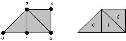
Figure 1: Simplicial mesh with enumerated vertices and simplices.

In addition to $\mathbb{V}$ and $\mathbb{S}_{n}$, an $n$-dimensional simplicial complex is comprised by its $p$-dimensional faces, $\mathbb{S}_{p},0\leq p<n$. In the case of Figure 1, these are

$$\mathbb{S}_{0}=\begin{bmatrix}0\\ 1\\ 2\\ 3\\ 4\end{bmatrix}, \mathbb{S}_{1}=\begin{bmatrix}0&1\\ 0&3\\ 1&2\\ 1&3\\ 2&3\\ 2&4\\ 3&4\end{bmatrix},$$

which correspond to the vertices (0-simplices) and oriented edges (1-simplices) of the complex. A graphical representation of this simplicial complex is shown in Figure 2. Since the orientation of the lower ($<n$) dimensional faces is arbitrary, we use the convention that face indices will be in sorted order. Furthermore, we require the rows of $\mathbb{S}$ to be sorted in lexicographical order. As pointed out in Section 7 and 9, these conventions facilitate efficient construction of differential operators and stiffness matrices.

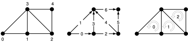
Figure 2: Simplicial complex with oriented edges and triangles.

4 Regular Cube Complex Representation

PyDEC provides a regular cube complex of dimension $n$ embedded in $\mathbb{R}^{n}$ for any $n$. As mentioned earlier, in dimension higher than 3, constructing simplicial manifold complexes is hard. In fact, even construction of good tetrahedral meshes is still an active area in computational geometry. This is one reason for using regular cube complexes in high dimensions. Moreover, for some applications, like topological image analysis or analysis of voxel data, the regular cube complex is a very convenient framework [39].

A regular cube complex can be easily specified by an $n$-dimensional array of binary values (bitmap) and a regular $n$-dimensional cube is placed where the bit is on. For example the cube complex shown in Figure 3 can be created by specifying the bitmap array

$$\begin{bmatrix}0&1\\ 1&1\end{bmatrix}\,.$$

A bitmap suffices to describe the top level cubes, but a cube array (like simplex array) is used during construction of differential operators and for computing faces. In this paper we describe the construction of exterior derivative, Hodge star and Whitney forms on simplicial complexes. For cube complexes we describe only the construction of exterior derivative and lower dimensional faces. However, the other operators and objects are also implemented in PyDEC for such complexes. For example, Whitney-like elements for hexahedral grids are described in [11] and are implemented in PyDEC.

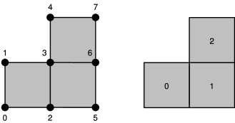
Figure 3: Regular cube mesh with enumerated vertices and faces.

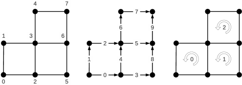
Figure 4: Regular cube complex with oriented edges and faces.

Converting a bitmap representation of a mesh into a cube array representation is straightforward. For example, the cube array representation of the mesh in Figure 3 is

$$\mathbb{C}_{2}=\begin{bmatrix}0&0&&0&1\\ 1&0&&0&1\\ 1&1&&0&1\end{bmatrix}.$$

As with the simplex arrays, the rows of $\mathbb{C}_{2}$ correspond to individual two-dimensional cubes in the mesh. The two left-most columns of $\mathbb{C}_{2}$ encode the origins of each two-dimensional cube, namely $(0,0)$, $(1,0)$ and $(1,1)$. The remaining two columns encode the coordinate directions spanned by the cube. Since $\mathbb{C}_{2}$ represents the top-level elements, all cubes span both the $x$ (coordinate $0$) and $y$ (coordinate $1$) dimensions. In general, the first $n$ columns of $\mathbb{C}_{k}$ encode the origin or corner of a cube while the remaining $k$ columns identify the coordinate directions swept out by the cube. We note that the cube array representation is similar to the cubical notation used by Sen [49].

The edges of the mesh in Figure 3 are represented by the cube array

$$\mathbb{C}_{1}=\begin{bmatrix}0&0&&0\\ 0&0&&1\\ 0&1&&0\\ 1&0&&0\\ 1&0&&1\\ 1&1&&0\\ 1&1&&1\\ 1&2&&0\\ 2&0&&1\\ 2&1&&1\end{bmatrix}\,$$

where again the first two columns encode the origin of each edge and the last column indicates whether the edge points in the $x$ or $y$ direction. For example, the row $[0,0,0]$ corresponds to edge $0$ in Figure 4 which begins at $(0,0)$ and extends one unit in the $x$ direction. Similarly the row $[2,1,1]$ encodes an edge starting at $(2,1)$ extending one unit in the $y$ direction. Since zero-dimensional cubes (points) have no spatial extent their cube array representation

$$\mathbb{C}_{0}=\begin{bmatrix}0&0\\ 0&1\\ 1&0\\ 1&1\\ 1&2\\ 2&0\\ 2&1\\ 2&2\\ \end{bmatrix}\,$$

contains only their coordinate locations.

The cube array provides a convenient representation for regular cube complexes. While a bitmap representation of the top-level cubes is generally more compact, the cube array representation generalizes naturally to lower-dimensional faces and is straightforward to manipulate.

5 Rips Complex Representation

The Rips complex, or Vietoris-Rips complex of a point set is defined by forming a simplex for every subset of vertices with diameter less than or equal to a given distance $r$. For example, if pair of vertices $(v_{i},v_{j})$ are no more than distance $r$ apart, then the Rips complex contains an edge (1-simplex) between the vertices. In general, a set of $p\geq 2$ vertices forms a $(p-1)$-simplex when all pairs of vertices in the set are separated by at most $r$.

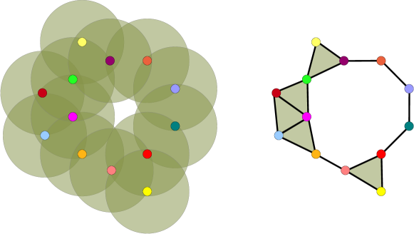
Figure 5: Broadcast radii and Rips complex for a sensor network.

In recent work, certain sensor network coverage problems have been shown to reduce to finding topological properties of the network’s Rips complex, at least for an abstract model of sensor networks [17]. Such coordinate-free methods rely only on pairwise communication between nodes and do not require the use of positioning devices. These traits are especially important in the context of ad-hoc wireless networks with limited per-node resources. Figure 5 depicts a planar sensor network and its associated Rips complex.

In this section we describe an efficient method for computing the Rips complex for a set of points. Although we consider only the case of points embedded in Euclidean space, our methodology applies to more general metric spaces. Indeed, only the construction of the $1$-skeleton of the Rips complex requires metric information. The higher-dimensional simplices are constructed directly from the $1$-skeleton.

We compute the $1$-skeleton of the Rips complex with a kD-Tree data structure. Specifically, for each vertex $v_{i}$ we compute the set of neighboring vertices $\{v_{j}:\lVert v_{j}-v_{i}\rVert\leq r\}$. The hierarchical structure of the kD-Tree allows such queries to be computed efficiently.

The $1$-skeleton of the Rips complex is stored in an array $\mathbb{S}_{1}$, using the convention discussed in Section 3. Additionally, the (oriented) edges of the $1$-skeleton are used to define $\mathbb{E}$, a directed graph stored in a sparse matrix format. Specifically, $\mathbb{E}(i,j)=1$ if $[i,j]$ is an edge of the Rips complex, and zero otherwise. For the Rips complex depicted in Figure 6,

$$\mathbb{S}_{1}=\begin{bmatrix}0&1\\ 0&2\\ 0&3\\ 1&3\\ 2&3\end{bmatrix}, \mathbb{E}=\begin{bmatrix}0&1&1&1\\ 0&0&0&1\\ 0&0&0&1\\ 0&0&0&0\end{bmatrix},$$

are the corresponding simplex array and directed graph respectively.

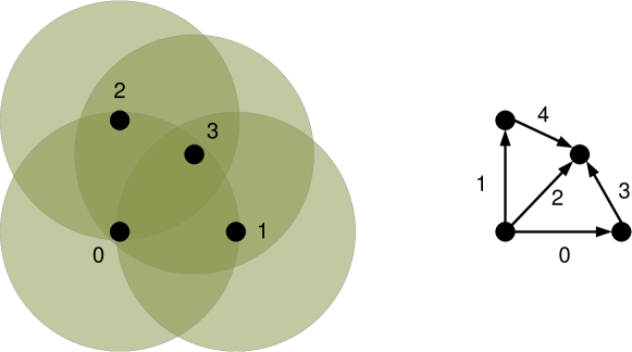
Figure 6: Five directed edges form the $1$-skeleton of the Rips complex.

The arrays of higher dimensional simplices $\mathbb{S}_{2},\mathbb{S}_{3},\ldots$ can be computed as follows. Let $\mathbb{F}_{p}$ denote the (sparse) matrix whose rows are identified with the $p$-simplices as specified by $\mathbb{S}_{p}$. Each row of $\mathbb{F}_{p}$ encodes the vertices which form the corresponding simplex. Specifically, $\mathbb{F}_{p}(i,j)$ takes the value $1$ if the $i$-th simplex contains vertex $j$ and zero otherwise. For the example shown in Figure 6,

$$\mathbb{F}_{1}=\begin{bmatrix}1&1&0&0\\ 1&0&1&0\\ 1&0&0&1\\ 0&1&0&1\\ 0&0&1&1\end{bmatrix},$$

encodes the edges stored in $\mathbb{S}_{1}$. Once $\mathbb{F}_{p}$ is constructed we compute the sparse matrix-matrix product $\mathbb{F}_{p}\,\mathbb{E}$. For our example the result is

$$\mathbb{F}_{1}\,\mathbb{E}=\begin{bmatrix}0&1&1&2\\ 0&1&1&2\\ 0&1&1&1\\ 0&0&0&1\\ 0&0&0&1\end{bmatrix}.$$

Like $\mathbb{F}_{p}$, the product $\mathbb{F}_{p}\,\mathbb{E}$ is a matrix that relates the $p$-simplices to the vertices: the matrix entry $(i,j)$ of $\mathbb{F}_{p}\,\mathbb{E}$ counts the number of directed edges that exist from the vertices of simplex $i$ to vertex $j$. When the value of $(i,j)$ entry of $\mathbb{F}_{p}\,\mathbb{E}$ is equal to $p+1$, we form a $p$-simplex of the Rips complex by concatenating simplex $i$ with vertex $j$. In the example, matrix entries $(0,3)$ and $(1,3)$ of $\mathbb{F}_{1}\,\mathbb{E}$ are equal to $2$ which implies that the $2$-skeleton of the Rips complex contains two simplices, formed by appending vertex $3$ to the $1$-simplices $[0,1]$ and $[0,2]$, or

$$\mathbb{S}_{2}=\begin{bmatrix}0&1&3\\ 0&2&3\end{bmatrix},$$

in array format. This process may be applied recursively to develop higher dimensional simplices $\mathbb{S}_{3},\mathbb{S}_{4},\ldots$ as required by the application. Thus our algorithm computes simplices of the Rips complex with a handful of sparse and dense matrix operations.

6 Abstract Simplicial Complex Representation

In Section 5 we saw an example of a simplicial complex which was not a manifold complex (Figure 5). Rips complexes described in Section 5 demonstrate one way to construct such complexes in PyDEC, starting from locations of vertices. There are other applications, for example in topology, where we would like to create a simplicial complex which is not necessarily a manifold. In addition we would like to do this without requiring that the location of vertices be given. For example, in topology, surfaces are often represented as a polygon with certain sides identified. One way to describe such an object is as an abstract simplicial complex [45, Section 3]. This is a collection of finite nonempty sets such that if a set is in the collection, so are all the nonempty subsets of it. Figure 7 shows two examples of abstract simplicial complexes created in PyDEC.

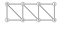
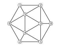
Figure 7: Examples of abstract simplicial complexes. The one of the left represents the triangulation of a Möbius strip and the one on the right that of a projective plane.

In PyDEC, abstract simplicial complexes are created by specifying a list of arrays. Each array contains simplices of a single dimension, specified as an array of vertex numbers. Lower dimensional faces of a simplex need not be specified explicitly. For example the Möbius strip triangulation shown in Figure 7 can be created by giving the array

$$\begin{bmatrix}0&1&3\\ 0&3&5\\ 3&2&5\\ 5&2&4\\ 2&0&4\\ 0&1&4\end{bmatrix}$$

as input to PyDEC. Abstract simplicial complexes need not be a triangulation of a manifold. For example one consisting of 2 triangles with an extra edge attached and a standalone vertex may be created using a list consisting of the arrays

$$\begin{bmatrix}5\end{bmatrix}\qquad\begin{bmatrix}1&4\end{bmatrix}\qquad\begin{bmatrix}0&1&2\\ 1&2&3\end{bmatrix}$$

as input.

The boundary matrices of a simplicial complex encode the connectivity information and can be computed from a purely combinatorial description of a simplicial complex. The locations of the vertices are not required. Thus the abstract simplicial complex structure is all that is required to compute these matrices as will be described in the next section.

7 Discrete Exterior Derivative

Given a manifold $M$, the exterior derivative $\operatorname{d}:\Omega^{p}(M)\to\Omega^{p+1}$ which acts on differential $p$-forms, generalizes the derivative operator of calculus. When combined with metric dependent operators Hodge star, sharp, and flat appropriately, the vector calculus operators div, grad and curl can be generated from $\operatorname{d}$. But $\operatorname{d}$ itself is a metric independent operators whose definition does not require any Riemannian metric on the manifold. See [1] for details. The discrete exterior derivative (which we will also denote as $\operatorname{d}$) in PyDEC is defined as is usual in the literature, as the coboundary operator of algebraic topology [45]. Thus

$$\langle\operatorname{d}_{p}a,c\rangle=\langle a,\operatorname{\partial}_{p+1}c\rangle\,,$$

for arbitrary $p$-cochain $a$ and $(p+1)$-chain $c$. Recall that the boundary operator on cochains, $\operatorname{\partial}_{p}:C_{p}(K)\to C_{p-1}(K)$ is defined by extension of its definition on an oriented simplex. The boundary operator on a $p$-simplex $\sigma^{p}=[v_{0},\ldots,v_{p}]$ is given in terms of its $(p-1)$-dimensional faces ($p+1$ in number) as

$$\operatorname{\partial}_{p}\sigma^{p}=\sum_{i=0}^{p}(-1)^{i}\bigl{[}v_{0},\ldots,\widehat{v_{i}},\ldots,v_{p}\bigr{]}\,,$$ (7.1)

where $\widehat{v_{i}}$ means that $v_{i}$ is omitted. Therefore, given an $n$-dimensional simplicial complex represented by $\mathbb{S}_{0},\dots,\mathbb{S}_{n}$, for the discrete exterior derivative, it suffices to compute $\operatorname{\partial}_{0},\dots,\operatorname{\partial}_{n}$. As is usual in algebraic topology, in PyDEC we compute matrix representations of these in the elementary chain basis. Boundary matrices are useful in finite elements since their transposes are the coboundary operators. They are also useful in computational topology since homology and cohomology groups are the quotient groups of kernel and image of boundary matrices [45].

For the complex pictured in Figure 2 the boundary operators are

$$\operatorname{\partial}_{0}=\begin{bmatrix}0&0&0&0&0\end{bmatrix}\,, \operatorname{\partial}_{1}=\begin{bmatrix}-1&-1&\phantom{-}0&\phantom{-}0&\phantom{-}0&\phantom{-}0&\phantom{-}0\\ \phantom{-}1&\phantom{-}0&-1&-1&\phantom{-}0&\phantom{-}0&\phantom{-}0\\ \phantom{-}0&\phantom{-}0&\phantom{-}1&\phantom{-}0&-1&-1&\phantom{-}0\\ \phantom{-}0&\phantom{-}1&\phantom{-}0&\phantom{-}1&\phantom{-}1&\phantom{-}0&-1\\ \phantom{-}0&\phantom{-}0&\phantom{-}0&\phantom{-}0&\phantom{-}0&\phantom{-}1&\phantom{-}1\end{bmatrix}\,,$$

$$\operatorname{\partial}_{2}=\begin{bmatrix}\phantom{-}1&\phantom{-}0&\phantom{-}0\\ -1&\phantom{-}0&\phantom{-}0\\ \phantom{-}0&\phantom{-}1&\phantom{-}0\\ \phantom{-}1&-1&\phantom{-}0\\ \phantom{-}0&\phantom{-}1&-1\\ \phantom{-}0&\phantom{-}0&\phantom{-}1\\ \phantom{-}0&\phantom{-}0&-1\end{bmatrix}.$$

In the following we describe an algorithm that takes as input $\mathbb{S}_{n}$ and computes both $\mathbb{S}_{n-1}$ and $\operatorname{\partial}_{n-1}$. This procedure is applied recursively to produce all faces of the complex and their boundary operator at that dimension.

The first step of the algorithm converts a simplex array $\mathbb{S}_{n}$ into a canonical format. In the canonical format each simplex (row of $\mathbb{S}_{n}$) is replaced by the simplex with sorted indices and the relative parity of the original ordering to the sorted order. For instance, the simplex $(1,3,2)$ becomes $((1,2,3),-1)$ since an odd number of transpositions (namely one) are needed to transform $(1,3,2)$ into $(1,2,3)$. Similarly, the canonical format for simplex $(2,1,4,3)$ is $((1,2,3,4),+1)$ since an even number of transpositions are required to sort the simplex indices. Since the complex dimension $n$ is typically small (i.e. $<10$), a simple sorting algorithm such as insertion sort is employed at this stage. We denote the aforementioned process canonical_format $(\mathbb{S}_{n})\to\mathbb{S}^{+}_{n}$ where the rightmost column of $\mathbb{S}^{+}_{n}$ contains the simplex parity. Applying canonical_format to $\mathbb{S}_{2}$ in our example yields

$$\mathbb{S}_{2}=\begin{bmatrix}0&1&3\\ 1&2&3\\ 2&4&3\end{bmatrix}\to\begin{bmatrix}0&1&3&&\phantom{-}1\\ 1&2&3&&\phantom{-}1\\ 2&3&4&&-1\end{bmatrix}=\mathbb{S}^{+}_{2}$$

Once a simplex array $\mathbb{S}_{n}$ has been transformed into canonical format, the $(n-1)$-dimensional faces $\mathbb{S}_{n-1}$ and boundary operator $\operatorname{\partial}_{n}$ are readily obtained. We denote this process

$$\texttt{boundary\_faces}(\mathbb{S}^{+}_{n})\to\mathbb{S}_{n-1},\operatorname{\partial}_{n}\,.$$

In order to establish the correspondence between the $n$-dimensional simplices and their faces, we first enumerate the simplices by adding another column to $\mathbb{S}^{+}_{n}$ to form $\mathbb{S}^{++}_{n}$. For example,

$$\mathbb{S}^{+}_{2}=\begin{bmatrix}0&1&3&&\phantom{-}1\\ 1&2&3&&\phantom{-}1\\ 2&3&4&&-1\end{bmatrix}\to\mathbb{S}^{++}_{2}=\begin{bmatrix}0&1&3&&\phantom{-}1&&0\\ 1&2&3&&\phantom{-}1&&1\\ 2&3&4&&-1&&2\end{bmatrix}.$$

The formula (7.1) is applied to $\mathbb{S}^{++}_{n}$ in a columnwise fashion by excluding the $i$-th column of simplex indices, multiplying the parity column by $(-1)^{i}$, and carrying the last column over unchanged. For example,

$$\mathbb{S}^{++}_{2}=\begin{bmatrix}0&1&3&&\phantom{-}1&&0\\ 1&2&3&&\phantom{-}1&&1\\ 2&3&4&&-1&&2\end{bmatrix}\to\begin{bmatrix}1&3&&\phantom{-}1&&0\\ 2&3&&\phantom{-}1&&1\\ 3&4&&-1&&2\\ 0&3&&-1&&0\\ 1&3&&-1&&1\\ 2&4&&\phantom{-}1&&2\\ 0&1&&\phantom{-}1&&0\\ 1&2&&\phantom{-}1&&1\\ 2&3&&-1&&2\end{bmatrix}$$

The resultant array is then sorted by the first $n$ columns in lexicographical order, allowing the unique faces to then be extracted.

$$\begin{bmatrix}1&3&&\phantom{-}1&&0\\ 2&3&&\phantom{-}1&&1\\ 3&4&&-1&&2\\ 0&3&&-1&&0\\ 1&3&&-1&&1\\ 2&4&&\phantom{-}1&&2\\ 0&1&&\phantom{-}1&&0\\ 1&2&&\phantom{-}1&&1\\ 2&3&&-1&&2\end{bmatrix}\to\begin{bmatrix}0&1&&\phantom{-}1&&0\\ 0&3&&-1&&0\\ 1&2&&\phantom{-}1&&1\\ 1&3&&\phantom{-}1&&0\\ 1&3&&-1&&1\\ 2&3&&\phantom{-}1&&1\\ 2&3&&-1&&2\\ 2&4&&\phantom{-}1&&2\\ 3&4&&-1&&2\\ \end{bmatrix}\to\begin{bmatrix}0&1\\ 0&3\\ 1&2\\ 1&3\\ 2&3\\ 2&4\\ 3&4\\ \end{bmatrix}.$$

Furthermore, a Compressed Sparse Row (CSR) [48] sparse matrix representation of $\operatorname{\partial}_{n}$ as

$$\operatorname{\partial}_{n}=(\texttt{ptr},\texttt{indices},\texttt{data})$$

is obtained from the sorted matrix. For $\operatorname{\partial}_{2}$ these are

ptr $$=\begin{bmatrix}0&1&2&3&5&7&8&9\end{bmatrix}\,,$$

indices $$=\begin{bmatrix}\phantom{-}0&\phantom{-}0&\phantom{-}1&\phantom{-}0&\phantom{-}1&\phantom{-}1&\phantom{-}2&\phantom{-}2&\phantom{-}2\end{bmatrix}\,,$$

data $$=\begin{bmatrix}\phantom{-}1&-1&\phantom{-}1&\phantom{-}1&-1&\phantom{-}1&-1&\phantom{-}1&-1\end{bmatrix}\,$$

where indices and data correspond to the fourth and third rows of the sorted matrix.

This process is then applied to $\mathbb{S}_{n-1}$ and so on down the dimension. Since the lower dimensional simplex array rows are already sorted, those arrays are already in canonical format. Thus a single algorithm generates the lower dimensional faces as well as the boundary matrices at all the dimensions. The boundary matrices, and hence the coboundary operators, are generated in a convenient sparse matrix format.

7.1 Generalization to Abstract Complexes

The boundary operators and faces of an abstract simplicial complex are computed with a straightforward extension of the boundary_faces algorithm. Recall from Section 6 that an abstract simplicial complex is specified by a list of simplex arrays of different dimensions, where the lower-dimensional simplex arrays represent simplices that are not a face of any higher-dimensional simplex. Generalizing the previous scheme to the case of abstract simplicial complexes is accomplished by (1) augmenting the set of computed faces with the user-specified simplices and (2) modifying the computed boundary operator accordingly.

Consider the abstract simplicial complex represented by the simplex arrays

$$\mathbb{S}_{0}=[5]\qquad\qquad\mathbb{S}_{1}=[1,4]\qquad\qquad\mathbb{S}_{2}=\begin{bmatrix}0&1&2\\ 1&2&3\end{bmatrix}$$

which consists of two triangles, an edge, and an isolated vertex. Applying boundary_faces to $\mathbb{S}_{2}$ produces an array of face edges and corresponding boundary operator

$$\texttt{boundary\_faces}(\mathbb{S}_{2})\to\mathbb{S}_{1},\operatorname{\partial}_{2}\ =\begin{bmatrix}0&1\\ 0&2\\ 1&2\\ 1&3\\ 2&3\\ \end{bmatrix},\begin{bmatrix}\phantom{-}1&\phantom{-}0\\ -1&\phantom{-}0\\ \phantom{-}1&\phantom{-}1\\ \phantom{-}0&-1\\ \phantom{-}0&\phantom{-}1\\ \end{bmatrix},$$

which includes all but the user-specified edge $[1,4]$. User-specified simplices are then incorporated into the simplex array in a three-stage process: (1) user-specified simplices are concatenated to the computed face array; (2) the rows of the combined simplex array are sorted lexicographically; (3) redundant simplices (if any) are removed from the sorted array. Upon completion, the augmented simplex array contains the union of the face simplices and the user-specified simplices. Continuing the example, the edge $[1,4]$ is incorporated into $\mathbb{S}_{1}$ as follows

$$\begin{bmatrix}0&1\\ 0&2\\ 1&2\\ 1&3\\ 2&3\\ \end{bmatrix},\begin{bmatrix}1&4\\ \end{bmatrix}\to\begin{bmatrix}0&1\\ 0&2\\ 1&2\\ 1&3\\ 2&3\\ 1&4\\ \end{bmatrix}\to\begin{bmatrix}0&1\\ 0&2\\ 1&2\\ 1&3\\ 1&4\\ 2&3\\ \end{bmatrix}\to\begin{bmatrix}0&1\\ 0&2\\ 1&2\\ 1&3\\ 1&4\\ 2&3\\ \end{bmatrix}=\mathbb{S}_{1}$$

In the final stage of the procedure, the computed boundary operator ($\operatorname{\partial}_{2}$ in the example) is updated to reflect the newly incorporated simplices. Since the new simplices do not lie in the boundary of any higher-dimensional simplex, we may simply add empty rows into the sparse matrix representation of the boundary operator for each newly added simplex. Therefore, the boundary operator update procedure amounts to a simple remapping of row indices. In the example, the addition of the edge $[1,4]$ into the fifth row of the simplex array requires the addition of an empty row into the boundary operator at the corresponding position,

$$\begin{bmatrix}\phantom{-}1&\phantom{-}0\\ -1&\phantom{-}0\\ \phantom{-}1&\phantom{-}1\\ \phantom{-}0&-1\\ \phantom{-}0&\phantom{-}1\\ \end{bmatrix}\to\begin{bmatrix}\phantom{-}1&\phantom{-}0\\ -1&\phantom{-}0\\ \phantom{-}1&\phantom{-}1\\ \phantom{-}0&-1\\ \phantom{-}0&\phantom{-}0\\ \phantom{-}0&\phantom{-}1\\ \end{bmatrix}=\operatorname{\partial}_{2}.$$

The Rips complex of Section 5 does have the location information for the vertices. However, ignoring those, such a complex is an abstract simplicial complex. Thus the boundary matrices for a Rips complex can be computed as described above. In practice some efficiency can be obtained by ordering the computation differently, so that the matrices are built as the complex is being built from the edge skeleton of the Rips complex. That is how it is implemented in PyDEC.

7.2 Boundary operators and faces for cubical complexes

The algorithm used to compute the faces and boundary operator of a given cube array ($\mathbb{C}_{p}\rightarrow\mathbb{C}_{p-1},\operatorname{\partial}_{p}$) is closely related to the procedure discussed in Section 7 for simplex arrays. Consider a general $p$-cube in $n$-dimensions, denoted by the pair $\bigl{[}(c_{0},\ldots,c_{n-1})(d_{0},\ldots,d_{p-1})\bigr{]}$ where $(c_{0},\ldots,c_{n-1})$ are the coordinates of cube’s origin and $(d_{0},\ldots,d_{p-1})$ are the directions which the $p$-cube spans. Note that the values $[c_{0},\ldots,c_{n-1},d_{0},\ldots,d_{p-1}]$ correspond exactly to a row of the cube array representation introduced in Section 4. Using this notation, the boundary of a $p$-cube is given by the expression

$$\operatorname{\partial}_{p}\bigl{[}(c_{0},\ldots,c_{n-1})(d_{0},\ldots,d_{p-1})\bigr{]}=\sum_{i=0}^{p-1}(-1)^{i}\bigl{(}\bigl{[}(c_{0},\ldots,c_{d_{i}}+1,\ldots,c_{n-1})(d_{0},\ldots,\widehat{d_{i}},\ldots,d_{p-1})\bigr{]}-\\ \bigl{[}(c_{0},\ldots,c_{d_{i}}+0,\ldots,c_{n-1})(d_{0},\ldots,\widehat{d_{i}},\ldots,d_{p-1})\bigr{]}\bigr{)}\,$$ (7.2)

where $\widehat{d_{i}}$ denotes the omission of the $i$-th spanning direction and $c_{d_{i}}$ is the corresponding coordinate. For example, the boundary of a square centered at the location $(10,20)$ is

$$\operatorname{\partial}_{2}\bigl{[}(10,20)(0,1)\bigr{]}=\bigl{[}(11,20)(1)\bigr{]}-\bigl{[}(10,20)(1)\bigr{]}-\bigl{[}(10,21)(0)\bigr{]}+\bigl{[}(10,20)(0)\bigr{]}.$$ (7.3)

The canonical format for a $p$-cube is the one where the spanning directions are specified in ascending order. For instance, the $2$-cube $\bigl{[}(10,20)(0,1)\bigr{]}$ is in the canonical format because $d_{0}<d_{1}$. As with simplices, each cube has a unique canonical format, through which duplicates are easily identified. Since the top-level cube array $\mathbb{C}_{n}$ is generated from a bitmap it is already in the canonical format and no reordering of indices or parity tracking is necessary.

Applying Equation 7.2 to a $p$-cube array with $N$ members generates a collection $2N$ oriented faces. In the mesh illustrated in Figure 3 the three squares in $\mathbb{C}_{2}$ are initially expanded into

$$\mathbb{C}_{2}=\begin{bmatrix}0&0&&0&1\\ 1&0&&0&1\\ 1&1&&0&1\end{bmatrix}\to\begin{bmatrix}0&0&&1&&-1&&0\\ 1&0&&1&&-1&&1\\ 1&1&&1&&-1&&2\\ 1&0&&1&&\phantom{-}1&&0\\ 2&0&&1&&\phantom{-}1&&1\\ 2&1&&1&&\phantom{-}1&&2\\ 0&0&&0&&\phantom{-}1&&0\\ 1&0&&0&&\phantom{-}1&&1\\ 1&1&&0&&\phantom{-}1&&2\\ 0&1&&0&&-1&&0\\ 1&1&&0&&-1&&1\\ 1&2&&0&&-1&&2\\ \end{bmatrix}=\mathbb{C}_{1}^{+}$$

where the fourth column of $\mathbb{C}_{1}^{+}$ encodes the orientation of the face and the fifth column records the $2$-cube to which each face belongs. Sorting the rows of $\mathbb{C}_{1}^{+}$ in lexicographical order

$$\begin{bmatrix}0&0&&1&&-1&&0\\ 1&0&&1&&-1&&1\\ 1&1&&1&&-1&&2\\ 1&0&&1&&\phantom{-}1&&0\\ 2&0&&1&&\phantom{-}1&&1\\ 2&1&&1&&\phantom{-}1&&2\\ 0&0&&0&&\phantom{-}1&&0\\ 1&0&&0&&\phantom{-}1&&1\\ 1&1&&0&&\phantom{-}1&&2\\ 0&1&&0&&-1&&0\\ 1&1&&0&&-1&&1\\ 1&2&&0&&-1&&2\\ \end{bmatrix}\to\begin{bmatrix}0&0&&0&\phantom{-}1&&0\\ 0&0&&1&-1&&0\\ 0&1&&0&-1&&0\\ 1&0&&0&\phantom{-}1&&1\\ 1&0&&1&-1&&1\\ 1&0&&1&\phantom{-}1&&0\\ 1&1&&0&\phantom{-}1&&2\\ 1&1&&0&-1&&1\\ 1&1&&1&-1&&2\\ 1&2&&0&-1&&2\\ 2&0&&1&\phantom{-}1&&1\\ 2&1&&1&\phantom{-}1&&2\\ \end{bmatrix}\to\begin{bmatrix}0&0&&0\\ 0&0&&1\\ 0&1&&0\\ 1&0&&0\\ 1&0&&1\\ 1&1&&0\\ 1&1&&1\\ 1&2&&0\\ 2&0&&1\\ 2&1&&1\end{bmatrix}=\mathbb{C}_{1}$$

allows the unique faces to be extracted. Lastly, a sparse matrix representation of the boundary operator is obtained from the sorted cube array in the same manner as for simplices.

8 Review of Whitney Map and Whitney Forms

In this section we review and collect some material, most of which is well-known in DEC and finite element exterior calculus research communities. It is included here partly to fix notation. In this section we also give the monomials based definition of inner product of differential forms. This is not the way inner product of forms is usually defined in most textbooks, [44] being one exception we know of. The monomial form leads to an efficient algorithm for computation of stiffness and mass matrices for Whitney forms given in Section 9.

The basic function spaces that are useful with exterior calculus are the space of square integrable $p$-forms on a manifold and Sobolev spaces derived from that. Let $M$ be a Riemannian manifold, a manifold on which a smoothly varying inner product is defined on the tangent space at each point. Let $g$ be its metric, a smooth tensor field that defines the inner product on the tangent space at each point on $M$.

For differential forms on such a manifold $M$, the space of square integrable forms is denoted $L^{2}\Omega^{p}(M)$. One can then define the spaces $H\Omega^{p}(M)$ which generalize the spaces $H(\operatorname{div})$ and $H(\operatorname{curl})$ used in mixed finite element methods [4]. To define $L^{2}\Omega^{p}(M)$ one has to define an inner product on the space of forms which is our starting point for this section. All these function spaces have been discussed in [2] and [4]. The definitions and properties of Whitney map and Whitney forms is in [21], the geometric analysis background is in [38] and the basic definition of inner products on forms is in [1, page 411].

8.1 Inner product of forms

To define the spaces $L^{2}\Omega^{p}(M)$ and $H\Omega^{p}(M)$ more precisely, we recall the definitions related to inner products of forms. We will need the exterior calculus operators wedge product and Hodge star which we recall first. For a manifold $M$ the wedge product $\wedge:\Omega^{p}(M)\times\Omega^{q}(M)\to\Omega^{p+q}(M)$ is an operator for building $(p+q)$-forms from $p$-forms and $q$-forms. It is defined as the skew-symmetrization of the tensor product of the two forms involved. For a Riemannian manifold of dimension $n$, the Hodge star operator $\operatorname{\ast}:\Omega^{p}(M)\to\Omega^{n-p}(M)$ is an isomorphism between the spaces of $p$ and $(n-p)$-forms. For more details, see [1, page 394] for wedge products and [1, page 411] for Hodge star.

Definition 8.1.

Given two smooth $p$-forms $\alpha$, $\beta\in\Omega^{p}(M)$ on a Riemannian manifold $M$, their pointwise inner product at point $x\in M$ is defined by

$$\langle\alpha(x),\beta(x)\rangle\,\mu=\alpha(x)\wedge\operatorname{\ast}\beta(x)\,,$$ (8.1)

where $\mu=\operatorname{\ast}1$ is the volume form associated with the metric induced by the inner product on $M$.

The pointwise inner products of forms can be defined in another way, which will be more useful to us in computations. The second definition given below in Definition 8.2 is equivalent to the one given above in Definition 8.1. The operator $\sharp$ (the sharp operator) used below is an isomorphism between 1-forms and vector fields and is defined by $g(\alpha^{\sharp},X)=\alpha(X)$ for given 1-form $\alpha$ and all vector fields $X$. See [1] for details.

Definition 8.2.

Let $\alpha_{1},\dots,\alpha_{p}$ and $\beta_{1},\dots,\beta_{p}$ be 1-forms on a Riemannian manifold $M$. By analogy with polynomials we’ll call $p$-forms of the type $\alpha_{1}\wedge\dots\wedge\alpha_{p}$ and $\beta_{1}\wedge\dots\wedge\beta_{p}$ monomial $p$-forms. Define the following operator at a point $x\in M$:

$$\bigl{\langle}\alpha_{1}\wedge\dots\wedge\alpha_{p},\beta_{1}\wedge\dots\wedge\beta_{p}\bigr{\rangle}:=\det\bigl{[}g\bigl{(}\alpha_{i}^{\sharp},\beta_{j}^{\sharp}\bigr{)}\bigr{]}\,,$$ (8.2)

where $\bigl{[}g\bigl{(}\alpha_{i}^{\sharp},\beta_{j}^{\sharp}\bigr{)}\bigr{]}$ is the matrix obtained by taking $1\leq i,j\leq p$. In the equation above, all the 1-forms are evaluated at the point $x\in M$. Extend the operation in (8.2) bilinearly pointwise to the space of all $p$-forms. It can be shown that this defines a pointwise inner product of $p$-forms equivalent to the one defined in (8.1). Note that if $\alpha_{i}=\beta_{i}$ for all $i$, the expression on the right in (8.2) is the Gram determinant.

Remark 8.3.

Note that unlike (8.1) the definition in (8.2) does not involve wedge product and Hodge star explicitly. This is an advantage of the latter form since a discrete wedge product is not available in PyDEC. The RHS of (8.2) does involve the sharp operator, but as we will see in the next section, this is easy to interpret for the purpose of discretization in this context.

Definition 8.4.

The pointwise innerproduct in (8.1), or equivalently in (8.2), induces an $L^{2}$ inner product on $M$ as

$$(\alpha,\beta)_{L^{2}}=\int_{M}\langle\alpha(x),\beta(x)\rangle\,\mu\,.$$ (8.3)

The space of $p$-forms obtained by completion of $\Omega^{p}(M)$ under this inner product is the Hilbert space of square integrable $p$-forms $L^{2}\Omega^{p}(M)$. The other useful space mentioned at the beginning of this section is the Sobolev space $H\Omega^{p}(M):=\{\alpha\in L^{2}\Omega^{p}(M)\;|\;\operatorname{d}\alpha\in L^{2}\Omega^{p+1}(M)\}$.

8.2 Whitney map and Whitney forms

Let $K$ be an $n$-dimensional manifold simplicial complex embedded in $\mathbb{R}^{N}$ and $\lvert K\rvert$ the underlying space. The metric on the interiors of the top dimensional simplices of $K$ will be the one induced from the embedding Euclidean space $\mathbb{R}^{N}$. As is usual in finite element methods, finite dimensional subspaces of the function spaces described in the previous paragraph are used in the numerical solution of PDEs. The finite dimensional spaces can be obtained by “embedding” the space of cochains into these spaces by using an interpolation. For example, to embed $C^{p}(K;\mathbb{R})$ into $L^{2}\Omega^{p}\bigl{(}\lvert K\rvert\bigr{)}$ one can use the Whitney map $\operatorname{W}:C^{p}(K;\mathbb{R})\to L^{2}\Omega^{p}\bigl{(}\lvert K\rvert\bigr{)}$, which will be reviewed in this subsection. The image $\operatorname{W}\bigl{(}C^{p}(K;\mathbb{R})\bigr{)}$ is a linear vector subspace of $L^{2}\Omega^{p}\bigl{(}\lvert K\rvert\bigr{)}$ and is the space of Whitney $p$-forms [52, 21, 13] and is denoted $\mathcal{P}_{1}^{-}\Omega^{p}(\lvert K\rvert)$ in [3, 4]. (We use $\Omega^{p}$ instead of $\Lambda^{p}$ used in [4].) The embedding of cochains is analogous to how scalar values at discrete sample points would be interpolated to get a piecewise affine function. In the scalar case also, the space of such functions is a vector subspace of square integrable functions. In fact, $\operatorname{W}\bigl{(}C^{0}(K;\mathbb{R})\bigr{)}$, the space of Whitney $0$-forms is the space of continuous piecewise affine functions on $\lvert K\rvert$. The Whitney map for $p>0$ is actually built from barycentric coordinates which are the building blocks of piecewise linear interpolation. Thus the embedding of $C^{p}(K;\mathbb{R})$ into $L^{2}\Omega^{p}\bigl{(}\lvert K\rvert\bigr{)}$ for $p>0$ can be considered to be a generalization of the embedding of $C^{0}(K;\mathbb{R})$ into $L^{2}\Omega^{0}\bigl{(}\lvert K\rvert\bigr{)}$. Thus Whitney forms enable only low order methods. However, arbitrary degree polynomial spaces suitable for use in finite element exterior calculus have been discovered [2, 3]. These however are not yet a part of PyDEC.

The space of Whitney $p$-forms is the space of piecewise smooth differential $p$-forms obtained by applying the Whitney map to $p$-cochains. It can be thought of as a method for interpolating values given on $p$-simplices of a simplicial complex. For example, inside a tetrahedron Whitney forms allow the interpolation of numbers on edges or faces to a smooth 1-form or 2-form respectively. As mentioned above, for 0-cochains, i.e. scalar functions sampled at vertices, the interpolation is the one obtained using the standard scalar piecewise affine basis functions on each simplex, that is the barycentric coordinates corresponding to each vertex of the simplex. We recall the definition of barycentric coordinates followed by the definition of the Whitney map.

Definition 8.5.

Let $\sigma^{p}=[v_{0},\ldots,v_{p}]$ be a $p$-simplex embedded in $\mathbb{R}^{N}$. The affine functions $\mu_{i}:\mathbb{R}^{N}\to\mathbb{R}$, $i=0,\ldots,p$, which when restricted to $\sigma^{p}$ take the value 1 on vertex $v_{i}$ and 0 on the others, are called the barycentric coordinates in $\sigma^{p}$.

Definition 8.6.

Let $\sigma^{p}$ be an oriented $p$-simplex $[v_{i_{0}},\ldots,v_{i_{p}}]$ in an $n$-dimensional manifold complex $K$, and $\bigl{(}\sigma^{p}\bigr{)}^{\ast}$ the corresponding elementary $p$-cochain. We define

$$\operatorname{W}\left(\left(\sigma^{p}\right)^{\ast}\right):=p!\sum_{k=0}^{p}(-1)^{k}\mu_{i_{k}}\,d\mu_{i_{0}}\wedge\cdots\wedge\widehat{d\mu_{i_{k}}}\wedge\cdots\wedge d\mu_{i_{p}}\,,$$ (8.4)

where $\mu_{i_{k}}$ is the barycentric coordinate function with respect to vertex $v_{i_{k}}$ and the notation $\widehat{d\mu_{i_{k}}}$ indicates that the term $d\mu_{i_{k}}$ is omitted from the wedge product. The Whitney map $\operatorname{W}:C^{p}(K;\mathbb{R})\to L^{2}\Omega^{p}\bigl{(}\lvert K\rvert\bigr{)}$ is the above map $\operatorname{W}$ extended to all of $C^{p}(K;\mathbb{R})$ by requiring that $\operatorname{W}$ be a linear map. $\operatorname{W}(\left(\sigma^{p}\right)^{\ast})$ is called the Whitney form corresponding to $\sigma^{p}$, and for a general cochain $c$, $\operatorname{W}(c)$ is called the Whitney form corresponding to $c$.

For example, the Whitney form corresponding to the edge $[v_{0},v_{1}]$ is $\operatorname{W}([v_{0},v_{1}]^{\ast})=\mu_{0}\operatorname{d}\mu_{1}-\mu_{1}\operatorname{d}\mu_{0}\,,$ and the Whitney form corresponding to the triangle $[v_{1},v_{2},v_{3}]$ in a tetrahedron $[v_{0},v_{1},v_{2},v_{3}]$ is

$$\operatorname{W}([v_{1},v_{2},v_{3}]^{\ast})=2\,(\mu_{1}\operatorname{d}\mu_{2}\wedge\operatorname{d}\mu_{3}-\mu_{2}\operatorname{d}\mu_{1}\wedge\operatorname{d}\mu_{3}+\mu_{3}\operatorname{d}\mu_{1}\wedge\operatorname{d}\mu_{2})\,.$$

Remark 8.7.

If we were using local coordinate charts on a manifold then at any point a $p$-form would be a linear combination of monomials. Note from (8.4) that the Whitney form $\operatorname{W}(\sigma^{\ast})$ is a sum of monomials with coefficients. Thus Whitney forms allow us to treat forms at a point as a linear combination of monomials even though we are not using local coordinate charts.

We emphasize again that this section was a review of known material. We have tried to present this material in a manner which makes it easier to explain the examples of Section 11 and the construction of mass matrix for Whitney forms described in the next section.

9 Whitney Inner Product of Cochains

Given a manifold simplicial complex $K$, an inner product between two $p$-cochains $a$ and $b$ can be defined by first embedding these cochains into $L^{2}\Omega^{p}\bigl{(}\lvert K\rvert\bigr{)}$ using Whitney map and then taking the $L^{2}$ inner product of the resulting Whitney forms [21].

Definition 9.1.

Given two $p$-cochains $a,b\in C^{p}(K;\mathbb{R})$, their Whitney inner product is defined by

$$(a,b):=(\operatorname{W}a,\operatorname{W}b)_{L^{2}}=\int_{\lvert K\rvert}\langle\operatorname{W}a,\operatorname{W}b\rangle\mu\,,$$ (9.1)

using the $L^{2}$ inner product on forms given in (8.3). The matrix for Whitney inner product of $p$-forms in the elementary $p$-cochain basis will be denoted $M_{p}$. That is, $M_{p}$ is a square matrix of order $N_{p}$ (the number of $p$-simplices in $K$) such that the entry in row $i$ and column $j$ is $M_{p}(i,j)=\bigl{(}(\sigma_{i}^{p})^{\ast},(\sigma_{j}^{p})^{\ast}\bigr{)}$, where $(\sigma_{i}^{p})^{\ast}$ and $(\sigma_{j}^{p})^{\ast}$ are the elementary $p$-cochains corresponding to the $p$-simplices $\sigma_{i}^{p}$ and $\sigma_{j}^{p}$ with index number $i$ and $j$ respectively.

The integral in (9.1) is the sum of integrals over each top dimensional simplex in $K$. Inside each such simplex the inner product of smooth forms applies since the Whitney form in each simplex is smooth all the way up to the boundary of the simplex. The interior of each top dimensional simplex is given an inner product that is induced from the standard inner product of the embedding space $\mathbb{R}^{N}$.

Remark 9.2.

Given cochains $a,b\in C^{p}(K;\mathbb{R})$ we will refer to their representations in the elementary cochain basis also as $a$ and $b$. Then the matrix representation of the Whitney inner product of $a$ and $b$ is $(a,b)=a^{T}M_{p}b$.

The inner product of cochains defined in this way is a key concept that connects exterior calculus to finite element methods and different choices of the inner product lead to different discretizations of exterior calculus. This is because the inner product matrix $M_{p}$ is the mass matrix of finite element methods based on Whitney forms. The details of the efficient computation of $M_{p}$ for any $p$ and $n$ will be given in Section 9.2 and 9.3.

Recall that for a Riemannian manifold $M$, if $\operatorname{\delta}_{p+1}:\Omega^{p+1}(M)\to\Omega^{p}(M)$ is the codifferential, then the Laplace-deRham operator on $p$-forms is $\operatorname{\Delta}_{p}:=\operatorname{d}_{p-1}\operatorname{\delta}_{p}+\operatorname{\delta}_{p+1}\operatorname{d}_{p}$. For a boundaryless $M$ the codifferential $\operatorname{\delta}_{p+1}$ is the adjoint of the exterior derivative $d_{p}$. In case $M$ has a boundary, we have instead that

$$(\operatorname{d}_{p}\alpha,\beta)=(a,\operatorname{\delta}_{p+1}\beta)+\int_{\partial M}\alpha\wedge\operatorname{\ast}\beta\,.$$ (9.2)

See [1, Exercise 7.5E] for a derivation of the above. Now consider Poisson’s equation $\operatorname{\Delta}_{p}u=f$ on $p$-forms defined on a $p$-dimensional simplicial manifold complex $K$. For simplicity, we’ll consider the weak form of this using smooth forms rather than Sobolev spaces of forms. See [2, 4] for a proper functional analytic treatment. We will also assume that the correct boundary conditions are satisfied, so that the boundary term in (9.2) is 0. In our simple treatment, the weak form of the Poisson’s equation is to find a $u\in\Omega^{p}(\lvert K\rvert)$ such that $(\operatorname{\delta}_{p}u,\operatorname{\delta}_{p}v)_{L^{2}}+(\operatorname{d}_{p}u,\operatorname{d}_{p}v)_{L^{2}}=(f,v)_{L^{2}}$. Thus it is clear that a Galerkin formulation using Whitney forms $\mathcal{P}_{1}^{-}\Omega^{p}$ will require the computation of a term like $(\operatorname{d}_{p}\operatorname{W}a,\operatorname{d}_{p}\operatorname{W}b)_{L^{2}}$ for cochains $a$ and $b$. By the commuting property of Whitney forms $\operatorname{d}_{p}W=W\operatorname{d}_{p}$ (where the second $\operatorname{d}_{p}$ is the coboundary operator on cochains) we have that the above inner product is equal to $(\operatorname{W}\operatorname{d}_{p}a,\operatorname{W}\operatorname{d}_{p}b)_{L^{2}}$. (See [21] for a proof of the commuting property.) Now, by definition of the Whitney inner product of cochains in (9.1) this is equal to $(\operatorname{d}_{p}a,\operatorname{d}_{p}b)$ in the inner product on $(p+1)$-cochains. The matrix form of this inner product can be obtained from the mass matrix $M_{p+1}$ as $\operatorname{d}_{p}^{T}\,M_{p+1}\,\operatorname{d}_{p}$. This is what we mean when we say that the stiffness matrix can be computed easily from the mass matrix. The term on the right in the weak form will use the mass matrix $M_{p}$. Since codifferential of Whitney forms is 0, the first term in the weak form has to be handled in another way, as described in [4].

Remark 9.3.

Exploiting the aforementioned commutativity of Whitney forms to compute the stiffness matrix represents a significant simplification to our software implementation. While computing the stiffness matrix directly from the definition is possible, it is a complex operation which requires considerable programmer effort, especially if the performance of the implementation is important. In contrast, our formulation requires no additional effort and has the performance of the underlying sparse matrix-matrix multiplication implementation, an optimized and natively-compiled routine. All of the complex indexing, considerations of relative orientation, mappings between faces and indices, etc. is reduced to a simple linear algebra expression. The lower dimensional faces are oriented lexicographically and the orientation information required in stiffness matrix assembly is implicit in the boundary matrices.

9.1 Computing barycentric differentials

Given that the Whitney form $\operatorname{W}(\sigma^{\ast})$ in (8.4) is built using wedges of differentials of barycentric coordinates, it is clear that the algorithm for computing an inner product of Whitney forms involves computation of the gradients or differentials of the barycentric coordinates. The following lemma shows how these are computed using simple linear algebra operations.

Lemma 9.4.

Let $\sigma^{p}=[v_{0},\ldots,v_{p}]$ be a $p$-simplex embedded in $\mathbb{R}^{N}$, $p\leq N$ where the vertices $v_{i}\in\mathbb{R}^{N}$ are given in some basis for $\mathbb{R}^{N}$. Let $X\in\mathbb{R}^{N\times p}$ be a matrix whose $j$-th column consists of the components of $\operatorname{d}\mu_{j}$ in the dual basis, for $j=1,\ldots,p$ . Let $V_{0}\in\mathbb{R}^{N\times p}$ be a matrix whose $j$-th column is $v_{j}-v_{0}$, for $j=1,\ldots,p$. Then $X^{T}=\bigl{(}V_{0}^{T}V_{0}\bigr{)}^{-1}V_{0}^{T}=V_{0}^{+}$, the pseudoinverse of $V_{0}$.

Proof.

Let $\zeta=[\mu_{1},\dots,\mu_{p}]^{T}$ be the vector of barycentric coordinates (other than $\mu_{0}$) with respect to $\sigma^{p}$, for a point $x=[x_{1},\dots,x_{N}]^{T}\in\mathbb{R}^{N}$. Then by definition of barycentric coordinates and simplices, $V_{0}\zeta=x-v_{0}$ is the linear least squares system for the barycentric coordinates. Thus $\zeta=V_{0}^{+}(x-v_{0})$ which implies that $\operatorname{d}\zeta=X^{T}=V_{0}^{+}$. ∎

Remark 9.5.

The use of normal equations in the solution of the least squares problem in the above proposition suffers from the well-known condition squaring problem. This is only likely to be a problem if the simplices are nearly degenerate. In that case one can just use an orthogonalization method to compute a QR factorization and use that to solve the least squares problem. Notice that in typical physical problems $V_{0}$ will typically be $2\times 2$, $3\times 2$ or $3\times 3$ matrix so any of these methods are easy to implement.

Once the components for $\operatorname{d}\mu_{i}$ have been obtained for $i=1,\dots,p$, the components of $\operatorname{d}\mu_{0}$ can be obtained by noting that $\operatorname{d}\mu_{0}+\cdots+\operatorname{d}\mu_{p}=0$ which follows from the fact that the barycentric coordinates sum to 1. Also note that the components of the gradients $\nabla\mu_{i}$ will be the same as those of $\operatorname{d}\mu_{i}$ if the standard metric of Euclidean space is used for the embedding space $\mathbb{R}^{N}$ which is the case in all of PyDEC.

9.2 Whitney inner product matrix

We will now use the inner product of forms in (8.2) and the cochains inner product defined in (9.1) to give a formula for the computation of $M_{p}$, the Whitney inner product matrix for $p$-cochains. We will also refer to this as the Whitney mass matrix.

Notation 9.6.

Given simplices $\sigma$ and $\tau$ the notation $\sigma\succeq\tau$ or $\tau\preceq\sigma$ means $\tau$ is a face of $\sigma$. Note that this means $\tau$ can be equal to $\sigma$ since any simplex is its own face. For proper inclusion we use $\tau\prec\sigma$ or $\sigma\succ\tau$ to indicate that $\tau$ is a proper face of $\sigma$. The use of this notation simplifies the expression of summations over various classes of simplices in a complex. For example, given two fixed $p$-simplices $\sigma_{i}^{p}$ and $\sigma_{j}^{p}$

$$\underset{\sigma^{n}\succeq\sigma^{p}_{i},\sigma^{p}_{j}}{\sum_{\sigma^{n}}}$$

is read as “sum over all $n$-simplices $\sigma^{n}$ which have $\sigma_{i}^{p}$ and $\sigma_{j}^{p}$ as faces” . Another notation used in the proof of the proposition below is the star of a simplex $\sigma$, written $\operatorname{St}(\sigma)$ (not to be confused with the dual star $\star\sigma$). This star $\operatorname{St}(\sigma)$ is the union of the interiors of all simplices of the complex that have $\sigma$ as a face. That includes $\sigma$ also. The closure of this open set is called the closed star and written $\operatorname{\overline{St}}{\sigma}$. This is the union of simplices that contain $\sigma$.

Proposition 9.7.

Let $\sigma_{i}^{p}=[v_{i_{0}},\dots,v_{i_{p}}]$ and $\sigma_{j}^{p}=[v_{j_{0}},\dots,v_{j_{p}}]$ be oriented $p$-simplices in an $n$-dimensional manifold simplicial complex $K$, with $0\leq p\leq n$. Then the row $i$, column $j$ entry of the Whitney inner product matrix $M_{p}$ is given by

$$M_{p}(i,j)=(p!)^{2}\underset{\sigma^{n}\succeq\sigma^{p}_{i},\sigma^{p}_{j}}{\sum_{\sigma^{n}}}\sum_{k,l=0}^{p}(-1)^{k+l}c_{kl}\int_{\sigma^{n}}\mu_{i_{k}}\mu_{j_{l}}\,\mu\,,$$

where $c_{kl}=1$ for $p=0$, and for $p>0$

$$c_{kl}=\det\begin{bmatrix}\bigl{\langle}\operatorname{d}\mu_{i_{0}},\operatorname{d}\mu_{j_{0}}\bigr{\rangle}&\dots&\widehat{\bigl{\langle}\operatorname{d}\mu_{i_{0}},\operatorname{d}\mu_{j_{l}}\bigr{\rangle}}&\dots&\bigl{\langle}\operatorname{d}\mu_{i_{0}},\operatorname{d}\mu_{j_{p}}\bigr{\rangle}\\ \vdots&&\vdots&&\vdots\\ \widehat{\bigl{\langle}\operatorname{d}\mu_{i_{k}},\operatorname{d}\mu_{j_{0}}\bigr{\rangle}}&\dots&\widehat{\bigl{\langle}\operatorname{d}\mu_{i_{k}},\operatorname{d}\mu_{j_{l}}\bigr{\rangle}}&\dots&\widehat{\bigl{\langle}\operatorname{d}\mu_{i_{k}},\operatorname{d}\mu_{j_{l}}\bigr{\rangle}}\\ \vdots&&\vdots&&\vdots\\ \bigl{\langle}\operatorname{d}\mu_{i_{p}},\operatorname{d}\mu_{j_{0}}\bigr{\rangle}&\dots&\widehat{\bigl{\langle}\operatorname{d}\mu_{i_{p}},\operatorname{d}\mu_{j_{l}}\bigr{\rangle}}&\dots&\bigl{\langle}\operatorname{d}\mu_{i_{p}},\operatorname{d}\mu_{j_{p}}\bigr{\rangle}\end{bmatrix}\,,$$

the hats indicating the deleted terms. Here $\mu$ is the volume form corresponding to the standard inner product in $\mathbb{R}^{N}$ and $\mu_{i_{k}}$ and $\mu_{j_{l}}$ are the barycentric coordinates corresponding to vertices $i_{k}$ and $j_{l}$.

Proof.

See Appendix. ∎

For the $p=n$ case a simpler formulation is given in Proposition 9.9. The above proposition shows that computation of the Whitney inner product matrix involves computations of inner products of differentials of barycentric coordinates. Since the only metric implemented in PyDEC is the standard one inherited from the embedding space $\mathbb{R}^{N}$,

$$\bigl{\langle}\operatorname{d}\mu_{i},\operatorname{d}\mu_{j}\bigr{\rangle}=g((\operatorname{d}\mu_{i})^{\sharp},(\operatorname{d}\mu_{j})^{\sharp})=\nabla\mu_{i}\cdot\nabla\mu_{j}\,.$$

Example 9.8.

Consider the simplicial complex corresponding to a tetrahedron $\sigma^{3}$ embedded in $\mathbb{R}^{3}$ for which we want to compute $M_{2}$, the Whitney inner product matrix for 2-cochains. Here $N=n=3$ and $p=2$ and $M_{2}$ is of order $N_{2}=4$, the number of triangles in the complex. Label the vertices as $0,1,2,3$. Then by PyDEC’s lexicographic numbering scheme, the edges numbered 0 to 5 are $[0,1]$, $[0,2]$, $[0,3]$, $[1,2]$, $[1,3]$, $[2,3]$ and the triangles numbered 0 to 3 are $[0,1,2]$, $[0,1,3]$, $[0,2,3]$, and $[1,2,3]$. We will describe the computation of the row 0, column 3 entry and the row 0, column 1 entry of $M_{2}$. The $(0,3)$ entry corresponds to the inner product of cochains $[v_{0},v_{1},v_{2}]^{\ast}$ and $[v_{1},v_{2},v_{3}]^{\ast}$ since, in the lexicographic ordering and naming convention of PyDEC these are $\sigma^{2}_{0}$ and $\sigma^{2}_{3}$ respectively. Thus we are computing

$$\bigl{(}\bigl{(}\sigma^{2}_{0}\bigr{)}^{\ast},\bigl{(}\sigma^{2}_{3}\bigr{)}^{\ast}\bigr{)}=\bigl{(}\operatorname{W}\bigl{(}\sigma^{2}_{0}\bigr{)}^{\ast},\operatorname{W}\bigl{(}\sigma^{2}_{3}\bigr{)}^{\ast}\bigr{)}_{L^{2}}\,.$$

The corresponding Whitney forms are

$$\operatorname{W}\bigl{(}\sigma^{2}_{0}\bigr{)}^{\ast} =2!\,\bigl{(}\mu_{0}\,\operatorname{d}\mu_{1}\wedge\operatorname{d}\mu_{2}-\mu_{1}\operatorname{d}\mu_{0}\wedge\operatorname{d}\mu_{2}+\mu_{2}\operatorname{d}\mu_{0}\wedge\operatorname{d}\mu_{1}\bigr{)}$$

$$\operatorname{W}\bigl{(}\sigma^{2}_{3}\bigr{)}^{\ast} =2!\,\bigl{(}\mu_{1}\,\operatorname{d}\mu_{2}\wedge\operatorname{d}\mu_{3}-\mu_{2}\operatorname{d}\mu_{1}\wedge\operatorname{d}\mu_{3}+\mu_{3}\operatorname{d}\mu_{1}\wedge\operatorname{d}\mu_{2}\bigr{)}\,.$$

Then $\bigl{(}\operatorname{W}\bigl{(}\sigma^{2}_{0}\bigr{)}^{\ast},\operatorname{W}\bigl{(}\sigma^{2}_{3}\bigr{)}^{\ast}\bigr{)}_{L^{2}}/(2!)^{2}$ is

$$\int_{\sigma^{3}}\mu_{0}\mu_{1}\bigl{\langle}\operatorname{d}\mu_{1}\wedge\operatorname{d}\mu_{2},\operatorname{d}\mu_{2}\wedge\operatorname{d}\mu_{3}\bigr{\rangle}\,\mu-\\ \int_{\sigma^{3}}\mu_{0}\mu_{2}\bigl{\langle}\operatorname{d}\mu_{1}\wedge\operatorname{d}\mu_{2},\operatorname{d}\mu_{1}\wedge\operatorname{d}\mu_{3}\bigr{\rangle}\,\mu+\dots\,,$$ (9.3)

where $\mu$ is just $\operatorname{d}x\,\wedge\,\operatorname{d}y\,\wedge\,\operatorname{d}z$, the standard volume form in $\mathbb{R}^{3}$. Each term like $\bigl{\langle}\operatorname{d}\mu_{1}\wedge\operatorname{d}\mu_{2},\operatorname{d}\mu_{2}\wedge\operatorname{d}\mu_{3}\bigr{\rangle}$ is

$$\det\begin{bmatrix}\langle\operatorname{d}\mu_{1},\operatorname{d}\mu_{2}\rangle&\langle\operatorname{d}\mu_{1},\operatorname{d}\mu_{3}\rangle\\ \langle\operatorname{d}\mu_{2},\operatorname{d}\mu_{2}\rangle&\langle\operatorname{d}\mu_{2},\operatorname{d}\mu_{3}\rangle\end{bmatrix}\,,$$

which in the notation of Prop. 9.7 is

$$\det\begin{bmatrix}\widehat{\langle\operatorname{d}\mu_{0},\operatorname{d}\mu_{1}\rangle}&\widehat{\langle\operatorname{d}\mu_{0},\operatorname{d}\mu_{2}\rangle}&\widehat{\langle\operatorname{d}\mu_{0},\operatorname{d}\mu_{3}\rangle}\\ \widehat{\langle\operatorname{d}\mu_{1},\operatorname{d}\mu_{1}\rangle}&\langle\operatorname{d}\mu_{1},\operatorname{d}\mu_{2}\rangle&\langle\operatorname{d}\mu_{1},\operatorname{d}\mu_{3}\rangle\\ \widehat{\langle\operatorname{d}\mu_{2},\operatorname{d}\mu_{1}\rangle}&\langle\operatorname{d}\mu_{2},\operatorname{d}\mu_{2}\rangle&\langle\operatorname{d}\mu_{2},\operatorname{d}\mu_{3}\rangle\end{bmatrix}\,.$$

Using a shorthand notation for matrices like above, the $2\times 2$ matrices whose determinants need to be computed for calculating the $(0,3)$ entry of $M_{2}$ are given below.

$$\begin{array}[]{ccc}\begin{bmatrix}\widehat{01}&\widehat{02}&\widehat{03}\\ \widehat{11}&12&13\\ \widehat{21}&22&23\end{bmatrix}&\begin{bmatrix}\widehat{02}&\widehat{01}&\widehat{03}\\ \widehat{12}&11&13\\ \widehat{22}&21&23\end{bmatrix}&\begin{bmatrix}\widehat{03}&\widehat{01}&\widehat{02}\\ \widehat{13}&11&12\\ \widehat{23}&21&22\end{bmatrix}\\ &&\\ \begin{bmatrix}\widehat{11}&\widehat{12}&\widehat{13}\\ \widehat{01}&02&03\\ \widehat{21}&22&23\end{bmatrix}&\begin{bmatrix}\widehat{12}&\widehat{11}&\widehat{13}\\ \widehat{02}&01&03\\ \widehat{22}&21&23\end{bmatrix}&\begin{bmatrix}\widehat{13}&\widehat{11}&\widehat{12}\\ \widehat{03}&01&02\\ \widehat{23}&21&22\end{bmatrix}\\ &&\\ \begin{bmatrix}\widehat{21}&\widehat{22}&\widehat{23}\\ \widehat{01}&02&03\\ \widehat{11}&12&13\end{bmatrix}&\begin{bmatrix}\widehat{22}&\widehat{21}&\widehat{23}\\ \widehat{02}&01&03\\ \widehat{12}&11&13\end{bmatrix}&\begin{bmatrix}\widehat{23}&\widehat{21}&\widehat{22}\\ \widehat{03}&01&02\\ \widehat{13}&11&12\end{bmatrix}\end{array}$$

Removing the deleted rows and columns the above matrices are given below as the actual $2\times 2$ matrices.

$$\begin{array}[]{ccc}\begin{bmatrix}12&13\\ 22&23\end{bmatrix}&\begin{bmatrix}11&13\\ 21&23\end{bmatrix}&\begin{bmatrix}11&12\\ 21&22\end{bmatrix}\\ &&\\ \begin{bmatrix}02&03\\ 22&23\end{bmatrix}&\begin{bmatrix}01&03\\ 21&23\end{bmatrix}&\begin{bmatrix}01&02\\ 21&22\end{bmatrix}\\ &&\\ \begin{bmatrix}02&03\\ 12&13\end{bmatrix}&\begin{bmatrix}01&03\\ 11&13\end{bmatrix}&\begin{bmatrix}01&02\\ 11&12\end{bmatrix}\end{array}$$ (9.4)

The $2\times 2$ matrices whose determinants are needed in computing $\bigl{(}\bigl{(}\sigma^{2}_{0}\bigr{)}^{\ast},\bigl{(}\sigma^{2}_{1}\bigr{)}^{\ast}\bigr{)}$, i.e., entry $(0,1)$ of $M_{2}$ are given below.

$$\begin{array}[]{ccc}\begin{bmatrix}11&13\\ 21&23\end{bmatrix}&\begin{bmatrix}10&13\\ 20&23\end{bmatrix}&\begin{bmatrix}10&11\\ 20&21\end{bmatrix}\\ &&\\ \begin{bmatrix}01&03\\ 21&23\end{bmatrix}&\begin{bmatrix}00&03\\ 20&23\end{bmatrix}&\begin{bmatrix}00&01\\ 20&21\end{bmatrix}\\ &&\\ \begin{bmatrix}01&03\\ 11&13\end{bmatrix}&\begin{bmatrix}00&03\\ 10&13\end{bmatrix}&\begin{bmatrix}00&01\\ 10&11\end{bmatrix}\end{array}$$ (9.5)

Recall that each number in these matrices is shorthand for an inner product of two barycentric differentials. For example, the entry 12 stands for $\bigl{\langle}\operatorname{d}\mu_{1},\operatorname{d}\mu_{2}\bigr{\rangle}=g((\operatorname{d}\mu_{1})^{\sharp},(\operatorname{d}\mu_{2})^{\sharp})=\nabla\mu_{1}\cdot\nabla\mu_{2}$.

Proposition 9.9.

For $p=n$, $M_{p}$ is a diagonal matrix with $M_{p}(i,i)=1/\lvert\sigma_{i}^{n}\rvert$, where $\lvert\sigma_{i}^{n}\rvert$ is the volume of the simplex.

Proof.

For any $n$-simplex $\sigma^{n}$, the Whitney form $\operatorname{W}(\sigma^{n})^{\ast}$ is 0 on other $n$-simplices and so $M_{p}$ is diagonal. Furthermore, it is a constant coefficient volume form on $\sigma^{n}$ with $\int_{\sigma^{n}}\operatorname{W}(\sigma^{n})^{\ast}=1$. See [21] for proofs of these properties. Thus it must be that $\operatorname{W}(\sigma^{n})^{\ast}=\mu/\lvert\sigma^{n}\rvert$ where $\mu$ is the volume form on the simplex. Thus

$$\bigl{\langle}\operatorname{W}(\sigma^{n})^{\ast},\operatorname{W}(\sigma^{n})^{\ast}\bigr{\rangle}\,\mu=\operatorname{W}(\sigma^{n})^{\ast}\wedge\operatorname{\ast}\operatorname{W}(\sigma^{n})^{\ast}=\frac{\mu}{\lvert\sigma^{n}\rvert^{2}}\,.$$

Thus $\bigl{(}\operatorname{W}(\sigma^{n})^{\ast},\operatorname{W}(\sigma^{n})^{\ast}\bigr{)}_{L^{2}}$ is $\int_{\sigma^{n}}\mu/\lvert\sigma^{n}\rvert^{2}$ which is $1/\lvert\sigma^{n}\rvert$. ∎

9.3 Algorithm for Whitney inner product matrix

We motivate our algorithm for Whitney mass matrix computation by making some observations about Example 9.8. The first, and obvious observation is that matrix $M_{p}$ is symmetric, being an inner product matrix. Thus only the diagonal entries and those above (or below) the diagonal need be computed. A more interesting efficiency comes from the structure of the entries of the matrix collections, such as ones shown in (9.4) and (9.5). Note that many entries repeat in the shorthand collection of matrices in (9.4) and (9.5). For example the entry 12 appears 4 times by itself in the matrix collection (9.4). Moreover, due to the symmetry of inner product, the entry 12 corresponds to the same result as the entry 21 and 21 appears 4 times as well. That entry also appears 4 times in the collection (9.5). Thus it is clear that a saving in computational time can be achieved by doing such calculations only once. That is, $\langle\operatorname{d}\mu_{1},\operatorname{d}\mu_{2}\rangle=\langle\operatorname{d}\mu_{2},\operatorname{d}\mu_{1}\rangle$ need only be computed once for the tetrahedron.

The determinants of all the matrices in a collection such as (9.4) are needed to plug into an expression like (9.3) to obtain a single entry (in this case row 0, column 3) of the Whitney inner product matrix for $p$-cochains ($p=2$ in this case), whose size ($4\times 4$ in this case) depends on the number of $p$-simplices in the simplicial complex. Thus reusing repeated inner products of barycentric differentials can add up to a substantial saving in computational expense when all the unique entries of $M_{p}$ are computed. These savings are quantified later in this subsection.

Another useful point to note in the example calculation is that the collection (9.5) of matrices can be obtained from the collection (9.4) by keeping the first digit in each entry same and making the substitutions $1\rightarrow 0$; $2\rightarrow 1$; and $3\rightarrow 3$ in the second digit. The first digits in the two collections are the same because both correspond to the triangle $\sigma^{2}_{0}$. The substitution above works for the second digit because $\sigma^{2}_{3}=[v_{1},v_{2},v_{3}]$ and $\sigma^{2}_{1}=[v_{0},v_{1},v_{3}]$. This suggests the use of a template simplex for creating a template collection of matrices whose determinants are needed. The actual instances of the collections can then be obtained by using the vertex numbers in a given simplex. This is another idea that is used in the algorithm implemented in PyDEC. The algorithm takes as input a manifold simplicial $n$-complex $K$, embedded in $\mathbb{R}^{N}$ and $0\leq p\leq n$. The output is $M_{p}$, an $N_{p}\times N_{p}$ matrix representation of inner product on $C^{p}(K;\mathbb{R})$ using elementary cochain basis. If a naive algorithm, which does not take into account the duplications in determinant calculations were to be used, the number of operations required in the mass matrix calculation are

$$N_{n}\times\dfrac{\dbinom{n+1}{p+1}^{2}+\dbinom{n+1}{p+1}}{2}\times\binom{n}{p}^{2}\times Np^{2}\times(O(p!)\text{ or }O(p^{3}))\,.$$

The last term is written as $O(p!)$ or $O(p^{3})$ because a determinant can be computed using the formula for determinant or by LU factorization. For low values of $p$ (i.e. $\leq$ about 5) the formula will likely be better.

According to the above formula, for example, for $n=3,p=2$, the number of determinants required in a naive implementation of mass matrix calculation would be

$$\dfrac{\dbinom{4}{3}^{2}+\dbinom{4}{3}}{2}\times\binom{3}{2}^{2}=10\times 9=90\,.$$

But there are only 21 unique determinants needed for $n=3,p=2$. Our algorithm computes the unique determinants first and the operation count is

$$N_{n}\times\dfrac{\dbinom{n+1}{p}^{2}+\dbinom{n+1}{p}}{2}\times Np^{2}\times(O(p!)\text{ or }O(p^{3}))\,.$$

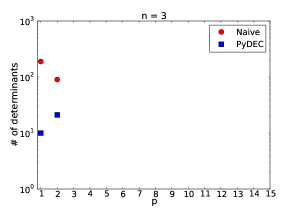
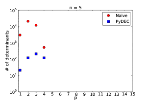
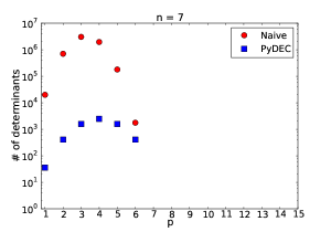
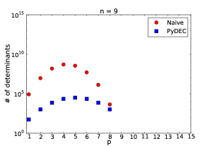
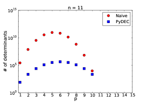
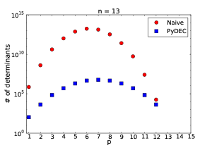
Figure 8: Comparison between PyDEC and a naive algorithm for computing Whitney mass matrix. The figure shows the number of determinant computations needed by the two algorithms, for various values of $p$, the Whitney form dimension, and $n$, the simplicial complex dimension. The embedding dimension is not relevant in these calculations. For $p=n$ case we use the shortcut described in Proposition 9.9 so that case is not shown.

Figure 8 shows a comparison of determinant counts for our algorithm compared with a naive algorithm that does the duplicate work that our PyDEC algorithm avoids. Note that for any $n$, the most advantage is gained intermediate values of $p$. The savings that the PyDEC implementation provides over a naive algorithm are several orders of magnitude, especially for moderately large $n$ and higher. For $p=n$ case, in PyDEC we use the shortcut described in Proposition 9.9.

10 Metric Dependent Operators

We now describe the PyDEC implementations of some metric dependent exterior calculus operators. The simplicial complex $K$ is now supposed to be an approximation of a Riemannian $n$-manifold $M$. The metric implemented in PyDEC is the one induced from an embedding space $\mathbb{R}^{N}$. The main metric dependent operator is the Hodge star which enables the discretization of codifferential and Laplace-deRham operators. The sharp and flat, which are isomorphisms between 1-forms and vector fields, are not implemented.

For the DEC Hodge star, the implementation is using the circumcentric dual as in [31, 19] and the other operators are then simply defined in terms of the exterior derivative and the Hodge star. For PyDEC’s implementation of low order finite element exterior calculus, we define the Hodge star to be the Whitney mass matrix described in Section 9. The other operators are defined by analogy with DEC even though the dual mesh concept is not part of finite element exterior calculus. Extensive experimental justification for this approach can be seen in its effectiveness in numerical experiments in [8] and in [32].

For the definitions in this section we will need two cochain complexes of real-valued cochains. One will be on the simplicial complex $K$ and for brevity we’ll call this space of $p$-cochains $C^{p}(K)$ instead of $C^{p}(K;\mathbb{R})$. The other cochain complex is on the circumcentric dual cell complex $\operatorname{\star}K$ and we’ll denote the $(n-p)$-dimensional cochains as $D^{n-p}(\operatorname{\star}K)$. At each dimension, these will be connected by discrete Hodge star operators to be defined below. Since the exterior derivative is the coboundary operator, the matrix representation for the exterior derivative on the dual mesh is the boundary operator. The matrix form for the DEC Hodge star on $p$-cochains will be denoted $\operatorname{\ast}_{p}:C^{p}(K)\to D^{n-p}(\operatorname{\star}K)$. One box of the primal and dual complexes is shown below.

$$\begin{CD}C^{p}(K)@>{\operatorname{d}_{p}}>{}>C^{p+1}(K)\\ @V{}V{\operatorname{\ast}_{p}}V@V{}V{\operatorname{\ast}_{p+1}}V\\ D^{n-p}(\operatorname{\star}K)@<{\operatorname{d}_{p}^{T}}<{}<D^{n-p-1}(\operatorname{\star}K)\end{CD}$$

As described in [31, 19] and other references, the DEC Hodge star is defined by

$$\frac{\langle\operatorname{\ast}_{p}\sigma^{\ast}_{i},\operatorname{\star}\sigma_{j}\rangle}{\lvert\operatorname{\star}\sigma_{j}\rvert}=\frac{\langle\sigma^{\ast}_{i},\sigma_{j}\rangle}{\lvert\sigma_{j}\rvert}\,,$$

for $p$-simplices $\sigma_{i}$ and $\sigma_{j}$. Here $\sigma^{\ast}$ is the elementary cochain corresponding to $\sigma$ and $\langle\sigma^{\ast},\tau\rangle$ stands for the evaluation of the cochain $\sigma^{\ast}$ on the elementary chain $\tau$. Thus the matrix representation of the DEC Hodge star $\operatorname{\ast}_{p}$ is as a diagonal matrix with $\operatorname{\ast}_{p}(i,i)=\lvert\operatorname{\star}\sigma_{i}\rvert/\lvert\sigma_{i}\rvert$. In [31, 19] this was defined for well-centered meshes. For the codimension 1 Hodge star the definition extends to Delaunay meshes with a slight additional condition for boundary simplices. This extension involves computing the volume of $\operatorname{\star}\sigma$ taking into account signs. Consider a codimension 1 simplex $\sigma$ shared by simplices $L$ and $R$. For the portion of $\operatorname{\star}\sigma$ corresponding to $L$, the sign is positive if the circumcenter and remaining vertex of $L$ are on the same side of $\sigma$. Similarly for $R$. (For surface meshes and higher dimensional analogs the circumcenter condition above is one way to define a Delaunay-like condition.) If $\sigma$ is a codimension 1 face of top dimensional $\tau$ and is on domain boundary then the circumcenter of $\tau$ and vertex opposite to $\sigma$ should be on the same side. The smooth Hodge star on $p$-forms satisfies $\operatorname{\ast}\operatorname{\ast}=(-1)^{p(n-p)}$. In the discrete setting $\operatorname{\ast}\operatorname{\ast}$ is written as $\operatorname{\ast}_{p}^{-1}\operatorname{\ast}_{p}$ or $\operatorname{\ast}_{p}\operatorname{\ast}_{p}^{-1}$ and this is defined to be $(-1)^{p(n-p)}\,I$ where $I$ is the identity matrix.

In the smooth theory, the codifferential $\operatorname{\delta}_{p+1}:\Omega^{p+1}(M)\to\Omega^{p}(M)$ is defined as $\operatorname{\delta}_{p+1}=(-1)^{np+1}\operatorname{\ast}\operatorname{d}\operatorname{\ast}$ and so we define the discrete codifferential $\operatorname{\delta}_{p+1}:C^{p}(K)\to C^{n-p}(K)$ as $\operatorname{\delta}_{p+1}:=(-1)^{np+1}\operatorname{\ast}_{p}^{-1}\operatorname{d}_{p}^{T}\operatorname{\ast}_{p+1}$. For finite element exterior calculus implemented in PyDEC, we take this to be the definition, without reference to a dual mesh. If we now take $\operatorname{\ast}_{p}$ to be the Whitney mass matrix then $\operatorname{d}_{p}$ and $\operatorname{\delta}_{p+1}$ are adjoints (up to sign) with respect to the Whitney inner product on cochains as shown in [32]. We will call the use of Whitney mass matrix as $\operatorname{\ast}_{p}$ to be a Whitney Hodge star matrix.

In the discrete setting the Laplace-deRham operator is implemented in the weak form. For $0<p<n$ the discrete definition is $\operatorname{\Delta}_{p}:=\operatorname{d}_{p}\operatorname{\ast}_{p+1}\operatorname{d}_{p}+(-1)^{(p-1)(n-p+1)}\operatorname{\ast}_{p}\operatorname{d}_{p-1}\operatorname{\ast}^{-1}_{p-1}\operatorname{d}^{T}_{p-1}\operatorname{\ast}_{p}$, with the appropriate term dropped for the $p=0$ and $p=n$ cases. The above expression involves inverses of the Hodge star, which is easy to compute for DEC Hodge star since that is a diagonal matrix. For a Whitney Hodge star see [8, 32] for various approaches to avoiding explicitly forming the inverse Whitney mass matrix in computations.

10.1 Circumcenter Calculation

Circumcentric duality is used in DEC. To compute the DEC Hodge star, a basic computational step is the computation of the circumcenter of a simplex. We give here a linear system for computing the circumcenter using barycentric coordinates.

The circumcenter of a simplex is the unique point that is equidistant from all vertices of that simplex. In the case that a simplex (or face) is not of the same dimension as the embedding (e.g. a triangle embedded in $\mathbb{R}^{4}$), we choose the point that lies in the affine space spanned by the vertices of the simplex. In either case we can write the circumcenter in terms of barycentric coordinates of the simplex.

Let $\sigma^{p}$ be the $p$-simplex defined by the points $\{v_{0},v_{1},\ldots v_{p}\}$ in $\mathbb{R}^{N}$. Let $R$ denote the circumradius and $c$ the circumcenter of simplex, which can be written in barycentric coordinates as $c=\sum_{j}b_{j}v_{j}$ where $b_{j}$ is the barycentric coordinate for the circumcenter corresponding to $v_{j}$. For each vertex $i$ we have

$$\left\|v_{i}-\sum_{j=0}^{p}b_{j}v_{j}\right\|^{2}-R^{2}=0\,,$$

which can be rewritten as

$$v_{i}\cdot v_{i}-2v_{i}\cdot\left(\sum_{j=0}^{p}b_{j}v_{j}\right)+\left\|\sum_{j=0}^{p}b_{j}v_{j}\right\|^{2}-R^{2}=0\,.$$

Here the norm and the dot product are the standard ones on $\mathbb{R}^{N}$. Rearranging the above yields

$$2v_{i}\cdot\left(\sum_{j=0}^{p}b_{j}v_{j}\right)-\left(\left\|\sum_{j=0}^{p}b_{j}v_{j}\right\|^{2}-R^{2}\right)=v_{i}\cdot v_{i}\,.$$

The second term on the left hand side is some scalar which is unknown, but is the same for every equation. So we can replace it by the unknown $Q$ and write

$$2v_{i}\cdot\left(\sum_{j=0}^{p}b_{j}v_{j}\right)+Q=v_{i}\cdot v_{i}\,.$$

With the additional constraint that barycentric coordinates sum to one, we have a linear system with $p+2$ unknowns ($b_{0}\ldots b_{p}$ and $Q$) and $p+2$ equations with the following matrix form

$$\begin{pmatrix}2v_{0}\cdot v_{0}&2v_{0}\cdot v_{1}&\dots&2v_{0}\cdot v_{p}&1\\ 2v_{1}\cdot v_{0}&2v_{1}\cdot v_{1}&\dots&2v_{1}\cdot v_{p}&1\\ \vdots&\vdots&\ddots&\vdots&\vdots\\ 2v_{p}\cdot v_{0}&2v_{p}\cdot v_{1}&\dots&2v_{p}\cdot v_{p}&1\\ 1&1&\dots&1&0\\ \end{pmatrix}\begin{pmatrix}b_{0}\\ b_{1}\\ \vdots\\ b_{p}\\ Q\\ \end{pmatrix}=\begin{pmatrix}v_{0}\cdot v_{0}\\ v_{1}\cdot v_{1}\\ \vdots\\ v_{p}\cdot v_{p}\\ 1\\ \end{pmatrix}$$

The solution to this yields the barycentric coordinates from which the circumcenter $c$ can be located. Another quantity required for DEC Hodge star is the unsigned volume of a simplex. This can be computed by the well-known formula $\sqrt{\det V^{T}V}/p!$ where $V$ is the $p$ by $N$ matrix with rows formed by the vectors $\{v_{1}-v_{0},v_{2}-v_{0},\ldots v_{p}-v_{0}\}$.

11 Examples

In the domains for which PyDEC is intended, it is often possible to easily translate the mathematical formulation of a problem into a working program. To make this point, and to demonstrate a variety of applications of PyDEC, we give 5 examples from different fields. The first example (Section 11.1) is a resonant cavity eigenvalue problem in which Whitney forms work nicely while the nodal piecewise linear Lagrange vector finite element $\mathcal{P}_{1}^{2}$ fails when directly applied. The second is Darcy flow (Section 11.2), which is an idealization of the steady flow of a fluid in a porous medium. We solve it here using DEC. The third problem (Section 11.3) is computation of a basis for the cohomology group of a mesh with several holes. This is achieved in our code here by Hodge decomposition of cochains, again using DEC. Next example (Section 11.4) is an idealization of the sensor network coverage problem. Some randomly located idealized sensors in the plane are connected into a Rips complex based on their mutual distances. Then a harmonic cochain computation reveals the possibility of holes in coverage. The last example (Section 11.5) involves the ranking of alternatives by a least squares computation on a graph.

None of these problem is original and they all have been treated in the literature by a variety of techniques. We emphasize that we are including these just to demonstrate the capabilities of PyDEC. We have included the relevant parts of the Python code in this paper. The full working programs are available with the PyDEC package [7].

11.1 Resonant cavity curl-curl problem

An electromagnetic resonant cavity is an idealized box made of a perfect conductor and containing no enclosed charges in which Maxwell’s equations reduce to an eigenvalue problem. Several authors have popularized this example as one of many striking examples that motivate finite element exterior calculus. See for instance [4]. The use of $\mathcal{P}_{1}^{2}$ finite element space, i.e. piecewise linear, Lagrange finite elements with 2 components, yields a corrupted spectrum. On the other hand, the use of $\mathcal{P}_{1}^{-}$ elements, i.e., Whitney 1-forms yields the qualitatively correct spectrum. For detailed analysis and background see [12, 4].

Let $M\subset\mathbb{R}^{2}$ be a square domain with side length $\pi$. We first give the equation in vector calculus notation and then in the corresponding exterior calculus notation. In the former, the resonant cavity problem is to find vector fields $E$ and eigenvalues $\lambda\in\mathbb{R}$ such that

$$\operatorname{\textbf{curl}}\,\operatorname{curl}E=\lambda E\quad\text{ on }M\quad\text{ and }\quad E_{\parallel}=0\text{ on }\partial M\,,$$

where $E_{\parallel}$ is the tangential component of $E$ on the boundary. Here $\operatorname{\textbf{curl}}\phi=(\partial\phi/\partial y,-\partial\phi/\partial x)$ and $\operatorname{curl}v=\partial v_{2}/\partial x-\partial v_{1}/\partial y$ for scalar function $\phi$ and vector field $v=(v_{1},v_{2})$. Note that for $\lambda\neq 0$ this equation is equivalent to the pair of equations $\Delta E=\lambda E$ and $\operatorname{div}E=0$. This is because the vector Laplacian $\Delta=\operatorname{\textbf{curl}}\circ\operatorname{curl}-\operatorname{grad}\circ\operatorname{div}$ and $\operatorname{div}\circ\operatorname{curl}=0$.

Now we give the equation in exterior calculus notation so the transition to PyDEC will be easier. Let $u\in\Omega^{1}(M)$ be the unknown electric field 1-form and $i:\partial M\hookrightarrow M$ the inclusion map. Then the above vector calculus equation is equivalent to

$$\delta_{2}\operatorname{d}_{1}u =\lambda\,u \quad\text{in }M$$

$$i^{\ast}u =0 \quad\text{on }\operatorname{\partial}M\,.$$

The pullback $i^{\ast}u$ by inclusion map means restriction of $u$ to the boundary, i.e., allowing only vectors tangential to the boundary as arguments to $u$. As usual, we will seek $u$ not in $\Omega^{1}(M)$ but in $H\Omega^{1}(M)$ subject to boundary conditions. Define the vector space $V=\{v\,|\,v\in H\Omega^{1}(M),i^{\ast}v=0\text{ on }\partial M\}$.

To express the PDE in weak form, we seek a $(u,\lambda)$ in $V\times\mathbb{R}$ such that $(\operatorname{\delta}_{2}\operatorname{d}_{1}u,v)_{L^{2}}=\lambda(u,v)_{L^{2}}$ for all $v\in V$. By the properties of the codifferential, the expression on the left is equal to $(\operatorname{d}_{1}u,\operatorname{d}_{1}v)_{L^{2}}-\int_{\partial M}u\wedge\operatorname{\ast}\operatorname{d}_{1}v$. But the boundary term is 0 because $u$ is in $V$. Thus the weak form is to find a $(u,\lambda)\in V\times\mathbb{R}$ such that $(\operatorname{d}_{1}u,\operatorname{d}_{1}v)_{L^{2}}=\lambda(u,v)_{L^{2}}$ for all $v\in V$.

Taking the Galerkin approach of looking for a solution in a finite dimensional subspace of $V$ here we pick the space of Whitney 1-forms, that is, $\mathcal{P}_{1}^{-}\Omega^{1}$ as the finite dimensional subspace. We define these over a triangulation of $M$ which we will call $K$. The Whitney map $\operatorname{W}:C^{1}(K;\mathbb{R})\to L^{2}\Omega^{1}(\lvert K\rvert)$ is an injection with its image $\mathcal{P}_{1}^{-}(K)$. Thus an equivalent formulation is over cochains. Using the same names for the variables, we seek a $(u,\lambda)\in C^{1}(K;\mathbb{R})\times\mathbb{R}$ such that $(\operatorname{d}_{1}\operatorname{W}u,\operatorname{d}_{1}\operatorname{W}v)_{L^{2}}=\lambda(\operatorname{W}u,\operatorname{W}v)_{L^{2}}$ for all 1-cochains $v\in C^{1}(K;\mathbb{R})$. Since the Whitney map commutes with the exterior derivative and coboundary operator, and using the definition of cochain inner product, the above is same as $(\operatorname{d}_{1}u,\operatorname{d}_{1}v)=\lambda(u,v)$ where now the inner product is over cochains and $\operatorname{d}_{1}$ is the coboundary operator. In matrix notation, using $\operatorname{\ast}_{1}$ and $\operatorname{\ast}_{2}$ to stand for the Whitney mass matrices $M_{1}$ and $M_{2}$, the generalized eigenvalue problem is to find $(u,\lambda)\in C^{1}(K;\mathbb{R})\times\mathbb{R}$ such that

$$\operatorname{d}_{1}^{T}\,\operatorname{\ast}_{2}\,\operatorname{d}_{1}u=\lambda\,\operatorname{\ast}_{1}u\,.$$

We now translate this equation into PyDEC code. Once the appropriate modules have been imported, a simplicial complex object sc is created after reading in the mesh files. Now the main task is to find matrix representations for the stiffness matrix $\operatorname{d}_{1}^{T}\,\operatorname{\ast}_{2}\,\operatorname{d}_{1}$and the mass matrix $\operatorname{\ast}_{1}$. This is accomplished by the following two lines, where K is the stiffness matrix :

⬇

K = sc[1].d.T * whitney_innerproduct(sc,2) * sc[1].d

M = whitney_innerproduct(sc,1)

The boundary conditions can be imposed by simply removing the edges that lie on the boundary. The indices of such edges is easily determined and stored in the list non_boundary_indices which is used below to impose the boundary conditions :

⬇

K = K[non_boundary_indices,:][:,non_boundary_indices]

M = M[non_boundary_indices,:][:,non_boundary_indices]

Now all that remains is to solve the eigenvalue problem. To simplify the code and because the matrix size is small, we use the dense eigenvalue solver scipy.linalg.eig

⬇

eigenvalues, eigenvectors = eig(K.todense(), M.todense())

Some of the resulting eigenvalues are displayed in the left part of Figure 9. The 1-cochain $u$ which is the eigenvector corresponding to one of these eigenvalues is shown as a vector field in the right part of Figure 9. The visualization as a vector field is achieved by interpolating the 1-cochain $u$ using the Whitney map and then sampling the vector field $(\operatorname{W}u)^{\sharp}$ at the barycenter. This is achieved by the PyDEC command:

⬇

bases, arrows = simplex_quivers(sc,all_values)

where all_values contains both the known and the computed values of the 1-cochain. There is no sharp operator in PyDEC. But since PyDEC only implements the Riemannian metric from the embedding space of simplices the transformation from 1-form to vector field just involves using the components of the Whitney 1-form as the vector field components.

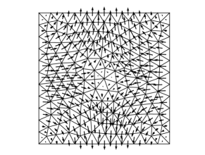
Figure 9: The first 50 nonzero eigenvalues for the resonant cavity problem of Section 11.1 and the eigenvector corresponding to one of these eigenvalues. The eigenvector is a 1-cochain which is visualized as a vector field by first interpolating it using a Whitney map. See Section 11.1 for details.

11.2 Darcy flow or Poisson’s in mixed form

We give here a brief description of the equations of Darcy flow and their PyDEC implementation. For more details see [34]. The resonant cavity example in Section 11.1 was implemented using finite element exterior calculus. For variety we use a DEC implementation for Darcy flow.

Darcy flow is a simple model of steady state flow of an incompressible fluid in a porous medium. It models the statement that flow is from high to low pressure. For a fixed pressure gradient, the velocity is proportional to the permeability $\kappa$ of the medium and inversely proportional to the viscosity $\mu$ of the fluid. Let the domain be $M$, a polygonal planar domain. Assuming that there are no sources of fluid in $M$ and there is no other force acting on the fluid, the equations of Darcy flow are

$$v+\frac{\kappa}{\mu}\nabla p=0\quad\text{and}\quad\operatorname{div}v=0\quad\text{in }M\quad\text{with}\quad v\cdot\hat{n}=\psi\quad\text{on }\partial M.$$ (11.1)

where $\kappa>0$ is the coefficient of permeability of the medium $\mu>0$ is the coefficient of (dynamic) viscosity of the fluid, $\psi:\partial M\rightarrow\mathbb{R}$ is the prescribed normal component of the velocity across the boundary, and $\hat{n}$ is the unit outward normal vector to $\partial M$. For consistency $\int_{\partial M}\psi\,d\Gamma=0$, where $d\Gamma$ is the measure on $\partial M$. Since $\operatorname{div}\circ\operatorname{grad}=\Delta$, the simplified Darcy flow equations above are equivalent to Laplace’s equation.

Let $K$ be a simplicial complex that triangulates $M$. Instead of velocity and pressure, we will use flux and pressure as the primary unknowns. The flux through the edges is $f=\operatorname{\ast}v^{\flat}$ and thus it will be a primal 1-cochain. Although PyDEC does not implement a flat operator, this is not an issue here because we never solve for $v$, and make $f$ itself one of the unknowns. This implies that the pressure $p$ will be a dual 0-cochain since $\operatorname{\ast}\operatorname{d}p$ has to be of the same type as $f$. The choice to put flux on primal edges and pressures on circumcenters can be reversed, as shown in a dual formulation in [26]. In exterior calculus notation, the PDE in (11.1) is $-(\mu/k)\operatorname{\ast}f+\operatorname{d}p=0$ and $\operatorname{d}f=0$, which, when discretized, translates to the matrix equation

$$\begin{bmatrix}-(\mu/k)\operatorname{\ast}_{1}&\operatorname{d}_{1}^{T}\\ \operatorname{d}_{1}&0\end{bmatrix}\begin{bmatrix}f\\ p\end{bmatrix}=\begin{bmatrix}0\\ 0\end{bmatrix}\,.$$

In PyDEC, the construction of this matrix is straightforward. Once a simplicial complex sc has been constructed, the following 3 lines construct the matrix in the system above :

⬇

d1 = sc[1].d; star1 = sc[1].star

A = bmat([[(-mu/k)*sc[1].star, sc[1].d.T],

[sc[1].d, None]], format=’csr’)

After computing the boundary condition in terms of flux through the boundary edges, the linear system is adjusted for the known values and then solved for the fluxes and pressures. Figure 10 shows the solution for the case of constant horizontal velocity and linear pressure gradient.

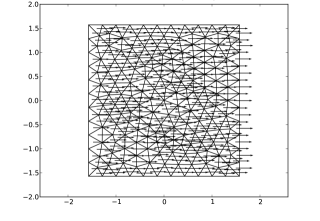
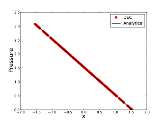
Figure 10: Darcy flow using discrete exterior calculus. The boundary condition is that fluid is coming in from left and leaving from right with velocity 1. The velocity inside should be constant and pressure should be linear. The flux and pressure are computed in a mixed formulation. The flux is taken to be a primal 1-cochain associated with primal edges, and the pressure is a dual 0-cochain on dual vertices, which are circumcenters of the triangles. The velocity is obtained by Whitney interpolation of the flux, which is sampled at the barycenters. See Section 11.2 for more details.

11.3 Cohomology basis using Hodge decomposition

The Hodge Decomposition Theorem [1, page 539] states that for a compact boundaryless smooth manifold $M$, for any $p$-form $\omega\in\Omega^{p}(M)$, there exists an $\alpha\in\Omega^{p-1}(M)$, $\beta\in\Omega^{p+1}(M)$, and a harmonic form $h\in\Omega^{p}(M)$ such that $\omega=d\alpha+\delta\beta+h$. Here harmonic means that $\Delta h=0$, where $\Delta$ is the Laplace-deRham operator $\operatorname{d}\delta+\delta\operatorname{d}$. Moreover $\operatorname{d}\alpha$, $\delta\beta$ and $h$ are mutually $L^{2}$-orthogonal, which makes them uniquely determined. In case of a manifold with boundary, the decomposition is similar, with some additional boundary conditions. See [1] for details.

The Hodge-deRham theorem [1], relates the analytical concept of harmonic forms with the topological concept of cohomology. For any topological space, the cohomology groups or vector spaces of various dimension capture essential topological information about the space [45]. For the manifold $M$ above, the $p$-dimensional cohomology group with real coefficients, which is a finite-dimensional space, is denoted $H^{p}(M;\mathbb{R})$ or just $H^{p}(M)$. For example, for a torus, $H^{1}$ has dimension 2. For a square with 4 holes used in this example, which does have boundaries, $H^{1}$ has dimension 4. The elements of $H^{p}(M)$ are equivalence classes of closed forms (those whose $\operatorname{d}$ is 0). Two closed forms are equivalent if their difference is exact (that is, is $\operatorname{d}$ of some form). While the representatives of 1-homology spaces can be visualized as loops around holes, handles, and tunnels, those of 1-cohomology should be visualized as fields. If the space of harmonic forms is denoted $\mathcal{H}^{p}(M)$, then the Hodge-deRham theorem says that it is isomorphic, as a vector space, to the $p$-th cohomology space $H^{p}(M)$ in the case of a closed manifold. See [38] for details. Again, the case of $M$ with boundary requires some adjustments in the definitions, as given in [1].

For finite dimensional spaces, Hodge decomposition follows from very elementary linear algebra. If $U$, $V$ and $W$ are finite-dimensional inner product vector spaces and $A:U\to V$ and $B:V\to W$ are linear maps such that $B\circ A=0$ then middle vector space $V$ splits into 3 orthogonal components, which are $\operatorname{im}A$, $\operatorname{im}B^{T}$, and $\ker A^{T}\cap\ker B$. In this example, we find a basis for $H^{1}$ for a square. This is done by finding a basis of harmonic 1-cochains. Thus given a 1-cochain $\omega$, its discrete Hodge decomposition exists and is $\omega=\operatorname{d}_{0}\alpha+\operatorname{\delta}_{2}\beta+h$. In this example, the cochains $\alpha$ and $\beta$ are obtained by solving the linear systems $\operatorname{\delta}_{1}\operatorname{d}_{0}\alpha=\operatorname{\delta}_{1}\omega$ and $\operatorname{d}_{1}\operatorname{\delta}_{2}\beta=\operatorname{d}_{1}\omega$. The harmonic component can then be computed by subtraction.

In the example code, the main function is the one that computes the Hodge decomposition of a given cochain omega. First empty cochains for alpha and beta are created:

⬇

sc = omega.complex

p = omega.k

alpha = sc.get_cochain(p - 1)

beta = sc.get_cochain(p + 1)

Now the solution for alpha and beta closely follows the above equations for $\alpha$ and $\beta$:

⬇

A = delta(d(sc.get_cochain_basis(p - 1))).v

b = delta(omega).v

alpha.v = cg( A, b, tol=1e-8 )[0]

⬇

A = d(delta(sc.get_cochain_basis(p + 1))).v

b = d(omega).v

beta.v = cg( A, b, tol=1e-8 )[0]

Even though the matrices A above are singular, the solutions exist, and since conjugate gradient is used, the presence of the nontrivial kernels does not pose any problems [9].

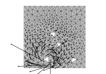
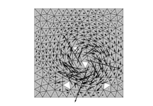
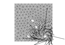
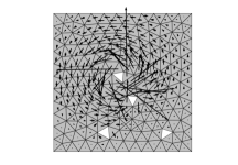
Figure 11: Four harmonic cochains form a basis for the first cohomology space $H^{1}$ for a mesh with four holes. Each cochain is visualized above as a vector field by interpolating it from the edge values using Whitney interpolation. See Section 11.3 for details.

The harmonic $1$-forms shown in Figure 11 are obtained by decomposing random $1$-forms and retaining their harmonic components. Since the initial basis has no particular spatial structure, an ad hoc orthogonalization procedure is then applied. For each basis vector, the algorithm identifies the component with the maximum magnitude and applies Householder transforms to force the other vectors to zero at that same component.

11.4 Sensor network coverage

As discussed in Section 5, sensor network coverage gaps can be identified with coordinate-free methods based on topological properties of the Rips complex. This is for an idealized abstraction of a sensor network. The following example constructs a rips_complex object from a set of 300 points randomly distributed over the unit square, as illustrated in top left in Figure 12. Recall that the Rips complex is constructed by adding an edge between each pair each pair of points within a given radius. Top right of Figure 12 illustrates the edges of the Rips complex produced by a cut-off radius of 0.15. The triangles of the Rips complex, illustrated in bottom left of Figure 12, represent triplets of vertices that form a clique in the edge graph of the Rips complex. The Rips complex is created by the following two lines of code

⬇

pts = read_array(’300pts.mtx’) # 300 random points in 2D

rc = rips_complex( pts, 0.15 )

The sensor network is tested for coverage holes by inspecting the kernel of the matrix $\Delta_{1}=\operatorname{\partial}_{1}^{T}\operatorname{\partial}_{1}+\operatorname{\partial}_{2}\operatorname{\partial}_{2}^{T}$ [17]. Specifically, null-vectors of $\Delta_{1}$, which are called harmonic 1-cochains (by analogy with the definition of harmonic cochains used in the previous subsection), reveal the presence of holes in the sensor network. In this example we explore the kernel of $\Delta_{1}$ by generating a random 1-cochain x and extracting its harmonic part using a discrete hodge decomposition as outlined in the previous subsection. If the harmonic component of x is (numerically) zero then we may conclude with high confidence that $\Delta_{1}$ is nonsingular and that no holes are present. However, in this case the hodge decomposition of x produces a nonzero harmonic component h. Indeed, plotting h on the edges of the Rips complex localizes the coverage hole, as the bottom right of Figure 12 demonstrates.

To set up the linear systems, the boundary matrices are obtained from the Rips complex rc created above:

⬇

cmplx = rc.chain_complex() # boundary operators [ b0, b1, b2 ]

b1 = cmplx[1].astype(float) # edge boundary operator

b2 = cmplx[2].astype(float) # face boundary operator

Then the random cochain is created and the Hodge decomposition computed, to find the harmonic cochain which is then normalized:

⬇

x = rand(b1.shape[1]) # random 1-chain

# Decompose x using discrete Hodge decomposition

alpha = cg( b1 * b1.T, b1 * x, tol=1e-8)[0]

beta = cg( b2.T * b2, b2.T * x, tol=1e-8)[0]

h = x - (b1.T * alpha) - (b2 * beta) # harmonic component of x

h /= abs(h).max() # normalize h

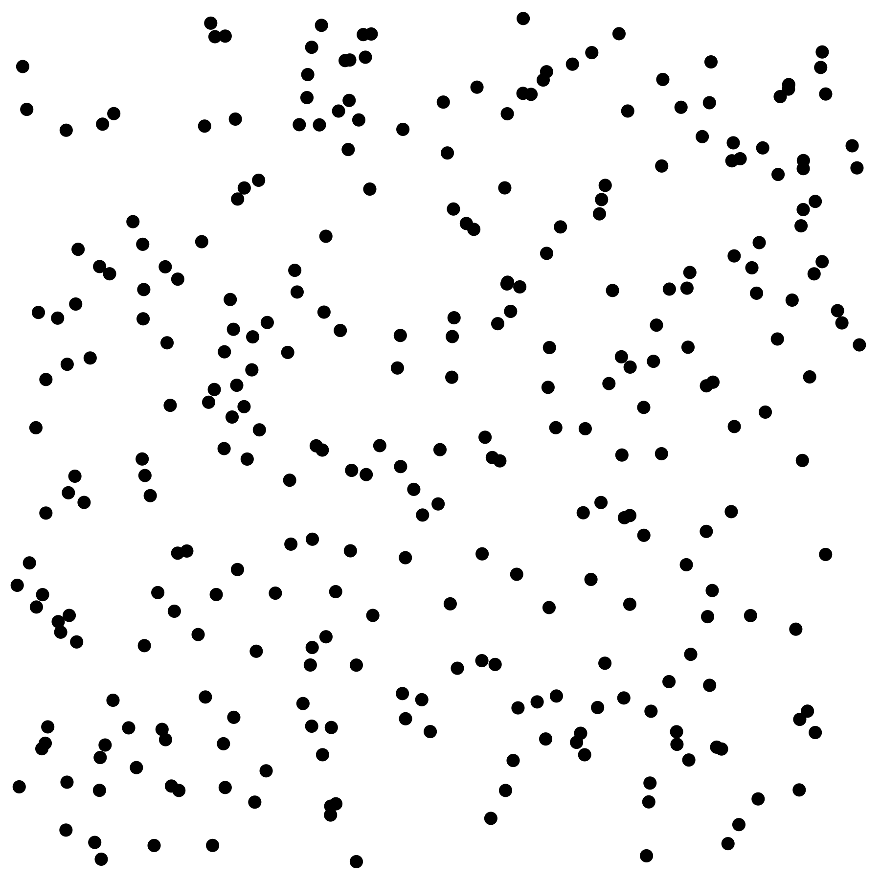
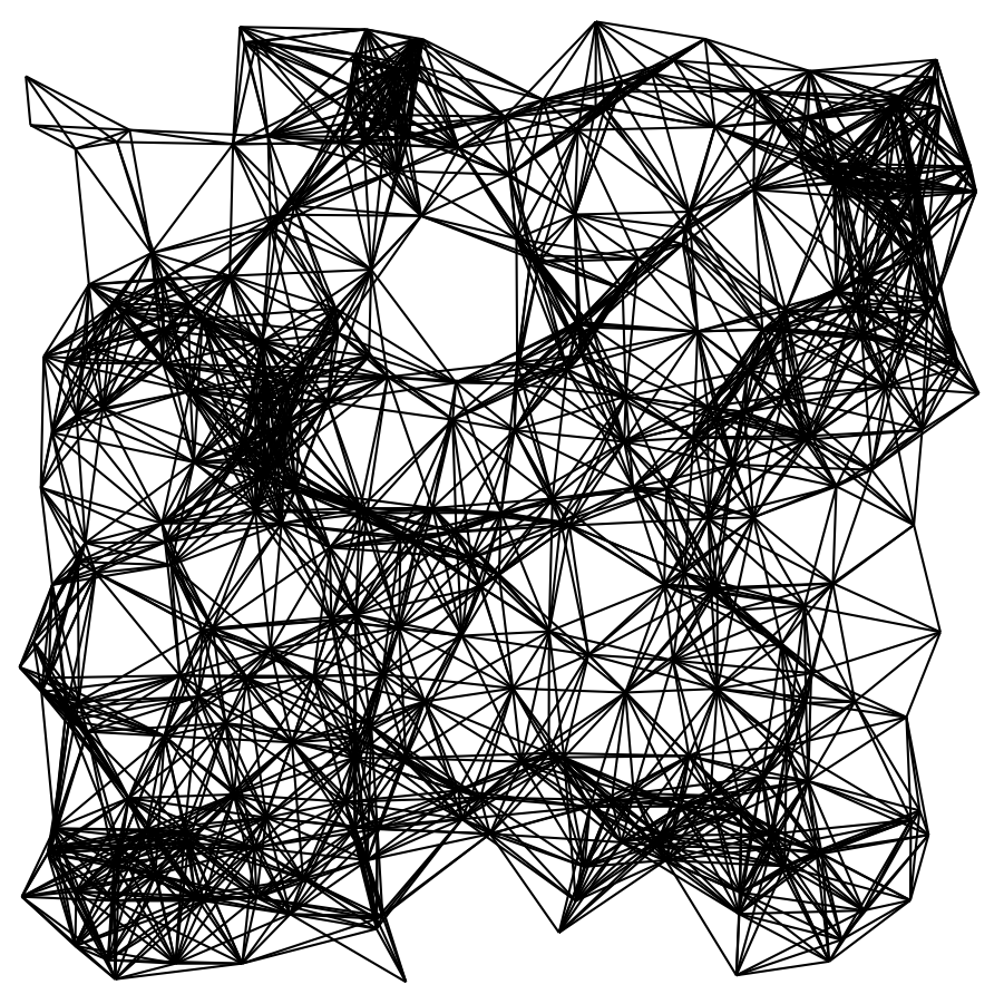
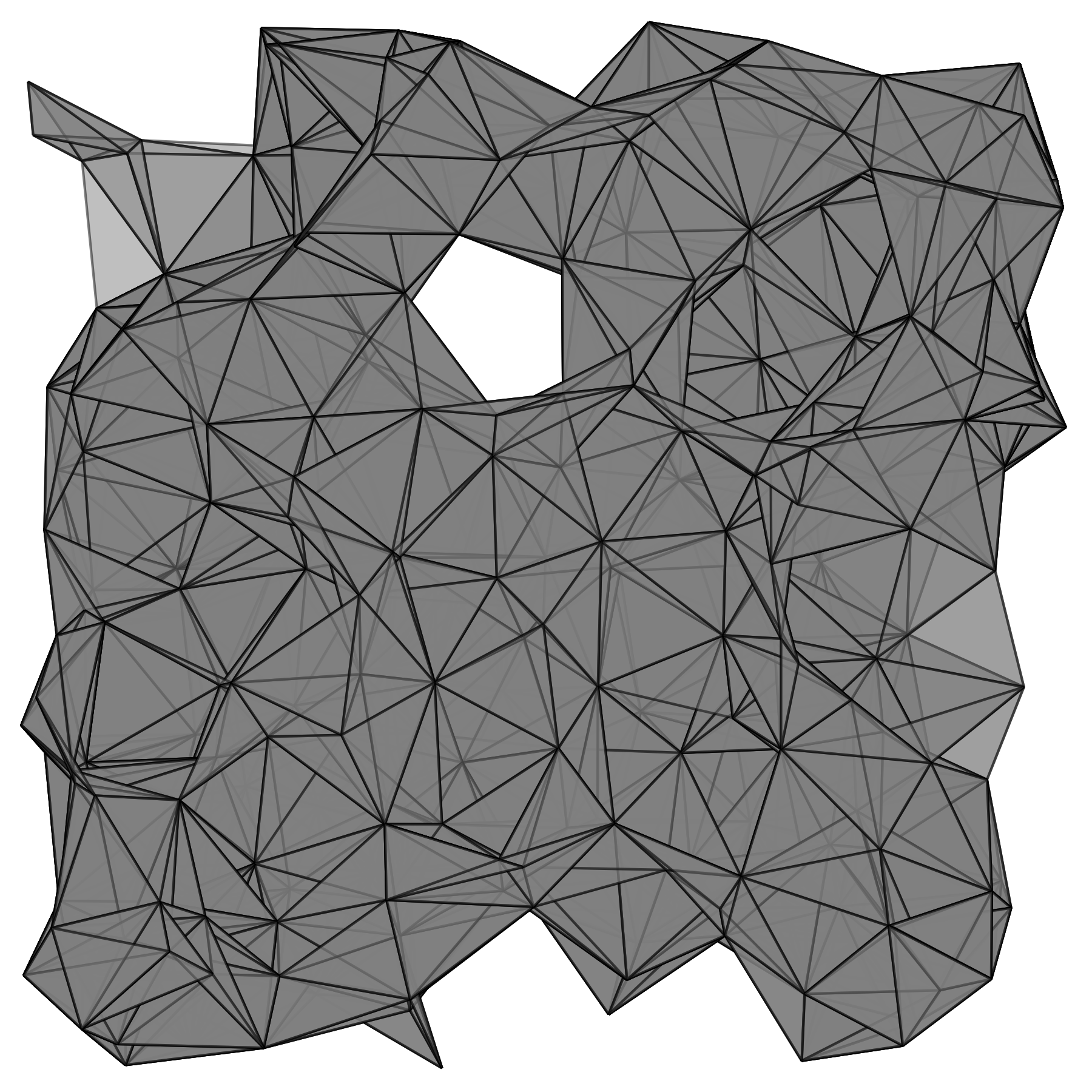
Figure 12: Hodge decomposition for finding coverage holes in an idealized sensor network. Top left shows a sample sensor network with 300 randomly distributed points. Pairs of points within a fixed distance of one another are connected by an edge and this is shown on top right. Triangles are added to the Rips complex when three points form a clique (complete graph). These are shown in bottom left. The existence of a harmonic 1-cochain indicates a potential hole in the sensor network coverage. In the bottom right figure, edge thickness reflects the magnitude of the harmonic cochain on each edge. See Section 11.4 for more details.

11.5 Least squares ranking on graphs

This is a formulation for ranking alternatives based on pairwise data. Given is a collection of alternatives or objects that have to be ranked, by computing a ranking score that sorts them. The ranking scores are to be computed starting from some pairwise comparisons. Some examples of objects to be ranked are basketball teams, movies, candidates for a job. Typically, the given data will not have pairwise comparisons for all the possible pairs. There is no geometry in this application, hence no exterior calculus is involved. PyDEC however still proves useful because the full version of this example [33] uses an abstract simplicial 2-complex. Thus PyDEC is useful in forming the complex and for determining its boundary matrix. In this simplified example, only an abstract simplicial 1-complex is needed.

Form a simple graph $G$, with the objects to be ranked being the vertices and with an edge between any two which have pairwise comparison data given. If there are $n$ objects, possibly only a sparse subset out of all possible $O(n^{2})$ pairs may have comparison data associated with them. Here we’ll only require that the graph be connected. This condition can be dropped with the consequence that the rankings of separate components become independent of each other. The comparison values are real numbers.

Since $G$ is a simple graph, by orienting the edges arbitrarily it becomes an oriented 1-dimensional abstract simplicial complex. The vector $\omega$ of pairwise comparison values is a 1-cochain since if A is preferred over B by, say, $4$ points, then B is preferred over A by $-4$ points.

The ranking scores $\alpha$ which are to be computed on vertices form a 0-cochain. For any edge $e=(u,v)$ from vertex $u$ to vertex $v$, the difference of vertex values $\alpha(v)-\alpha(u)$ should match $\omega(e)$ as much as possible, for example, in a least squares sense. This idea is from [40] who proposed it as a method for ranking football teams. By including the 3-cliques as triangles, $G$ becomes a 2-dimensional simplicial complex. This was used in [37] to extend this ranking idea. In [37] the computation of the scores $\alpha$ is interpreted as one part of the Hodge decomposition of $\omega$. See Section 11.3 above for a basic discussion of Hodge decomposition where it is used for computing harmonic cochains on a mesh. Here we will just compute the ranking score $\alpha$. This is done by solving the least squares problem $\operatorname{\partial}_{1}^{T}\,\alpha\simeq\omega$.

The graph in this example is used for ranking basketball teams, using real data for a small subset of American Men’s college basketball games from 2010-2011 season. Each team is a node in the graph and has been given a number as a name. An edge between two teams indicates that one of more games have been played between them. The score difference from these games becomes the input 1-cochain $\omega$, with one value on each edge. If multiple games were played by a pair the score differences were added to create this data. The data is stored as a matrix in which the first two columns are the teams and the third column is the value of the 1-cochain on that edge.

Once this data is loaded from file, an abstract simplicial complex is created from the first two columns which form the edges of the graph. The loading and complex creation is done by the following few lines of code

⬇

data = loadtxt(’data.txt’).astype(int)

edges = data[:,:2]

# Create abstract simplicial complex from edges

asc = abstract_simplicial_complex([edges])

In PyDEC, the simplices that are given as input to construct a complex are preserved as is. Lower dimensional simplices that are derived from them are stored and oriented in sorted order. Thus in the above data, the edge between node 8 and 1 will be oriented from 8 to 1. The above example data may mean, for example, that team labelled 1 lost to team labelled 8 by 9 points.

The 1-cochain $\omega$ is now extracted from the data array and the boundary matrix needed is obtained from the complex and the least squares problem solved. All this is accomplished in the following lines

⬇

omega = data[:,-1] # pairwise comparisons

B1 = asc.chain_complex()[1] # boundary matrix

alpha = lsqr(B1.T, omega)[0] # solve least squares problem

The resulting alpha values computed are given below.

$$\begin{array}[]{lccccccccccc}\text{Team number}&0&1&2&3&4&5&6&7&8&9&10\\ \alpha\text{ value}&14.5&2.0&0.0&7.2&5.9&9.0&2.3&23.6&11.0&23.8&21.7\end{array}$$

The team with $\alpha=0$ is the worst team according to these rankings and the one with the largest $\alpha$ value (23.8 here) is the best team. Note that the score difference from the game between 8 and 1 happens to be exactly the difference in $\alpha$ values between them. This won’t always be true. See for example teams 3 and 9. Such discrepancies come from having a residual in the least squares solution, and that is a direct result of the presence of cycles in the graph. In fact it may even happen that team A beats B, which beats C, which in turn beats A. Thus no assignment of $\alpha$ values will resolve this inconsistency. This is where a second least squares problem and hence a Hodge decomposition plays a role. The second problem is not considered in this example. See [33] for details on the second least squares problem and the role of Hodge decomposition and harmonic cochains in the ranking context.

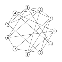
Figure 13: A typical graph of a subset of basketball games. Each node is a team, labelled by a number. An edge represents one or more games played by the two teams connected by it. The actual graph used in the example in Section 11.5 is a complete graph.

12 Conclusions

PyDEC is intended to be a tool for solving elliptic PDEs formulated in terms of differential forms and for exploring computational topology problems. It has been used for numerical experiments for Darcy flow [34], computation of harmonic cochains on two and three dimensional meshes [32], and least squares ranking on graphs [33]. It has also proved valuable in computational topology work [20, 22], for creating complexes and computing boundary matrices. The design goals for PyDEC have been efficiency and ability to express mathematical formulations easily. Section 11 which described some examples should give an idea of how close the PyDEC code is to the mathematical formulation of the problems considered. Many packages exist and are being created for numerical PDE solutions using differential forms. There are also many excellent computational topology packages. PyDEC can handle a large variety of complexes and provides implementations of discrete exterior calculus and lowest order finite element exterior calculus using Whitney forms. These qualities make it a convenient tool to explore the interrelationships between topology, geometry, and numerical PDEs.

Appendix

Proof of Proposition 9.7: By definition $M_{p}(i,j)=\int_{\lvert K\rvert}\bigl{\langle}\operatorname{W}\bigl{(}\sigma^{p}_{i}\bigr{)}^{\ast},\operatorname{W}\bigl{(}\sigma^{p}_{j}\bigr{)}^{\ast}\bigr{\rangle}\mu$. The integrand is nonzero only in $\operatorname{\overline{St}}(\sigma^{p}_{i})\cap\operatorname{\overline{St}}(\sigma^{p}_{i})$ since the Whitney form corresponding to a simplex is zero outside the star of that simplex [21]. Thus

$$M_{p}(i,j)=\underset{\sigma^{n}\succeq\sigma^{p}_{i},\sigma^{p}_{j}}{\sum_{\sigma_{n}}}\int_{\sigma_{n}}\bigl{\langle}\operatorname{W}\bigl{(}\sigma^{p}_{i}\bigr{)}^{\ast}\bigr{|}_{\sigma^{n}},\operatorname{W}\bigl{(}\sigma^{p}_{j}\bigr{)}^{\ast}\bigr{|}_{\sigma^{n}}\bigr{\rangle}\mu\,.$$

By the definition of the Whitney map, $M_{p}(i,j)$ is

$$(p!)^{2}\underset{\sigma^{n}\succeq\sigma^{p}_{i},\sigma^{p}_{j}}{\sum_{\sigma^{n}}}\sum_{k,l=0}^{p}(-1)^{k+l}\\ \int_{\sigma^{n}}\bigl{\langle}\operatorname{d}\mu_{i_{0}}\wedge\dots\widehat{\operatorname{d}\mu_{i_{k}}}\dots\wedge\operatorname{d}\mu_{i_{p}},\operatorname{d}\mu_{j_{0}}\wedge\dots\widehat{\operatorname{d}\mu_{j_{l}}}\dots\wedge\operatorname{d}\mu_{j_{p}}\bigr{\rangle}\mu_{i_{k}}\mu_{j_{l}}\,\mu\,.$$

But differentials of barycentric coordinates are constant in $\sigma^{n}$. Thus the term

$$\bigl{\langle}\operatorname{d}\mu_{i_{0}}\wedge\dots\widehat{\operatorname{d}\mu_{i_{k}}}\dots\wedge\operatorname{d}\mu_{i_{p}},\operatorname{d}\mu_{j_{0}}\wedge\dots\widehat{\operatorname{d}\mu_{j_{l}}}\dots\wedge\operatorname{d}\mu_{j_{p}}\bigr{\rangle}$$

comes out of the integral. Recalling Definition 8.2 of inner product of forms,

$$\bigl{\langle}\operatorname{d}\mu_{i_{0}}\wedge\dots\widehat{\operatorname{d}\mu_{i_{k}}}\dots\wedge\operatorname{d}\mu_{i_{p}},\operatorname{d}\mu_{j_{0}}\wedge\dots\widehat{\operatorname{d}\mu_{j_{l}}}\dots\wedge\operatorname{d}\mu_{j_{p}}\bigr{\rangle}$$

is given by

$$\det\begin{bmatrix}\bigl{\langle}\operatorname{d}\mu_{i_{0}},\operatorname{d}\mu_{j_{0}}\bigr{\rangle}&\dots&\widehat{\bigl{\langle}\operatorname{d}\mu_{i_{0}},\operatorname{d}\mu_{j_{l}}\bigr{\rangle}}&\dots&\bigl{\langle}\operatorname{d}\mu_{i_{0}},\operatorname{d}\mu_{j_{p}}\bigr{\rangle}\\ \vdots&&\vdots&&\vdots\\ \widehat{\bigl{\langle}\operatorname{d}\mu_{i_{k}},\operatorname{d}\mu_{j_{0}}\bigr{\rangle}}&\dots&\widehat{\bigl{\langle}\operatorname{d}\mu_{i_{k}},\operatorname{d}\mu_{j_{l}}\bigr{\rangle}}&\dots&\widehat{\bigl{\langle}\operatorname{d}\mu_{i_{k}},\operatorname{d}\mu_{j_{l}}\bigr{\rangle}}\\ \vdots&&\vdots&&\vdots\\ \bigl{\langle}\operatorname{d}\mu_{i_{p}},\operatorname{d}\mu_{j_{0}}\bigr{\rangle}&\dots&\widehat{\bigl{\langle}\operatorname{d}\mu_{i_{p}},\operatorname{d}\mu_{j_{l}}\bigr{\rangle}}&\dots&\bigl{\langle}\operatorname{d}\mu_{i_{p}},\operatorname{d}\mu_{j_{p}}\bigr{\rangle}\end{bmatrix}\,,$$

which completes the proof.

References

- [1] Abraham, R., Marsden, J. E., and Ratiu, T. Manifolds, Tensor Analysis, and Applications, second ed. Springer–Verlag, New York, 1988.
- [2] Arnold, D. N., Falk, R. S., and Winther, R. Finite element exterior calculus, homological techniques, and applications. In Acta Numerica, A. Iserles, Ed., vol. 15. Cambridge University Press, 2006, pp. 1–155.
- [3] Arnold, D. N., Falk, R. S., and Winther, R. Geometric decompositions and local bases for spaces of finite element differential forms. Comput. Methods Appl. Mech. Engrg. 198, 21-26 (2009), 1660–1672. doi:10.1016/j.cma.2008.12.017.
- [4] Arnold, D. N., Falk, R. S., and Winther, R. Finite element exterior calculus: from Hodge theory to numerical stability. Bull. Amer. Math. Soc. (N.S.) 47, 2 (2010), 281–354. doi:10.1090/S0273-0979-10-01278-4.
- [5] Bangerth, W., Hartmann, R., and Kanschat, G. deal.II – a general purpose object oriented finite element library. ACM Trans. Math. Softw. 33, 4 (2007), 24/1–24/27.
- [6] Bank, R., and Douglas, C. Sparse matrix multiplication package (SMMP). Advances in Computational Mathematics 1, 1 (1993), 127–137.
- [7] Bell, N., and Hirani, A. N. PyDEC: A Python library for Discrete Exterior Calculus [online]. Software made available on Google Code website.
- [8] Bell, W. N. Algebraic Multigrid for Discrete Differential Forms. PhD thesis, University of Illinois at Urbana-Champaign, Urbana, Illinois, 2008.
- [9] Bochev, P., and Lehoucq, R. B. On the finite element solution of the pure Neumann problem. SIAM Review 47, 1 (2005), 50–66. doi:10.1137/S0036144503426074.
- [10] Bochev, P. B., and Hyman, J. M. Principles of mimetic discretizations of differential operators. In Compatible Spatial Discretizations, D. N. Arnold, P. B. Bochev, R. B. Lehoucq, R. A. Nicolaides, and M. Shashkov, Eds., vol. 142 of The IMA Volumes in Mathematics and its Applications. Springer, Berlin, 2006, pp. 89–119.
- [11] Bochev, P. B., and Robinson, A. C. Matching algorithms with physics: exact sequences of finite element spaces. In Collected Lectures on Preservation of Stability Under Discretization, D. Estep and S. Tavener, Eds. Society for Industrial and Applied Mathematics (SIAM), 2002, ch. 8, pp. 145–166.
- [12] Boffi, D., Fernandes, P., Gastaldi, L., and Perugia, I. Computational models of electromagnetic resonators: analysis of edge element approximation. SIAM J. Numer. Anal. 36, 4 (1999), 1264–1290 (electronic).
- [13] Bossavit, A. Whitney forms : A class of finite elements for three-dimensional computations in electromagnetism. IEE Proceedings 135, Part A, 8 (November 1988), 493–500.
- [14] Bott, R., and Tu, L. W. Differential Forms in Algebraic Topology. Springer–Verlag, New York, 1982.
- [15] Castillo, P., Rieben, R., and White, D. FEMSTER: An object oriented class library of high-order discrete differential forms. ACM Transactions on Mathematical Software 31, 4 (Dec. 2005), 425–457.
- [16] de Rham, G. Variétés différentiables. Formes, courants, formes harmoniques. Actualités Sci. Ind., no. 1222 = Publ. Inst. Math. Univ. Nancago III. Hermann et Cie, Paris, 1955.
- [17] de Silva, V., and Ghrist, R. Homological sensor networks. Notices of the American Mathematical Society 54, 1 (2007), 10–17.
- [18] Demlow, A., and Dziuk, G. An adaptive finite element method for the Laplace–Beltrami operator on implicitly defined surfaces. SIAM Journal on Numerical Analysis 45, 1 (2007), 421–442. doi:10.1137/050642873.
- [19] Desbrun, M., Hirani, A. N., Leok, M., and Marsden, J. E. Discrete exterior calculus, August 2005. arXiv:math.DG/0508341.
- [20] Dey, T. K., Hirani, A. N., and Krishnamoorthy, B. Optimal homologous cycles, total unimodularity, and linear programming. In STOC ’10: Proceedings of the 42nd ACM Symposium on Theory of Computing (New York, NY, USA, June 6–8 2010), ACM, pp. 221–230. doi:10.1145/1806689.1806721.
- [21] Dodziuk, J. Finite-difference approach to the Hodge theory of harmonic forms. Amer. J. Math. 98, 1 (1976), 79–104.
- [22] Dunfield, N. M., and Hirani, A. N. The least spanning area of a knot and the optimal bounding chain problem. In Proceedings of the 27th annual ACM symposium on Computational geometry (New York, NY, USA, 2011), SoCG ’11, ACM, pp. 135–144. doi:%****␣pydec.bbl␣Line␣150␣****10.1145/1998196.1998218.
- [23] Eckmann, B. Harmonische Funktionen und Randwertaufgaben in einem Komplex. Comment. Math. Helv. 17 (1945), 240–255. doi:10.1007/BF02566245.
- [24] Edelsbrunner, H., Letscher, D., and Zomorodian, A. Topological persistence and simplification. Discrete and Computational Geometry 28, 4 (November 2002), 511–533. doi:10.1007/s00454-002-2885-2.
- [25] Frankel, T. The Geometry of Physics, second ed. Cambridge University Press, Cambridge, 2004. An introduction.
- [26] Gillette, A., and Bajaj, C. Dual formulations of mixed finite element methods, 2010. arXiv:1012.3929v3.
- [27] Gillette, A., and Bajaj, C. A generalization for stable mixed finite elements. In SPM ’10: Proceedings of the 14th ACM Symposium on Solid and Physical Modeling (New York, NY, USA, 2010), ACM, pp. 41–50. doi:10.1145/1839778.1839785.
- [28] Gradinaru, V., and Hiptmair, R. Whitney elements on pyramids. Electronic Transactions on Numerical Analysis 8 (1999), 154–168.
- [29] Hildebrandt, K., Polthier, K., and Wardetzky, M. On the convergence of metric and geometric properties of polyhedral surfaces. Geom. Dedicata 123 (2006), 89–112. doi:10.1007/s10711-006-9109-5.
- [30] Hiptmair, R. Finite elements in computational electromagnetism. In Acta Numerica, A. Iserles, Ed., vol. 11. Cambridge University Press, 2002, pp. 237–339.
- [31] Hirani, A. N. Discrete Exterior Calculus. PhD thesis, California Institute of Technology, May 2003.
- [32] Hirani, A. N., Kalyanaraman, K., Wang, H., and Watts, S. Cohomologous harmonic cochains, 2011. arXiv:1012.2835.
- [33] Hirani, A. N., Kalyanaraman, K., and Watts, S. Least squares ranking on graphs, 2011. arXiv:1011.1716.
- [34] Hirani, A. N., Nakshatrala, K. B., and Chaudhry, J. H. Numerical method for Darcy flow derived using Discrete Exterior Calculus, 2011. arXiv:0810.3434.
- [35] Holst, M., and Stern, A. Geometric variational crimes: Hilbert complexes, finite element exterior calculus, and problems on hypersurfaces, May 2011. arXiv:1005.4455.
- [36] Hyman, J. M., and Shashkov, M. Natural discretizations for the divergence, gradient, and curl on logically rectangular grids. Comput. Math. Appl. 33, 4 (1997), 81–104. doi:10.1016/S0898-1221(97)00009-6.
- [37] Jiang, X., Lim, L.-H., Yao, Y., and Ye, Y. Statistical ranking and combinatorial hodge theory. Mathematical Programming 127 (2011), 203–244. doi:10.1007/s10107-010-0419-x.
- [38] Jost, J. Riemannian Geometry and Geometric Analysis, fourth ed. Universitext. Springer-Verlag, Berlin, 2005. doi:10.1007/3-540-28890-2.
- [39] Kaczynski, T., Mischaikow, K., and Mrozek, M. Computational homology, vol. 157 of Applied Mathematical Sciences. Springer-Verlag, New York, 2004.
- [40] Leake, R. J. A method for ranking teams: With an application to college football. In Management Science in Sports, R. E. Machol and S. P. Ladany, Eds., vol. 4 of TIMS Studies in the Management Sciences. North-Holland Publishing Company, 1976, pp. 27–46.
- [41] Logg, A., and Mardal, K.-A. A symbolic engine for finite element exterior calculus. Talk at European Finite Element Fair, May 2008.
- [42] Logg, A., Mardal, K.-A., Wells, G. N., et al. Automated Solution of Differential Equations by the Finite Element Method. Springer, 2012.
- [43] Logg, A., and Wells, G. N. DOLFIN: Automated finite element computing. ACM Trans. Math. Softw. 37 (April 2010), 20:1–20:28. doi:http://doi.acm.org/10.1145/1731022.1731030.
- [44] Morita, S. Geometry of Differential Forms, vol. 201 of Translations of Mathematical Monographs. American Mathematical Society, Providence, RI, 2001.
- [45] Munkres, J. R. Elements of Algebraic Topology. Addison–Wesley Publishing Company, Menlo Park, 1984.
- [46] Nicolaides, R. A., and Trapp, K. A. Covolume discretization of differential forms. In Compatible Spatial Discretizations, D. N. Arnold, P. B. Bochev, R. B. Lehoucq, R. A. Nicolaides, and M. Shashkov, Eds., vol. 142 of The IMA Volumes in Mathematics and its Applications. Springer, New York, 2006, pp. 161–171.
- [47] Oliphant, T. E. Python for scientific computing. Computing in Science & Engineering 9, 3 (2007), 10–20.
- [48] Saad, Y. Iterative Methods for Sparse Linear Systems, second ed. Society for Industrial and Applied Mathematics, Philadelphia, PA, 2003.
- [49] Sen, S. A cubic Whitney and further developments in geometric discretisation. arXiv:hep-th/0307166v2 (2003), Online.
- [50] Shashkov, M. Conservative finite-difference methods on general grids. CRC Press, Boca Raton, FL, 1996.
- [51] van der Walt, S., Colbert, S., and Varoquaux, G. The NumPy array: A structure for efficient numerical computation. Computing in Science Engineering 13, 2 (2011), 22–30. doi:10.1109/MCSE.2011.37.
- [52] Whitney, H. Geometric Integration Theory. Princeton University Press, Princeton, N. J., 1957.
- [53] Wilson, S. Cochain algebra on manifolds and convergence under refinement. Topology and its Applications 154, 9 (May 2007), 1898–1920. doi:10.1016/j.topol.2007.01.017.
- [54] Wilson, S. O. Conformal cochains. Transactions of the American Mathematical Society 360 (2008), 5247–5264.
- [55] Zomorodian, A., and Carlsson, G. Computing persistent homology. Discrete and Computational Geometry 33, 2 (February 2005), 249–274. doi:10.1007/s00454-004-1146-y.