Connectivity Damage to a Graph
by the Removal of an Edge or a Vertex

Abstract

The approach of quantifying the damage inflicted on a graph in Albert, Jeong and Barabási’s (AJB) report “Error and Attack Tolerance of Complex Networks” using the size of the largest connected component and the average size of the remaining components does not capture our intuitive idea of the damage to a graph caused by disconnections. We evaluate an alternative metric based on average inverse path lengths (AIPLs) that better fits our intuition that a graph can still be reasonably functional even when it is disconnected. We compare our metric with AJB’s using a test set of graphs and report the differences. AJB’s report should not be confused with a report by Crucitti et al. with the same name.

Based on our analysis of graphs of different sizes and types, and using various numerical and statistical tools; the ratio of the average inverse path lengths of a connected graph of the same size as the sum of the size of the fragments of the disconnected graph can be used as a metric about the damage of a graph by the removal of an edge or a node. This damage is reported in the range (0,1) where 0 means that the removal had no effect on the graph’s capability to perform its functions. A 1 means that the graph is totally dysfunctional. We exercise our metric on a collection of sample graphs that have been subjected to various attack profiles that focus on edge, node or degree betweenness values.

We believe that this metric can be used to quantify the damage done to the graph by an attacker, and that it can be used in evaluating the positive effect of adding additional edges to an existing graph.

1 Introduction

The likelihood of a graph, or network to remain functional in the face of random failures and directed attacks has been the interest to many different authors. In attempting to understand the problem and their root causes; we reviewed [2, 11, 13, 12, 14, 23, 10, 20, 4, 27, 19, 21, 18, 8]. Our desire is to have a single value that could be used across graphs as an indicator of the graph’s “damage,” “robustness,” or “general health.” This value would be applicable whether or not the graph was connected or disconnected.

The paper documents the approach used to arrive at a single metric that can be used to report the damage caused to the graph by the removal of either an edge or a vertex. The complement of this damage estimate would be the “health” of a graph by the addition of an edge. Included are the supporting equations, the data used to test main stream and “corner” test cases and an analysis of the results.

Our sense is that a graph may still perform most of its duties (i.e., communicate between nodes, maintain data in a node, respond to queries, etc.) even when it may not be able to perform those functions between any arbitrary nodes $u$ and $v$. In this sense, a graph may be connected or disconnected.

There are a number of metrics that can be used to quantify different aspects of a graph (see sections A.1 and A.2). Most of these metrics do not have a meaning when the graph is disconnected. But still; our intuition says that a disconnected graph may still be able to perform most of its functions. Our intuition is captured in Figure 1 where representative connected and disconnected graphs are presented. If an attacker intent on disrupting the functions of a graph, then it is probably reasonable to assume that the attacker would not be content with simply the disconnection of the graph. The attacker would probably want to cause greater damage.

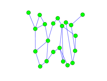
(a) Representative connected graph

(b) Representative disconnected graph

Figure 1: Representative graphs. The graph in Figure 1(a) is connected, while the one in Figure 1(b) is not. Yet, our intuition is that both graphs can perform much of their functions and meet most of their responsibilities even though they may not be able to meet all of them.

Our quest is to derive a metric for a graph (that is either connected or disconnected) that reports the inability of a graph to perform its functions. The inverse of this metric would report its ability to perform its functions, thusly how healthy the graph is. We intend for this metric to form the basis for a “game” where an attacker selects a graph component (either an edge or a vertex) for removal based on the amount of damage that the removal will cause to the graph. Additionally, the graph will be able to “repair” itself through the addition of new edges in between selected nodes that would result in a “less damaged” graph. The metric could be used as part of a “game” where an attacker and the graph alternated turns. The attacker could be given the equivalent of a some number of “bullets” to damage a graph and then the graph would be given the same number of repair opportunities to “repair” itself.

Section 2 presents related work by Albert, Jeong and Barabási, and Criado, Flores, et al., and Holme and Kim among others. A brief synopsis of relevant papers from these authors is given and how the metric that we intuit exists is different than that put forth by the authors. Section 3 presents the criteria that our metric must exhibit. Section 4 investigates how a collection of different metrics performs against a series of sample graphs. These proposed metrics are use against a small sample graph to triage candidate metrics. Once our metric is identified, we introduce a series of larger graphs and continue our investigation. Section 5 provides a summary analysis of Albert, Jeong and Barabási’s paper. Section 6 contains our conclusion. Appendix A contains a comparison of various graph related metrics applicable to both connected and disconnected graphs. Appendix B contains a more detailed analysis of Albert, Jeong and Barabási’s paper. Appendix C has a series of profiles that an attacker could use when seeking to damage a graph. These profiles contain techniques that can focus on either edges or vertices and then summarizes which profile is most effective.

2 Related work

Albert, Jeong and Barabási’s (AJB) paper [2] looks at the effect on the average (or expected) path length for a graph (specifically snapshots of the Internet and the WWW) when the highest degreed node (be it an Internet router, or a well connected HTML page) is removed from the graph. Within their context, the Internet is a graph where routers equate to nodes and communications links equate to edges. Also the WWW is a graph where pages equate to nodes and HTML links equate to edges. They proposed a tuple metric $(LCC,S,s)$ based on the proportion of the graph represented by the ratio of largest connected component $LCC$ to the entire graph $S$ and the mean size of all remaining fragments $s$ .

Klau and Weiskircher [15] formalized AJB’s idea into a two argument tuple $(S,s)$. Holme and Kim et al. [14] took AJB’s paper and expanded it by introducing the idea of using the average inverse path length (AIPL) as an approach to measure the vulnerability of a graph to different types of attacks. Crucitti, Latora, et al. [11] published a paper with the same title as AJB’s, dealing with the same general topic, but proposing a metric they called global efficiency. Their global efficiency is AIPL, but with a different name. Notetea and Pongor [20] proposed measuring the “robustness” of a network by computing the AIPL before and after a change is made to a graph under consideration. If the robustness of the graph is improved, then the change becomes permanent. If the robustness decreases then the change is reverted. Criado, Flores et al. in [10] propose to quantify the vulnerability of a graph based on the number of nodes, number of edges and the standard deviation of the degrees of the nodes. Ideas from these and other authors are expanded upon in the following sections.

2.1 Ideas from Albert, Jeong and Barabási

Equations 1 through 6 were derived from Albert, Jeong and Barabási [2], and are the basic definitions for the number of nodes $n$ in the graph at any point in time. At that point in time, there is a set of clusters $s$ in the graph. If the graph is connected then there is one cluster. In [2], the node with the highest degree is removed (along with its adjacent edges) and all values are computed again. $n$ starts at an initial value and is decremented at each time step until all nodes are disconnected.

Equation 3 is the number of clusters (components) in the set of clusters $c$. Equation 4 identifies the size of the largest connected component $LCC$ in $c$. Equation 5 is the ratio (percentage) of the size of $LCC$ to the current $n$. Equation 6 is the mean size of all the remaining clusters (i.e., less the $LCC$) in the graph. The minimal values of $s$ under differing conditions ($s$ $=f(n,LCC,m)$) are shown in Table 9.

$$n\stackrel{{\scriptstyle\mbox{\tiny{def}}}}{{=}}\mbox{ number of nodes in }G$$ (1)

$$c\stackrel{{\scriptstyle\mbox{\tiny{def}}}}{{=}}\mbox{ set of clusters in }G$$ (2)

$$m\stackrel{{\scriptstyle}}{{=}}\mathclose{\mid}c\mathclose{\mid}$$ (3)

$$LCC\stackrel{{\scriptstyle}}{{=}}max(\mid\mathclose{<}c\mathclose{>}\mathclose{\mid})$$ (4)

$$S\stackrel{{\scriptstyle}}{{=}}\frac{\mathclose{\mid}LCC\mathclose{\mid}~{}}{n}$$ (5)

$$s~{}\stackrel{{\scriptstyle}}{{=}}\frac{n-\mathclose{\mid}LCC\mathclose{\mid}~{}}{m-1}~{}$$ (6)

The various characteristics in equations 1 through 6 are subject to some mathematical constraints. These constraints are:

$$1\leq\mathclose{\mid}LCC\mathclose{\mid}~{}\leq n$$ (7)

$$m_{min}=\left\{\begin{array}[]{ll}1&\mbox{when }\mathclose{\mid}LCC\mathclose{\mid}~{}==n\\ 2&\mbox{otherwise}\end{array}\right.$$ (8)

$$m_{max}=\left\{\begin{array}[]{ll}1&\mbox{when }\mathclose{\mid}LCC\mathclose{\mid}~{}==n\\ n-LCC&\mbox{otherwise}\end{array}\right.$$ (9)

$$m_{min}\leq m\leq m_{max}$$ (10)

$$1\leq j\leq m$$ (11)

In addition to the mathematical constraints, there are a series of logical constraints. These constraints are:

1. $s$ $<\mathclose{\mid}LCC\mathclose{\mid}~{}$ (see Equation 6)

2. $S$ will always be in the range $\frac{1}{n}\leq S\leq 1$ (see Equation 5)

3. If $\mathclose{\mid}LCC\mathclose{\mid}$ == 1 then $\forall c:\mid c_{i}=1\Longrightarrow m=n$ meaning that anytime where $m==n$ and $\mathclose{\mid}LCC\mathclose{\mid}$ $\neq 1$ is a contradiction and can not happen.

4. If $\mathclose{\mid}LCC\mathclose{\mid}~{}==\frac{n}{2}\Longrightarrow m_{max}=\frac{n}{2}$ where $\forall c_{i}:\mathclose{\mid}c_{i}\mathclose{\mid}==1$.

5. If $\mathclose{\mid}LCC\mathclose{\mid}~{}==\frac{n}{j}\Longrightarrow m_{max}=\frac{n}{j}$ where $\forall c_{i}:\mathclose{\mid}c_{i}\mathclose{\mid}==1$.

6. If $\mathclose{\mid}LCC\mathclose{\mid}~{}==(n-1)\Longrightarrow m=2$.

Constraint 2 limits $\mathclose{\mid}LCC\mathclose{\mid}$ between $n$ and 1. The $\mathclose{\mid}LCC\mathclose{\mid}$   will equal $n$ when the graph is connected (i.e., the graph has not been fragmented). $LCC$ will equal 1 when the graph is totally disconnected (i.e., the graph is composed of only nodes and no edges). Equation 10 limits the number of fragments $m$ to between 1 and $n$. Equation 11 limits the number of fragments to the greater of 1 (when the graph is totally connected; i.e. one cluster) or $n$ (when the graph is totally disconnected). AJB were interested in the fraction $f$ of their graphs that had to be removed to cross a percolation threshold that would cause the graph to become severely fragmented. We are interested in the continuum of the graph’s performance while it is connected and after it is disconnected. The percolation threshold is of passing interest, while the ideas that they espouse serve as starting point for our investigation.

2.2 Ideas from Criado, Flores, et al.

Criado, Flores et al. in [10] propose to quantify the vulnerability of a graph based on the number of nodes, number of edges and the standard deviation of the degrees of the nodes. Perhaps most importantly, they define the attributes of a vulnerability function in terms of the graph.

Their definition is:

• Let $\mathcal{G}$ be the set of all possible graphs with a finite number of vertices. A vulnerability function $v$ is a function $v:\mathcal{G}\rightarrow[0,1]$  verifying the following properties:

  1. $v$ is invariant under isomorphisms.

  2. $v(G^{\prime})\leq v(G)$ if $G^{\prime}$ is obtained from $G$ by adding edges.

  3. $v(G)$ is computable in polynomial time with respect to the number of vertices of $G$.

The equation they present to meet their definitions is:

$$v^{**}(G)=\mbox{exp}\{\frac{\sigma}{n}+n-\mathclose{\mid}E\mathclose{\mid}-2+\frac{2}{n}\}$$ (12)

Supported by:

$$\sigma=\sqrt{\frac{1}{n}\sum_{i=1}^{n}(k_{i}-\frac{2\mathclose{\mid}E\mathclose{\mid}}{n})^{2}}$$ (13)

Equation 12 evaluates to the interval [0,1]. A value of 0 means that the graph is very robust (low vulnerability), while a value of 1 means that the graph is very vulnerable (not robust). Using equation 12 before and after a modification to a graph can be used as a way to measure what effect the change has had on the graph’s vulnerability. If the vulnerability increases, then probably the change should not be finalized. While their system of equations meets their requirements, the equations do not report the type of damage that we are interested in measuring. Their definition of the attributes of a metric are in harmony with our intuition.

2.3 Ideas from Holme and Kim

Holme and Kim in [14] looked at how an attacker could maximize the damage to a graph by following one of two approaches:

1. To remove the vertex with the highest initial degree (ID)

   $$c_{D}(v)=d(v)$$ (14)

2. Or, the vertex with the highest normalized in-betweenness centrality (IB)

   $$c_{B}(v)=\sum_{s\neq v\neq t\in V}\frac{\sigma_{st}(v)}{\sigma_{st}}$$ (15)

For these approaches, they allowed the attacker two different options. The options are:

1. To attack the graph (remove a vertex) based on the ordering of the vertices when a series of attacks started, or

2. To recompute ID and IB after a vertex has been removed.

This second option took into account that the characteristics of the graph change when a vertex is removed and therefore the ID and IB ordering would change. Recomputed ID and IB were called RD and RB respectively.

They used their ID, IB, RD and RB attack profiles on the hep-lat e-print archive, a snapshot of the Internet autonomous system connections over a 24 hour period and Erdös-Rényi random, Watts-Strogatz small-world, and Barabási-Albert scale-free graphs. They concluded that each of the different types of graphs respond (as in how the AIPL responds) differently and that the attacker should use the RB approach to maximize the impact as measured by AIPL.

Holme and Kim used AIPL as their metric to assess the functionality of the current graph. They did not use AIPL to assess how the most recent attack affected the graph’s ability to perform.

2.4 Ideas from Crucitti, Latora, Marchiori and Rapisarda

Crucitti et al. in [11] look at the behavior of a network (i.e., a graph that has a measurable flow along an edge) when a node or an edge is removed. Their premise is that the flow between nodes will always take the lowest cost path. In their models, each edge has a capacity and a tolerance factor. As edges/nodes are removed, the flow that was going through the removed component is spread out to other edges. The removal of a critical edge (high flow) and the redistribution of the flow through adjacent edges can result in a cascade of failures as the increased flow causes additional edges to reach saturation.

They investigated these phenomena for Erdös-Rényi random graphs and Barabási-Albert scale-free graphs using the same ideas of ID, IB, RD and RB as introduced in by Holme in [14]. Crucitti introduces the idea of global efficiency that has the same form and character as AIPL.

$$E(G)=\frac{1}{n(n-1)}\sum_{i\neq j\in V}\frac{1}{d_{ij}}$$ (16)

Crucitti computes global efficiency after a node or an edge is removed, but they do not compare the current efficiency versus a connected graph’s efficiency.

2.5 Ideas from Netotea and Pongor

Netotea and Pongor in [20] focus on the evolution of a graph towards a new organization that is more robust or efficient. Their definition of efficiency $E$ is AIPL and their definition of robustness $R$ is the ratio of the current efficiency $E_{t}$ divided by the the previous efficiency $R=\frac{E_{t}}{E}$.

Netotea and Pongor use a genetic algorithm that starts with a random graph (100 nodes and 120 edges) and mutates and crossovers the graph until it reaches a “steady state” condition. A steady state was achieved when the goals of $E$, $R$ and the maximum percentage of periphery nodes (those nodes with a degreeness of 1) was reached. $E_{t}$ was computed after either 1 or 5 of the highest betweenness nodes were removed.

Netotea and Pongor’s idea of robustness $R$ comes close to capturing our idea of a single number that measures the health of a graph. Health is the inverse of our idea of damage.

2.6 Ideas from others

Lee and Kim in [18] look at the effects of node and path failure on the Internet and report on the percentage of nodes that are required for disconnection. While they model failure of the graph, they do not report on how damaged the graph is when attempting to perform its functions.

Cohen et al. in [8] focus on the modeling the failure of the Internet when the most connected routers (highest degreed nodes) are removed. While they look towards quantifying the percolation value $p$ where the Internet and scale-free graphs become disconnected, they do not report on the graph’s ability to perform.

Newth and Ash in [21] look at cascading failures in a complex network. They extend the work of Crucitti et al. in [11] by manipulating their graph by: (1) adding a new edge, or (2) deleting an existing edge, or (3) changing one end of an existing edge. If the graph becomes disconnected during any of these operations, the change in rejected.

Beygelzimer et al. in [4] use AIPL as their metric for the robustness of a graph. They take an existing graph, rewire it using a number of different schemes and look at the robustness after each modification. They disallow any rewiring that would disconnect the graph.

Zio and Sansavini in [27] look at how the failure of a node or an edge may cause a failure in adjacent components as the load of the failed component cascades to its neighbors. These failures may be the result of random acts or targeted attacks. They do not use transfer of load as a metric of the damage done to the graph.

Lee et al. in [19] look at how the topology of the graph affects which type of attack profile would be most effective. They propose a new metric, called attack power to quantify the effect of any of their attack profiles. They measure damage to their graph using degree distribution, average path length and vertex cover. They enumerate some interesting attack profiles, but their approach does not address a disconnected graph. Klau and René Weiskircher in [15] (a chapter in [6]) provide a very nice survey of robustness and resilience metrics and ideas that have been advocated by various authors. None of the approaches provide a single unit-less value that describes the damage inflicted on a graph by the removal of an edge or node and the possible disconnection of the graph. Dekker in [12] introduces the idea of intelligence of a graph related to the quality of a sensor and the time delay associated with the data from the sensor. The intelligence of the graph starts to loose its meaning when the graph becomes disconnected. While the idea of intelligence in the graph is appealing to our sense that a graph can still perform when it is fragmented, Dekker’s metric does not speak to the total graph.

Ágoston et al. in [1] enumerate a series of attack profiles including:

1. Complete knockout — meaning the removal of a node and its adjacent edges,

2. Partial knockout — meaning the removal of a set of edges (but not all) adjacent to a node,

3. Attenuation — meaning that the amount of traffic that an edge can support is decreased, subsequently, the total cost of a path that uses that edge from a source node $s$ to a terminus node $t$ is increased,

4. Distributed knockout — meaning that a set of edges, not sharing a common node, are removed,

5. Distributed attenuation — meaning that the amount of traffic that the set of edges can support is decreased.

These attack profiles are used in simulated attacks on Escherichia coli and Saccharomyces cerevisiae transcriptional regulatory networks. Their conclusion is that multiple partial attacks causes more damage. Our interests are slightly different because edges in our network of DOs are really communications links vice edges that have a measurable capacity. DOs in our network can either send messages via these communications links or they can not. This difference in edge utilization and modeling eliminates the attenuation and distributed attenuation profiles. In our network, a DO exists or it does not and therefore all of its adjacent edges (communications links) are valid, or not. This approach matches Ágoston’s complete knockout profile. We view partial and distributed knockouts as being repeated application of removing single edges in our network.

Yin et al. in [26] take the ideas from Ágoston in [1] and apply them to scale-free and random graphs. Yin et al. apply weights to the edges in their graphs and use AIPL as a metric to quantify the effect of each attack profile. Their results confirm that scale-free networks are relatively immune to random attacks, but very sensitive to targeted attacks. While both random and targeted attacks on random graphs have relatively the same effect.

Lee et al. in [19] use the autonomic system (AS) connectivity graphs from National Laboratory for Applied Network Research as their test graph. Based on this graph, they apply weights to each of the edges in the graph based on the amount of traffic along that edge. They then focus on three different types of failures. Node failure where an AS is lost due to some sort of hardware failure (i.e., power supply failure, accidental or deliberate misconfiguration, etc.). Link failure where adjacent ASes are not able to communicate because of hardware failure (such as the cutting of a cable), or electronic failure (such as DNS hacking, routing table poisoning, etc.). Path failure including DoS and routing table loops, resulting in a flooding of the path with packets to the extent that the communications links are unusable. Lee et al. then create different attack profiles based on these types of failures. Their attack profiles are:

1. Random AS attack — randomly choose an AS and and remove it,

2. Min-degree AS attack — order the ASes by their degree connectivity and then start removing them from low degree to high degree order,

3. Max-degree AS attack — order the ASes by the degree connectivity and then start removing them from high degree to low degree order,

4. Random edge attack — randomly choose an edge and remove it,

5. Min-weight edge attack — order the edges by their weight and then start removing them from low weight to high weight order,

6. Max-weight edge attack — order the edges by their weight and then start removing them from high weight to low weight order,

7. Random path attack — randomly choose a path and remove it,

8. Max-weight edge attack — order all paths by weight and then remove paths in order from heaviest to lightest, and

9. Max-length path attack — order all paths by length and then remove paths in order from longest to shortest.

After each attack, the effect on the graph is quantified by a metric they labeled as “attack power” Attack power reports the effect of each attack on the number of components that fail in the system. We treat Lee’s path failure as a limited case of our edge failure (see Section C.2.2) . Path failure is based on the path at the start of the attack where the path meets some sort of criteria and then a series of edges are removed based on these criteria. The limitation is that the set of criteria used to identify the path in the first place, may not be valid after the removal of the first edge in the path. We select an edge based on some criteria, remove the edge and then reevaluate the entire graph to select the next edge. We do not base future actions on information that may be stale or obsolete.

Latora et al. in [17] look at the vulnerability of complex networks to three different attack profiles and then provide a method to reduce the vulnerability of the network by the addition of edges between selected nodes. Their attack profiles are: loss of a single cable connection (loss of an edge), loss of a single Internet router (loss of a single node) and loss of two Internet routers (loss of two nodes). They assume that for the system $S$ there exists a performance metric $\Phi[S]>0$ that characterizes the performance of the graph and that this metric increases in value when the graph is damaged $D$. Therefore

$$V[S,D]=\frac{\Phi[S]-W[S,D]}{\Phi[S]}$$ (17)

Where $W[S,D]=\Phi[D(S,d^{*})]$ is the worst possible damage that can happen to the graph based on a specific attack profile. They use $V[S,D]$ as a metric to quantify the efficacy of an attack. The same metric is used to evaluate the effect of adding a communications link (an edge) between any two nodes in order to improve (i.e., reduce the vulnerability) of the system. Our approach is different in that we we are explicit about the metric that we will use to measure the “performance” of the graph and we are currently focusing on attacking the graph vice repairing it. Our approach could be used to evaluate graph repair alternatives.

3 An alternative approach

After looking at the different approaches in Section 2 and thinking about what it is that the damage metric is trying to capture, we do not feel that individually any of them fit the bill.

The attributes of the damage metric should be:

1. Different fragmentation cases should result in different numerical value,

2. Test cases where the size of the fragments have been scaled, and the entire graph (for instance, increased by a factor of 10 or 0.1) should result in the same value

3. The value should be useful without additional information about the graph (i.e., the metric is graph independent and does not require knowledge of the graph in a different state),

4. The metric should be unitless. The approach and equations from AJB’s paper [2] have some function of $node$. The units of $S$ or $\mathclose{\mid}LCC\mathclose{\mid}$ and $s$ is $nodes$. $F_{score}$ (see Equation 21) and the generalized $F_{\beta}$ (see Equation 22) metrics have units of $nodes$. Geometric (see Equation 23) and quadratic mean (see Equation 24) and ratio ($s$ $/$$S$ ) are unit-less and therefore attractive.

The desire/need to have a unit-less and scale-free description of the fragmentation and damage of a graph points to using a different type of metric. One that appears popular is based on the average inverse average path length (AIPL) (see Equation 39) . There are a couple of variations on Equation 39, such as Equation 18 from [20] and Equation 19 from [11]. Equation 18 is applicable to a graph that has directed edges and permits self loops. Equation 19 is applicable to a graph that has directed edges and does not permit self loops.

$$E(G)=\frac{1}{n(n+1)}\sum_{i\neq j\in V}\frac{1}{d_{ij}}$$ (18)

$$E(G)=\frac{1}{n(n-1)}\sum_{i\neq j\in V}\frac{1}{d_{ij}}$$ (19)

AIPL equations are used to compute the AIPL between any pair of nodes in a graph, even if the graph is disconnected. Use of the AIPL can be counter intuitive, in that a larger AIPL is better than a smaller AIPL because a smaller AIPL means that the average path length is increasing.

At the core of the $Damage(G)$ metric is the ratio of two AIPLs. One of the damaged/fragmented graph and the other an unfragmented artificial graph.

$$Damage(G)=1-\frac{L(G_{fragmented})^{-1}}{L(G_{unfragmented})^{-1}}$$ (20)

The unfragmented artificial graph is constructed by sorting the original graph fragments by their size and repeatedly connecting the nodes of two largest fragments with the highest centrality value (see Equation 29) until the graph is connected. Conceptually, the artificial graph could have been existed in the fragmented graph’s past and the current fragmented graph is the result from losing edges. The edges could have been lost due to error or attack.

4 Comparison and evaluation of various metrics

4.1 Small test case

We create a small graph with 21 nodes and 27 edges (see Figure 2) , and use it to show the effects on “classical” graph metrics by using different attack profiles. Damage will be inflected on the graph by targeting either the edge ($A_{E,*}$ ) or the vertex ($A_{V,*}$ ) based on its betweenness centrality measurement. The betweenness centrality measurement is a count (or normalized value) of the number of geodesic paths that use either an edge or a vertex, hence edge or vertex centrality to the graph.

For $A_{E,*}$  or $A_{V,*}$ , the appropriate centrality measurement is computed and the component (edge or vertex as applicable) is removed from the graph. Various graph metrics are computed and reported after each removal. This targeted attack is repeated until the graph becomes disconnected. After targeting the edges, the graph will be restored to its initial condition prior to targeting the vertices.

Removing graph components (either an edge or a vertex) may result in the graph becoming disconnected, or fragmented. Sometimes this fragmentation will result in a graph that is divided in half and whose $LCC$ is approximately the same size as the non $LCC$. A different choice in which component to remove (a different attack criteria), might result in a graph whose $LCC$ contains all the remaining edges and all but one node.

Figure 2: Small test graph used to show the effects of different attack profiles. The graph has 21 nodes and 27 edges. It clearly shows 2 groupings of nodes that are connected by 2 separate sets of edges.

4.1.1 Removal of vertices

The effect of the $A_{V,H}$  profile is tabulated in Table 1 and shown diagrammatically in Figure 3. Table 1 lists selected “classic” graph metric values and some are invalid after removing the second vertex. Prior to the first removal, the centrality measurement for all vertices is computed. The vertex with the highest value is then removed and all centrality values are recomputed so that the new highest valued vertex can be identified. In Figure 3, each vertex is labeled with its centrality value and the one with the highest value is drawn in red.

The graph is disconnected after removing two vertices. Removing the vertices or edges with the highest centrality measurement results in a disconnected graph after two removals, but the choice of with type of component to remove results in two different graphs (compare Figure 3 and Figure 4).

Metric name	Original values	After removal of the vertex with the 69 centrality measurement	After removal of the vertex with the 98 centrality measurement
Highest vertex centrality	69	98	28
APL	3.86	4.54	—
AIPL	0.38	0.35	0.24
Clustering coefficient	0.12	0.16	0.12
Diameter	10.00	11.00	—
Eccentricity	10.00	11.00	—
Radius	1.00	1.00	—

Table 1: Effects of an $A_{V,H}$  attack profile on the sample graph. Various “classic” graph values are computed using the original graph, including the vertex centrality of all vertices. The vertex with the highest centrality is then removed (see Figure 3(b)) and the values are recomputed. Again, the vertex with the highest centrality is removed (see Figure 3(c)) and values are computed. The marker — is used to indicate that the graph metric is not computable because the graph is disconnected.

(a) Original graph labeled with vertex betweenness values

(b) Identifying and labeling first highest valued vertex

(c) Identifying and labeling new highest valued vertex after removing initial highest valued vertex

(d) The graph after removing two vertices

Figure 3: Damage to a graph by the $A_{V,H}$  profile. Each vertex in the original graph is labeled with its centrality value (see Figure 4(a)) . The vertex with the highest centrality measurement is selected and highlighted prior to its removal (see Figure 3(b)) . After the removal of the first vertex, all vertex centrality values are recomputed and again the vertex with the highest value is selected for removal (see Figure 3(c)) . The graph is disconnected after the removal of the second vertex (see Figure 3(d)) .

4.1.2 Removal of edges

The effect of the $A_{E,H}$  profile is tabulated in Table 2 and shown diagrammatically in Figure 4. Table 2 lists selected “classic” graph metric values and some are non valid after removing the second edge. Prior to the first removal, the centrality measurement for all edges is computed. The edge with the highest value is then removed and all centrality values are recomputed so that the new highest valued edge can be identified. Note that this is different than an attack on a path because a path based attack does not recompute a new set of paths after each removal. In Figure 4, each edge is labeled with its centrality value and the one with the highest value is drawn with a wide red stroke.

The graph is disconnected after removing two edges. Removing the vertices or edges with the highest centrality measurement results in a disconnected graph after two removals, but the choice of with type of component to remove results in two different graphs (compare Figure 3 and Figure 4).

Metric name	Original values	After removal of the edge with the 59 centrality measurement	After removal of the edge with the 110 centrality measurement
Highest edge centrality	59	110	18
APL	3.86	4.34	—
AIPL	0.38	0.36	0.26
Clustering coefficient	0.12	0.13	0.13
Diameter	10.00	11.00	—
Eccentricity	10.00	11.00	—
Radius	1.00	1.00	—

Table 2: Effects of an $A_{E,H}$  attack profile on the sample graph. Various “classic” graph values are computed using the original graph, including the edge centrality of all edges. The edge with the highest centrality is then removed (see Figure 4(b)) and the values are recomputed. Again, the edge with the highest centrality is removed (see Figure 4(c)) and values are computed. The marker — is used to indicate that the graph metric is not computable because the graph is disconnected.

(a) Original graph labeled with edge betweenness values

(b) Identifying and labeling first highest centrality valued edge

(c) Identifying and labeling new highest centrality valued edge after removing initial highest valued edge

(d) The graph after removing two edges

Figure 4: Damage to a graph by the $A_{E,H}$  profile. Each edge in the original graph is labeled with its edge centrality value (see Figure 4(a)) . The edge with the highest centrality measurement is selected and highlighted prior to its removal (see Figure 4(b)) . After the removal of the first edge, all edge centrality values are recomputed and again the edge with the highest value is selected for removal (see Figure 4(c)) . The graph is disconnected after the removal of the second edge (see Figure 4(d)) .

4.1.3 Comparing $A_{E,H}$  and $A_{V,H}$  profiles

Both the $A_{E,H}$  and the $A_{V,H}$  profiles result in a disconnected graph after to removals. But the two profiles result in different graphs at time point of disconnection (compare Figure 3(d) and Figure 4(d)).

4.2 A change in notation

Figure 2 is small and sparse enough that it is practical to draw and label the complete graph and still be able to understand its structure. As graphs get larger, and more interesting it is not practical to draw and label every component. Therefore, we introduce a different notation style that is more in keeping with the aspects of the graph that are if interest to our research.

We are interested in how the graph functions, its connectivity as it becomes more and more fragmented. The internal connectivity (how many edges are in a fragment) is of less interest than the fact that the graph is fragmented, and that the numbers and relative sizes of these fragments can be used as a metric to describe how well the fragmented graph “operates” when compared to the unfragmented graph.

Specific graph instances will have names such as 90,10 whose $\mathclose{\mid}LCC\mathclose{\mid}$ and number and size of any fragments are shown in Table 3. Tables 4.3 through 4.3 provide notational diagrams of the graph instances.

4.3 Larger test cases

A series of test cases were constructed to exercise the different approaches proposed by Albert, Jeong and Barabási and ourselves. Each test case consists of some number of fragments (a.k.a., components) between 1 and 11. The test cases are intuitively ordered from least to most damaged. The test cases are described numerically in Table 3, and shown diagrammatically in Tables 4.3 through 4.3.

Name	$\mathclose{\mid}LCC\mathclose{\mid}$	Frag. 2	Frag. 3	Frag. 4	Frag. 5	Frag. 6	Frag. 7	Frag. 8	Frag. 9	Frag. 10	Frag. 11
100	100	—	—	—	—	—	—	—	—	—	—
90,10	90	10	—	—	—	—	—	—	—	—	—
90…1	90	1	1	1	1	1	1	1	1	1	1
80…2	80	2	2	2	2	2	2	2	2	2	2
50,50	50	50	—	—	—	—	—	—	—	—	—
50,49,1	50	49	1	—	—	—	—	—	—	—	—
50,40,10	50	40	10	—	—	—	—	—	—	—	—
50,30,10,10	50	30	10	10	—	—	—	—	—	—	—
50…5	50	5	5	5	5	5	5	5	5	5	5
20…20	20	20	20	20	20	—	—	—	—	—	—
16…1	16	15	14	13	10	9	8	7	4	3	1
10…10	10	10	10	10	10	10	10	10	10	10	—
10…9	10	9	9	9	9	9	9	9	9	9	9
1…1	1	1	1	1	1	1	1	1	1	1	1

Table 3: A collection of connected and disconnected graphs used as test cases. This is a set of graphs (some of which are connected and others that are not) used to test various metrics and report how well the metric matches our intuition of damage to the graph. Each graph has 100 nodes. The test cases are ordered by $\mathclose{\mid}LCC\mathclose{\mid}$ .

Name	$s$	$Damage(G)$
100	NaN	0.00
90,10	10.00	0.14
90…1	1.00	0.16
80…2	2.00	0.31
50,50	50.00	0.39
50,49,1	25.00	0.40
50,40,10	25.00	0.46
50,30,10,10	16.67	0.52
50…5	5.00	0.64
20…20	20.00	0.66
16…1	8.40	0.78
10…10	10.00	0.81
10…9	9.00	0.82
1…1	1.00	1.00

Table 4: Comparing AJB’s raw $s$ to our proposed metric for the test graphs. Raw $s$ and $Damage(G)$ are being evaluated as surrogates for the “health” of the graph. A healthy graph would have a value close to 0, while a totally disconnected graph would have a value of 1. Normalizing $s$ to either the size of the graph, or to $\mathclose{\mid}LCC\mathclose{\mid}$ does not meet these desired criteria.

& 100  diagram, $s~{}=NaN$ , $Damage(G)=0.00$ 90,10  diagram, $s~{}=10.00$ , $Damage(G)=0.14$ 90…1  diagram, $s~{}=1.00$ , $Damage(G)=0.16$ 80…2  diagram, $s~{}=2.00$ , $Damage(G)=0.31$

Table 5: Notional diagrams for test cases 100 , 90,10 , 90…1 and 80…2 . The entire graph is contained with in the square. The LCC is represented by the large inner circle. While the smaller fragments are represented by the outer circles. Within each square, the circles represent the relative sizes of the different fragments.

Table 6: Notional diagrams for test cases 50,50 , 50,49,1 , 50,40,10 and 50,30,10,10 . The entire graph is contained with in the square. The LCC is represented by the large inner circle. While the smaller fragments are represented by the outer circles. Within each square, the circles represent the relative sizes of the different fragments.

& 50,50  diagram, $s~{}=50.00$ , $Damage(G)=0.39$ 50,49,1  diagram, $s~{}=25.00$ , $Damage(G)=0.40$ 50,40,10  diagram, $s~{}=25.00$ , $Damage(G)=0.46$ 50,30,10,10  diagram, $s~{}=16.67$ , $Damage(G)=0.52$

Table 7: Notional diagrams for test cases 50…5 , 20…20 , 16…1 and 10…10 . The entire graph is contained with in the square. The LCC is represented by the large inner circle. While the smaller fragments are represented by the outer circles. Within each square, the circles represent the relative sizes of the different fragments.

& 50…5  diagram, $s~{}=5.00$ , $Damage(G)=0.64$ 20…20  diagram, $s~{}=20.00$ , $Damage(G)=0.66$ 16…1  diagram, $s~{}=8.40$ , $Damage(G)=0.78$ 10…10  diagram, $s~{}=10.00$ , $Damage(G)=0.81$

Table 8: Notional diagrams for test cases 10…9 and 1…1 . The entire graph is contained with in the square. The LCC is represented by the large inner circle. While the smaller fragments are represented by the outer circles. Within each square, the circles represent the relative sizes of the different fragments.

& 10…9  diagram, $s~{}=9.00$ , $Damage(G)=0.82$ 1…1  diagram, $s~{}=1.00$ , $Damage(G)=1.00$

4.4 Comparison equations

Now that we have the basic definitions and constraints out of the way, we can begin to look at how AJB’s $S$ and $s$ will be evaluated. A set of equations was selected that seemed like they might be of use. The set includes:

1. The median value of all the fragments, except the $LCC$.

2. The average size of all the fragments, except the $LCC$.

3. The standard deviation of all the fragments, except the $LCC$.

4. The harmonic mean of all the fragments, except the $LCC$.

5. The geometric mean of all the fragments, except the $LCC$.

6. A variation on the information retrieval (IR) metric $F_{score}$ (see Equation 21) (a 2 value harmonic mean). We selected $F_{score}$ because it had been used in other applications and we thought that it might be useful. In the IR world, $F_{score}$ traditionally operates on the values of precision and recall. For the purposes of analysis $S$ was treated as precision and $s$ was treated as recall.

   $$F_{score}=\frac{2*\textrm{precision}*\textrm{recall}}{\textrm{precision}+\textrm{recall}}$$ (21)

7. A generalized $F_{\beta}$ (see Equation 22) metric that incorporates a value $\beta$ that is used to weight precision relative to recall.

   $$F_{\beta}=(1+\beta^{2})\frac{\textrm{precision}*\textrm{recall}}{\beta^{2}\textrm{precision}+\textrm{recall}}$$ (22)

8. A simple arithmetic mean of $S$ and $s$ .

9. A geometric mean of $S$ and $s$  (see Equation 23) .

   $$G=\sqrt[n]{x_{1}x_{2}...x_{n}}$$ (23)

10. A quadratic mean of $S$ and $s$  (see Equation 24) .

    $$Q_{rms}=\sqrt{\frac{x_{1}^{2}+x_{2}^{2}+...+x_{n}^{2}}{n}}$$ (24)

11. Ratio of $s$ to $S$ .

12. $S$ raised to the $s$ power.

13. $s$ raised to the $S$ power.

In equations 21 through 24, $x_{1}=S$ and $x_{2}=s$.

5 Analysis

The interaction between $S$ , $LLC$ and $s$ is of interest and is summarized in Table 9. Various cells in Table 9 are have different colors and color is significant. Cells that are filled with cyan  violate some basic mathematical operation. Cells that are filled with orange  violate some some logical restriction on $LCC$ (see Constraint 7) . Cells that are filled with red  violate some logical restriction on $m$ (see Constraint 3) . There may be cases when a combination of $j$, $m$, $S$ , $LLC$ and $s$ violates more than one constraint, in those cases the fill color will be chosen at random. Cells that are not filled, do not violate any constraints. There is a limited range of values for $m$ and $\mathclose{\mid}LCC\mathclose{\mid}$   that do not violate some sort of mathematical or logical constraint when attempting to compute $s$ . These limits are in keeping with the values computed in AJB’s paper.

The test cases from Table 3 were subjected to a series of mathematical investigations looking to identify and quantify a metric that was near 0 for “undamaged” graphs and near 1 for “damaged” ones. Table 10 shows the various mean and standard deviation values for the test cases. These approaches produced values that had no discernible relationship to their state of damage. Table 11 showed some useful information, but each of these more sophisticated approaches, had some sort of “hump” or “swale” in the computed values. Values produced by using these approaches would initially trend in the right direction (from low to high) as the case numbers increased, but then the values would change direction and start to go the other way. Some of the exponentiation cases, created values that were too large for the computer to handle reasonably. While these computational limitations could be overcome, there does not seem to be any reason to expend the effort to do so when the data that was available was not well behaved. None of the approaches in Tables 10 and 11 showed the desired property of continuous directed change.

The investigation into a unit-less metric for assessing the “damage” inflicted upon a graph by fragmentation, led to writing an R script that could produce three different types of graphs; random, small world and scale free. These graph types were selected because they are felt to represent approximately the extremes of the fundamental graph types.

The R script takes as an a argument the fragments that make up the test case (see Table 3) . Two graphs are created based on the fragments. The first graph is a simple connected graph whose size is equal to the sum of the fragments. The second graph is a simple disconnected graph whose size is equal to the sum of the fragments.

The average inverse path length (AIPL) (see Equation 39) for the two graphs is computed and then the ratio of the AIPLs is reported. The hoped for behavior (a value near zero when the graph is not too damaged, and near unity when severely damage) is exhibited by the ratio of the AIPLs (see Table 12) .

The ratio of the AIPLs metric for the test cases does range from 1.0 to 0.0 (see Table 12) fitting our intuition. Now the question becomes, does that metric continue (within reasonable bounds) as the size of the graph changes, this is in keeping with the desirable behavior of the metric as listed in section 3. The base size of the graph was increased by factors of 2, 4, 8 and 10, the ratio was computed and reported (see Table 13) . Data in Table 13 shows the metric starts at 1.0 for a non-fragmented graph and decreases towards 0.00 as the graph becomes more fragmented and $\mathclose{\mid}LCC\mathclose{\mid}$ becomes smaller. Data in the table for totally fragmented graphs does not reach 0.000 as the graph becomes larger possibly because the round offs when computing all the paths and their inverses start to accumulate. Where the expected value should be 0.000, it is in fact 0.0. Computing all shortest paths in a graph using the Floyd-Warshall algorithm can take $\Theta(V^{3})$ time [9], so larger graphs were not fully analyzed.

		$\mid LCC\mid$
		1	$\frac{n}{2}$	$\frac{n}{j}$	$n-1$	$n$
$m$	1	$\frac{n-1}{1-1}=undef$	$\frac{n-\frac{n}{2}}{1-1}=undef$	$\frac{n-\frac{n}{j}}{1-1}=undef$	$\frac{n-(n-1)}{1-1}=undef$	$\frac{n-n}{1-1}=undef$
	$2$	$\frac{n-1}{2-1}=n-1\mbox{ (C\ref{cont:5})}\pagecolor{orange}$	$\frac{n-\frac{n}{2}}{2-1}=\frac{n}{2}$	$\frac{n-\frac{n}{j}}{2-1}=n(1-\frac{1}{j})$	$\frac{n-(n-1)}{2-1}=1$	$\frac{n-n}{2-1}=0$
	$\frac{n}{2}$	$\approx 2\mbox{ (E\ref{equ:3-3})}\mbox{ (C\ref{cont:1})}\pagecolor{orange}$	$\approx 1\mbox{ (E\ref{equ:3-4})}$	$\approx 2-\frac{2}{j}\mbox{ (E\ref{equ:3-5})}$	$\frac{2}{n}\mbox{ (E\ref{equ:3-6})}\mbox{ (C\ref{cont:4})}\pagecolor{orange}$	$\frac{n-n}{\frac{n}{2}-1}=0$
	$\frac{n}{j}$	$\approx j\mbox{ (E\ref{equ:4-3})}\mbox{ (C\ref{cont:1})}\pagecolor{orange}$	$\approx\frac{j}{2}\mbox{ (E\ref{equ:4-4})}$	$\approx j-1\mbox{ (E\ref{equ:4-5})}$	$=\frac{j}{n}\mbox{ (E\ref{equ:4-6})}\mbox{ (C\ref{cont:4})}\pagecolor{orange}$	$\frac{n-n}{\frac{n}{j}-1}=0$
	$n-1$	$\approx 1\mbox{ (E\ref{equ:5-3})}\mbox{ (C\ref{cont:1})}\pagecolor{orange}$	$\approx\frac{1}{2}\mbox{ (E\ref{equ:5-4})}\mbox{ (C\ref{cont:2})}\pagecolor{orange}$	$\approx 1-\frac{1}{j}\mbox{ (E\ref{equ:5-5})}\mbox{ (C\ref{cont:2})}\pagecolor{orange}$	$\approx\frac{1}{n}\mbox{ (E\ref{equ:5-6})}\mbox{ (C\ref{cont:4})}\pagecolor{orange}$	$\frac{n-n}{(n-1)-1}=0$
$n$	$\frac{n-1}{n-1}=1$	$\approx\frac{1}{2}\mbox{ (E\ref{equ:6-4})}\mbox{ (C\ref{cont:2})}\pagecolor{orange}$	$\approx 1-\frac{1}{j}\mbox{ (E\ref{equ:6-5})}\mbox{ (C\ref{cont:2})}\pagecolor{orange}$	$\approx\frac{1}{n}\mbox{ (E\ref{equ:6-6})}\mbox{ (C\ref{cont:4})}\pagecolor{orange}$	$\frac{n-n}{n-1}=0$

Table 9: Analysis of $s$ based on possible values of $\mathclose{\mid}LCC\mathclose{\mid}$   and $m$. $s~{}\stackrel{{\scriptstyle}}{{=}}\frac{n-\mathclose{\mid}LCC\mathclose{\mid}~{}}{m-1}$ is the average size of all fragments in the graph, less the $LCC$. The table summarizes the lower limit on $s$ based on the maximum number of fragments $m$ there can be in the graph based on $\mathclose{\mid}LCC\mathclose{\mid}$ . Where the value in the cell is not obvious (i.e., how it was derived, what assumptions were made, etc.), the (E#) refers to a set of equations that show how the value was obtained. In some cells there is a constraint logical violation. These constraint violations are shown as (C#).

						Standard	Harmonic	Geometric
Name	S	s	m	Median	Mean	Deviation	Mean	Mean
100	100	NaN	1	100.00	100.00	NA	100.00	100.00
90,10	90	10	2	50.00	50.00	56.57	18.00	30.00
90…1	90	1	11	1.00	9.09	26.83	1.10	1.51
80…2	80	2	11	2.00	9.09	23.52	2.19	2.80
50,50	50	50	2	50.00	50.00	0.00	50.00	50.00
50,49,1	50	25	3	49.00	33.33	28.01	2.88	13.48
50,40,10	50	25	3	40.00	33.33	20.82	20.69	27.14
50,30,10,10	50	17	4	20.00	25.00	19.15	15.79	19.68
50…5	50	5	11	5.00	9.09	13.57	5.45	6.16
20…20	20	20	5	20.00	20.00	0.00	20.00	20.00
16…1	16	8	11	9.00	9.09	5.07	4.70	7.19
10…10	10	10	10	10.00	10.00	0.00	10.00	10.00
10…9	10	9	11	9.00	9.09	0.30	9.08	9.09
1…1	1	1	100	1.00	1.00	0.00	1.00	1.00

Table 10: Simple and standard statistical approaches applied to $S$ and the set of all fragments less the $LCC$. The hoped for behavior of the metrics is to be a “good” value (approximately 0) for the low numbered cases and a “bad” value (approximately 1) for the high numbered cases. The simple statistical approaches did not produce the type of hoped for behavior.

	$F_{score}$	$F_{\beta}$	Arithmetic	Geometric	Quadratic	Ratio
Name		$\beta=0.5$	Mean	Mean	Mean	(s/S)	$\log{(S^{s})}$	$\log{(s^{S})}$
100	NaN	NaN	100.00	100.00	100.00	NaN	NaN	NaN
90,10	18.00	34.62	50.00	30.00	64.03	0.11	45.00	207.23
90…1	1.98	4.79	9.09	1.51	27.15	0.01	4.50	0.00
80…2	3.90	9.09	9.09	2.80	24.20	0.03	8.76	55.45
50,50	50.00	50.00	50.00	50.00	50.00	1.00	195.60	195.60
50,49,1	33.33	41.67	33.33	13.48	40.42	0.50	97.80	160.94
50,40,10	33.33	41.67	33.33	27.14	37.42	0.50	97.80	160.94
50,30,10,10	25.00	35.71	25.00	19.68	30.00	0.33	65.20	140.67
50…5	9.09	17.86	9.09	6.16	15.81	0.10	19.56	80.47
20…20	20.00	20.00	20.00	20.00	20.00	1.00	59.91	59.91
16…1	11.02	13.55	9.09	7.19	10.30	0.53	23.29	34.05
10…10	10.00	10.00	10.00	10.00	10.00	1.00	23.03	23.03
10…9	9.47	9.78	9.09	9.09	9.10	0.90	20.72	21.97
1…1	1.00	1.00	1.00	1.00	1.00	1.00	0.00	0.00

Table 11: Slightly more sophisticated statistical approaches applied to $S$ and the set of all fragments less the $LCC$. Equations 21 through 24 were applied to $S$ and $s$ where $x_{1}=S$ and $x_{2}=s$. For all the test cases, the computed values had a “hump” and a “swale” minimizing their utility as a metric for the “fitness” or “damage” of a graph. The hoped for behavior of the metric is to be a “good” value (something approaching 0.0) for the low numbered cases and a “bad” value (something approaching 1.0) for the high numbered cases. The ratio of $s$ and $S$ are not particularly usable, and most of the $s$ and $S$ exponentiations result in hugely large numbers that do not appear to be very enlightening.

	Albert, Jeong and Barabási			$Damage(G)$
					Small	Scale
Name	S	s	m	Random	World	Free
100	100	NaN	1	0.000	0.000	0.000
90,10	90	10	2	0.181	0.106	0.140
90…1	90	1	11	0.191	0.135	0.159
80…2	80	2	11	0.357	0.265	0.308
50,50	50	50	2	0.506	0.275	0.387
50,49,1	50	25	3	0.515	0.285	0.395
50,40,10	50	25	3	0.585	0.345	0.459
50,30,10,10	50	17	4	0.645	0.407	0.520
50…5	50	5	11	0.733	0.573	0.638
20…20	20	20	5	0.803	0.536	0.658
16…1	16	8	11	0.890	0.692	0.778
10…10	10	10	10	0.907	0.712	0.807
10…9	10	9	11	0.917	0.741	0.822
1…1	1	1	100	1.000	1.000	1.000

Table 12: Application of proposed damage metric to the test case graphs. The hoped for behavior of the metrics is to be a “good” value (approximately 0) for the low numbered cases and a “bad” value (approximately 1) for the high numbered cases. AJB in [2] based their analysis on graph information that they obtained on Internet and HTTP connectivity. Based on the statistics for those graphs, they constructed exponential (random degree distribution) and scale-free graphs with the same notional properties.

	200 nodes			400 nodes
Base	Ran-	Small	Scale	Ran-	Small	Scale
Case	dom	World	Free	dom	World	Free
100	0.000	0.000	0.000	0.000	0.000	0.000
90,10	0.181	0.080	0.149	0.181	0.131	0.154
90…1	0.190	0.115	0.167	0.190	0.167	0.168
80…2	0.359	0.202	0.311	0.357	0.227	0.320
50,50	0.505	0.194	0.409	0.501	0.206	0.444
50,49,1	0.514	0.205	0.417	0.511	0.215	0.454
50,40,10	0.584	0.266	0.482	0.582	0.250	0.516
50,30,10,10	0.644	0.334	0.540	0.642	0.317	0.573
50…5	0.729	0.481	0.647	0.726	0.455	0.666
20…20	0.804	0.469	0.682	0.802	0.418	0.719
16…1	0.886	0.608	0.779	0.886	0.563	0.807
10…10	0.902	0.626	0.798	0.902	0.578	0.823
10…9	0.911	0.649	0.812	0.911	0.597	0.830
1…1	0.994	0.974	0.975	0.993	0.939	0.970
	800 nodes			1000 nodes
Base	Ran-	Small	Scale	Ran-	Small	Scale
Case	dom	World	Free	dom	World	Free
100	0.000	0.000	0.000	0.000	0.000	0.000
90,10	0.180	0.044	0.161	0.180	0.124	0.161
90…1	0.189	0.073	0.174	0.189	0.148	0.173
80…2	0.356	0.228	0.328	0.356	0.307	0.330
50,50	0.501	0.350	0.434	0.501	0.330	0.444
50,49,1	0.510	0.362	0.444	0.510	0.333	0.454
50,40,10	0.581	0.395	0.512	0.581	0.416	0.520
50,30,10,10	0.641	0.436	0.575	0.641	0.456	0.582
50…5	0.726	0.538	0.667	0.726	0.541	0.675
20…20	0.801	0.495	0.733	0.801	0.574	0.741
16…1	0.885	0.609	0.824	0.885	0.637	0.829
10…10	0.901	0.621	0.841	0.901	0.656	0.847
10…9	0.910	0.650	0.852	0.910	0.668	0.856
1…1	0.991	0.907	0.970	0.991	0.901	0.970

Table 13: Results of testing the proposed metric on larger graphs. The base case of a 100 node graph was increased by factors of 2, 4, 8 and 10 to ensure that the metric continued to perform correctly. In all cases, the ratio worked intuitively, starting at 0.0 for a non-fragmented graph and increasing towards 1.0 for a totally fragmented graph. Some of the fully fragmented graphs, did not reach 1.000 possibly due to round off errors in the computations. Those fully fragmented graphs that did not reach 1.000 did reach 1.0 as expected.

6 Conclusion

Considerable time was spent examining the equation Albert, Jeong and Barabási $s~{}\stackrel{{\scriptstyle}}{{=}}\frac{n-\mathclose{\mid}LCC\mathclose{\mid}~{}}{m-1}$ from [2] to see how it could be used to quantify the “damage” to a graph when the graph becomes fragmented. This investigation was spurred on by the equation’s use in [2, 6] and the belief that there was more information there that could be of use. The equation was analyzed and limits (both mathematical and logical) were identified. These limits fit nicely with the graphs in both references.

Because of the limitations experienced using the tuple ($s$ , $m$, $S$ ) from AJB and the desire to have a unit-less metric that reflects the efficiency of the graph; a different approach was identified. Netotea and Pongor in [20] and Crucitti et al. in [11] proposed the use of the average inverse path length (AIPL) as a way of quantifying the efficiency of a graph. We used the equations from Crucitti to compute the AIPL of a connected graph that is equal to the sum of all the fragments and the original disconnected graph consisting of the fragments. A ratio was computed using these AIPLs. This ratio has the desired effect of being: (1) unit-less, (2) independent of graph size, and (3) does not require a priori knowledge of the graph.

The ratio of the average inverse path lengths of a connected and a disconnected graph can be used as a metric about the health of a graph. The damage (i.e., the converse of health) of a fragmented graph can be computed using $Damage(G)=1-\frac{L(G_{fragmented})^{-1}}{L(G_{unfragmented})^{-1}}$.

7 Acknowledgment

This work supported in part by the NSF, Project 370161.

Appendix A Comparison of connected and disconnected graph metrics

Within this paper the following terms and ideas are used:

1. A graph $G(V,E)$ is an ordered pair of disjoint sets ($V$,$E$) such that $E$ is a subset of $V^{2}$ of the unordered pairs of $V$ [5].

2. The terms vertex and node are used interchangeably and mean the same thing.

3. The term connected means that there is a series edges between any arbitrary nodes source s and terminus t that can be used to get from node s to t[5]. A graph is disconnected when nodes s and t cannot be reached by any series of edges.

4. The term directed means that the edge connecting nodes s and t is unidirectional. t is an immediate neighbor to s because they are separated by one edge and it takes more than one edge for t to reach s.

5. The term undirected means that the edge connecting nodes s and t is bidirectional. t is an immediate neighbor to s because they are separated by one edge and the same edge connects t to s.

6. The term simple means that there is only one edge between any adjacent nodes.

7. The terms fragment, cluster or component are used interchangeably and mean a set of nodes (there may be only 1 node) that are connected to each other. A graph G may have more than one component.

8. The difference between a graph and a network is the assignment of different weights to each edge in the graph. By default, all edges in a graph have a weight of 1. While, edges in a network may have different weights.

9. A node could have an edge that started and ended at the same source node. These edges are called self loops.

The graphs in this paper are: undirected, simple, self loops are not permitted and may have more than one component.

A.1 Connected graph metrics

Here we review a collection of characteristic metrics for connected graphs. In many cases the characteristic does not have meaning, or a computable value when the graph is not connected.

Path length [5].

The number of edges in a path $P$ from a starting node $u$ to terminating node $v$.

$$d(u,v)=\mathclose{\mid}E(P)\mathclose{\mid},E(P)=\{u_{0}u_{1},u_{1}u_{2},\ldots,v_{-1}v_{0}\}$$ (25)

Average path length (APL)[7]. The average of all shortest path lengths between nodes $u$ and $v$. The lower an APL, the fewer edges on average there are between nodes.

$$L(G)=\frac{1}{n(n-1)}\sum_{u\neq v\in V}d(u,v)$$ (26)

Centrality, betweenness of an edge [16]. The proportion of shortest paths between nodes $s$ and $t$ that use edge $e$.

$$c_{B}(e)=\sum_{s\neq t\in V}\frac{\sigma_{st}(e)}{\sigma_{st}}$$ (27)

Centrality, betweenness of an edge relative to all edges in a graph. The edge that has the highest centrality of all edges is the edge that is most used by all shortest paths in the graph.

$$c_{B}(E)=max(c_{B}(e)|e\in E)$$ (28)

Centrality, betweenness of a vertex [16]. The proportion of shortest paths between nodes $s$ and $t$ that use vertex $v$.

$$c_{B}(v)=\sum_{s\neq v\neq t\in V}\frac{\sigma_{st}(v)}{\sigma_{st}}$$ (29)

Centrality, betweenness of a vertex relative to all vertices in a graph. The vertex that has the highest centrality of all vertices is the vertex that is used by the most shortest paths in the graph.

$$c_{B}(V)=max(c_{B}(v)|v\in V)$$ (30)

Clustering coefficient [7, 24]. The likelihood that two neighbors of $v$ are connected.

$$c(v)=\frac{2*\lambda(v)}{d(v)^{2}-d(v)}$$ (31)

Degree of a node. The number of edges incident to a node.

$$d(v)=k$$ (32)

Diameter of a graph [7]. The maximal shortest path between any vertices $u$ and $v$.

$$D(G)=max\{d(u,v):u,v\in V\}$$ (33)

Eccentricity of a node [7, 25]. The maximal distance between vertex $u$ and any other vertex $v$.

$$\epsilon(u)=max\{d(u,v):v\in V\}$$ (34)

Eccentricity of a graph. The maximal eccentricity of all nodes $u$ in $G$.

$$\epsilon(G)=max\{\epsilon(u):u\in V\}$$ (35)

Radius of a graph [7, 25]. The minimal eccentricity of all vertices in $G$.

$$r(G)=min\{\epsilon(u):u\in V\}$$ (36)

Triangles based on a node [7]. The number of subgraphs of the graph $G$ that have exactly three nodes and three edges and one of the nodes is $v$.

$$\lambda(v)=\mathclose{\mid}\{\triangle\mid v\in V_{\triangle}\}\mathclose{\mid}$$ (37)

Equations 26, 33 and 34 are directly related to the length of the path between nodes $u$ and $v$ (see Equation 25) . Equations 27, 28, 29, 30, 31, 34 and 36 are indirected related to the path length.

A.2 Disconnected graph metrics

Here we review a collection of characteristic metrics for disconnected graphs. In many cases the connected graph characteristic does not have meaning, or is not computable when the graph is disconnected.

Constrained average path length (CAPL)

The average of all shortest path lengths between nodes $u$ and $v$, given that there is a path between $u$ and $v$. The lower an CAPL, the fewer edges on average there are between nodes.

$$L(G)=\frac{1}{n(n-1)}\sum_{\stackrel{{\scriptstyle u\neq v\in V}}{{0<d(u,v)<\infty}}}d(u,v)$$ (38)

Average inverse path length (AIPL) [14]. The average of the inverse of all shortest paths between all nodes $u$ and $v$. AIPL is also known as average inverse shortest path (AISP) [4] and average inverse shortest path length (AISPL) [22].

$$L(G)^{-1}=\frac{1}{n(n-1)}\sum_{u\neq v\in V}\frac{1}{d(u,v)}$$ (39)

If a path does not exist between nodes $u$ and $v$ then by definition the path’s length is infinite $\infty$.

Equation 38 is an constrained APL as compared to a un-constrained APL (see Equation 26) that restricts the path lengths between nodes to those whose path length is not $\infty$. Equation 39 at first appears to be dependent on a path length, but in fact, it does not. If a path does not exist between nodes $u$ and $v$ then, by definition, the path length is infinite $\infty$. Any number divided by $\infty$ is defined to be 0.

A.3 The effect of directivity and self loops

Many of the graph metric equations use the number of edges in the graph, but often the authors do not specify how the edges are selected or limited. Table 14 identifies how many edges can be used based on two criteria; whether or not the edges are directed or whether or not the graph permits edges back to the originating vertex. Based on these restrictions, the number of edges can range from $\frac{n*(n-1)}{2}$  to  $n*(n+1)$.

		Are directed edges permitted?
		Yes	No
Self loops permitted?	Yes
		$\mathclose{\mid}E_{max}\mathclose{\mid}~{}=n*(n+1)=12$	$\mathclose{\mid}E_{max}\mathclose{\mid}~{}=\frac{n*(n+1)}{2}=6$
	No
	$\mathclose{\mid}E_{max}\mathclose{\mid}~{}=n*(n-1)=6$	$\mathclose{\mid}E_{max}\mathclose{\mid}~{}=\frac{n*(n-1)}{2}=3$

Table 14: Maximum number of edges based on directivity and self loops. A sample three node graph is used to illustrate the maximum number of edges a graph can have based on whether edges are directed or not and whether the graph permits edges that originate and return to the same node. The number of edges that can be used various graph theoretical computations can range from $\frac{n*(n-1)}{2}$  to  $n*(n+1)$. The apparently redundant double edges when directed edges are allowed and self loops are permitted reflect that there is two-way communication. In effect, the node is “talking” to itself.

Appendix B Derivation of various Albert, Jeong and Barabási related estimations

Often papers have only the solution to a problem or perhaps only the first and last steps. What follows is a collection of all the equations and their derivations for the solutions in Table 9.

Table 9 is repeated here for convenience. In most cases this is basic algebra and the equations are here because sometimes it is hard to remember how an answer was derived when only an answer is given.

		$\mid LCC\mid$
		1	$\frac{n}{2}$	$\frac{n}{j}$	$n-1$	$n$
$m$	1	$\frac{n-1}{1-1}=undef$	$\frac{n-\frac{n}{2}}{1-1}=undef$	$\frac{n-\frac{n}{j}}{1-1}=undef$	$\frac{n-(n-1)}{1-1}=undef$	$\frac{n-n}{1-1}=undef$
	$2$	$\frac{n-1}{2-1}=n-1\mbox{ (C\ref{cont:5})}\pagecolor{orange}$	$\frac{n-\frac{n}{2}}{2-1}=\frac{n}{2}$	$\frac{n-\frac{n}{j}}{2-1}=n(1-\frac{1}{j})$	$\frac{n-(n-1)}{2-1}=1$	$\frac{n-n}{2-1}=0$
	$\frac{n}{2}$	$\approx 2\mbox{ (E\ref{equ:3-3})}\mbox{ (C\ref{cont:1})}\pagecolor{orange}$	$\approx 1\mbox{ (E\ref{equ:3-4})}$	$\approx 2-\frac{2}{j}\mbox{ (E\ref{equ:3-5})}$	$\frac{2}{n}\mbox{ (E\ref{equ:3-6})}\mbox{ (C\ref{cont:4})}\pagecolor{orange}$	$\frac{n-n}{\frac{n}{2}-1}=0$
	$\frac{n}{j}$	$\approx j\mbox{ (E\ref{equ:4-3})}\mbox{ (C\ref{cont:1})}\pagecolor{orange}$	$\approx\frac{j}{2}\mbox{ (E\ref{equ:4-4})}$	$\approx j-1\mbox{ (E\ref{equ:4-5})}$	$=\frac{j}{n}\mbox{ (E\ref{equ:4-6})}\mbox{ (C\ref{cont:4})}\pagecolor{orange}$	$\frac{n-n}{\frac{n}{j}-1}=0$
	$n-1$	$\approx 1\mbox{ (E\ref{equ:5-3})}\mbox{ (C\ref{cont:1})}\pagecolor{orange}$	$\approx\frac{1}{2}\mbox{ (E\ref{equ:5-4})}\mbox{ (C\ref{cont:2})}\pagecolor{orange}$	$\approx 1-\frac{1}{j}\mbox{ (E\ref{equ:5-5})}\mbox{ (C\ref{cont:2})}\pagecolor{orange}$	$\approx\frac{1}{n}\mbox{ (E\ref{equ:5-6})}\mbox{ (C\ref{cont:4})}\pagecolor{orange}$	$\frac{n-n}{(n-1)-1}=0$
$n$	$\frac{n-1}{n-1}=1$	$\approx\frac{1}{2}\mbox{ (E\ref{equ:6-4})}\mbox{ (C\ref{cont:2})}\pagecolor{orange}$	$\approx 1-\frac{1}{j}\mbox{ (E\ref{equ:6-5})}\mbox{ (C\ref{cont:2})}\pagecolor{orange}$	$\approx\frac{1}{n}\mbox{ (E\ref{equ:6-6})}\mbox{ (C\ref{cont:4})}\pagecolor{orange}$	$\frac{n-n}{n-1}=0$

Equation 40 shows the estimation of $s~{}\stackrel{{\scriptstyle}}{{=}}\frac{n-\mathclose{\mid}LCC\mathclose{\mid}~{}}{m-1}$   for test case $m=\frac{n}{2}$ and $\mathclose{\mid}LCC\mathclose{\mid}~{}=1$  for large values of $n$:

$$\frac{n-1}{\frac{n}{2}-1} \approx \frac{n}{\frac{n}{2}}$$ (40)

$$\approx 2$$

Equation 41 shows the estimation of $s~{}\stackrel{{\scriptstyle}}{{=}}\frac{n-\mathclose{\mid}LCC\mathclose{\mid}~{}}{m-1}$   for test case $m=\frac{n}{2}$ and $\mathclose{\mid}LCC\mathclose{\mid}~{}=\frac{n}{2}$  for large values of $n$:

$$\frac{n-\frac{n}{2}}{\frac{n}{2}-1} \approx \frac{\frac{n}{2}}{\frac{n}{2}}$$ (41)

$$\approx 1$$

Equation 42 shows the estimation of $s~{}\stackrel{{\scriptstyle}}{{=}}\frac{n-\mathclose{\mid}LCC\mathclose{\mid}~{}}{m-1}$   for test case $m=\frac{n}{2}$ and $\mathclose{\mid}LCC\mathclose{\mid}~{}=\frac{n}{j}$  for large values of $n$:

$$\frac{n-\frac{n}{j}}{\frac{n}{2}-1} \approx \frac{n(1-\frac{1}{j})2}{n}$$ (42)

$$\approx 2-\frac{2}{j}$$

Equation 43 shows the estimation of $s~{}\stackrel{{\scriptstyle}}{{=}}\frac{n-\mathclose{\mid}LCC\mathclose{\mid}~{}}{m-1}$   for test case $m=\frac{n}{2}$ and $\mathclose{\mid}LCC\mathclose{\mid}~{}=n-1$  for large values of $n$:

$$\frac{n-(n-1)}{\frac{n}{2}-1} \approx \frac{1}{\frac{n}{2}}$$ (43)

$$\approx \frac{2}{n}$$

Equation 44 shows the estimation of $s~{}\stackrel{{\scriptstyle}}{{=}}\frac{n-\mathclose{\mid}LCC\mathclose{\mid}~{}}{m-1}$   for test case $m=\frac{n}{j}$ and $\mathclose{\mid}LCC\mathclose{\mid}~{}=1$  for large values of $n$:

$$\frac{n-1}{\frac{n}{j}-1} \approx \frac{n}{\frac{n}{j}}$$ (44)

$$\approx j$$

Equation 45 shows the estimation of $s~{}\stackrel{{\scriptstyle}}{{=}}\frac{n-\mathclose{\mid}LCC\mathclose{\mid}~{}}{m-1}$   for test case $m=\frac{n}{j}$ and $\mathclose{\mid}LCC\mathclose{\mid}~{}=\frac{n}{2}$  for large values of $n$:

$$\frac{n-\frac{n}{2}}{\frac{n}{j}-1} \approx \frac{n(1-\frac{1}{2})j}{n}$$ (45)

$$\approx \frac{j}{2}$$

Equation 46 shows the estimation of $s~{}\stackrel{{\scriptstyle}}{{=}}\frac{n-\mathclose{\mid}LCC\mathclose{\mid}~{}}{m-1}$   for test case $m=\frac{n}{j}$ and $\mathclose{\mid}LCC\mathclose{\mid}~{}=\frac{n}{j}$  for large values of $n$:

$$\frac{n-\frac{n}{j}}{\frac{n}{j}-1} \approx \frac{n-\frac{n}{j}}{\frac{n}{j}}$$ (46)

$$\approx \frac{j(n-\frac{n}{j})}{n}$$

$$\approx \frac{jn(1-\frac{1}{j})}{n}$$

$$\approx j(1-\frac{1}{j})$$

$$\approx j-1$$

Equation 47 shows the estimation of $s~{}\stackrel{{\scriptstyle}}{{=}}\frac{n-\mathclose{\mid}LCC\mathclose{\mid}~{}}{m-1}$   for test case $m=\frac{n}{j}$ and $\mathclose{\mid}LCC\mathclose{\mid}~{}=n-1$  for large values of $n$:

$$\frac{n-(n-1)}{\frac{n}{j}-1} = \frac{1}{\frac{n}{j}}$$ (47)

$$= \frac{j}{n}$$

Equation 48 shows the estimation of $s~{}\stackrel{{\scriptstyle}}{{=}}\frac{n-\mathclose{\mid}LCC\mathclose{\mid}~{}}{m-1}$   for test case $m=n-1$ and $\mathclose{\mid}LCC\mathclose{\mid}~{}=1$  for large values of $n$:

$$\frac{n-1}{(n-1)-1} = \frac{n-1}{n-2}$$ (48)

$$\approx \frac{n-1}{n-1}$$

$$\approx 1$$

Equation 49 shows the estimation of $s~{}\stackrel{{\scriptstyle}}{{=}}\frac{n-\mathclose{\mid}LCC\mathclose{\mid}~{}}{m-1}$   for test case $m=n-1$ and $\mathclose{\mid}LCC\mathclose{\mid}~{}=\frac{n}{2}$  for large values of $n$:

$$\frac{n-\frac{n}{2}}{(n-1)-1} = \frac{\frac{n}{2}}{n-2}$$ (49)

$$\approx \frac{\frac{n}{2}}{n}$$

$$\approx \frac{1}{2}$$

Equation 50 shows the estimation of $s~{}\stackrel{{\scriptstyle}}{{=}}\frac{n-\mathclose{\mid}LCC\mathclose{\mid}~{}}{m-1}$   for test case $m=n-1$ and $\mathclose{\mid}LCC\mathclose{\mid}~{}=\frac{n}{j}$  for large values of $n$:

$$\frac{n-\frac{n}{j}}{(n-1)-1} = \frac{n-\frac{n}{j}}{n-2}$$ (50)

$$\approx \frac{n(1-\frac{1}{j})}{n}$$

$$\approx 1-\frac{1}{j}$$

Equation 51 shows the estimation of $s~{}\stackrel{{\scriptstyle}}{{=}}\frac{n-\mathclose{\mid}LCC\mathclose{\mid}~{}}{m-1}$   for test case $m=n-1$ and $\mathclose{\mid}LCC\mathclose{\mid}~{}=n-1$  for large values of $n$:

$$\frac{n-(n-1)}{(n-1)-1} = \frac{1}{n-2}$$ (51)

$$\approx \frac{1}{n}$$

Equation 52 shows the estimation of $s~{}\stackrel{{\scriptstyle}}{{=}}\frac{n-\mathclose{\mid}LCC\mathclose{\mid}~{}}{m-1}$   for test case $m=n$ and $\mathclose{\mid}LCC\mathclose{\mid}~{}=\frac{n}{2}$  for large values of $n$:

$$\frac{n-\frac{n}{2}}{n-1} \approx \frac{n(1-\frac{1}{2})}{n}$$ (52)

$$\approx 1-\frac{1}{2}$$

Equation 53 shows the estimation of $s~{}\stackrel{{\scriptstyle}}{{=}}\frac{n-\mathclose{\mid}LCC\mathclose{\mid}~{}}{m-1}$   for test case $m=n$ and $\mathclose{\mid}LCC\mathclose{\mid}~{}=\frac{n}{j}$  for large values of $n$:

$$\frac{n-\frac{n}{j}}{n-1} \approx \frac{n(1-\frac{1}{j})}{n}$$ (53)

$$\approx 1-\frac{1}{j}$$

Equation 54 shows the estimation of $s~{}\stackrel{{\scriptstyle}}{{=}}\frac{n-\mathclose{\mid}LCC\mathclose{\mid}~{}}{m-1}$   for test case $m=n$ and $\mathclose{\mid}LCC\mathclose{\mid}~{}=n-1$  for large values of $n$:

$$\frac{n-(n-1)}{n-1} = \frac{1}{n-1}$$ (54)

$$\approx \frac{1}{n}$$

Appendix C Graph attack profiles

C.1 Comparison of errors and attacks

Errors and attacks remove components from a system. The distinguishing characteristic between the two types of losses is how components are selected. This characteristic can be explained by using a computer network as a graph. The network is a graph where vertices are represented by routers, switches and computers. While edges are represented by the connections between the vertices, either wired or wireless connections.

The loss of a router through hardware failure, or mis-configuration, or the severing of the communications links to the router can be considered to be accidental. An error is the accidental loss of a component from a system. The simultaneous loss of a set of routers, perhaps without a readily apparent reason, could be considered to be an attack. An attack is the deliberate loss of components, or a component from a system.

The survivability of a graph to error or attack depends on the underlying structure of the graph (for example scale-free or exponential). Scale-free graphs are very robust in the face of random failures, but are very susceptible to attacks [2]. Where exponential graphs have just the opposite behavior.

C.2 Selection of graph component to attack

Ultimately there are only two graph components that an attacker can attack, edges or vertices. The selection of which of these components to attack has to be based on some metric rather than random selection. Holme and Kim [14] looked at how an attacker could maximize the damage to a graph by one of two approaches. The approaches being:

1. To remove the vertex with the highest initial degree (ID)

   $$c_{D}(v)=d(v)$$ (55)

2. Or, the vertex with the highest in-betweenness centrality (IB)

   $$c_{B}(v)=\sum_{s\neq v\neq t\in V}\frac{\sigma_{st}(v)}{\sigma_{st}}$$ (56)

Their idea about betweenness can be extended to include removing the edge with the highest in-betweenness centrality

$$c_{B}(e)=\sum_{s\neq t\in V}\frac{\sigma_{st}(e)}{\sigma_{st}}$$ (57)

.

Lee et al. in [19] put forth failures in a network as being either node, link, or path related. Their node corresponds to our vertex. Their link to our edge. And, their path to our betweenness. The betweenness of a component is a measurement of the component’s contribution to all the shortest paths $\delta_{st}$ in the graph. The higher the betweenness value, the more shortest paths use that component.

In the following subsections, we will use a sample graph to show the effects of an attacker’s limited knowledge of the global graph on which component to remove.

C.2.1 Size of subgraph to evaluate

An attacker has to select a graph component to attack, and identifying which component to remove is based on the attacker’s knowledge of some portion of the graph. The attacker’s knowledge can range from a single component to complete knowledge of the graph. One approach to gaining knowledge of a graph’s organization is to identify a vertex and then determine those vertices that are at a path length distance of 1 edge from the initial vertex. This process is repeated again and again until the attacker decides to stop increasing the path length (see Figure 5) .

In Figure 5, vertex 5 is the source vertex and is colored red. The path length is initially set to 1 and the attacker now knows about the vertex set {4, 5, 6, 8, 9} (see Figure 5(a)) . All attacker discovered vertices are colored pink. As the path length increases from 2 (see Figure 5(b)) to 4 (see Figure 5(d)) , more and more of the global graph becomes known. As readers, we know what the global graph looks like because we have an omnipotent view point. The attacker does not enjoy this view and must blindly continue to work outwards from his initial vertex. The attacker must expend time and energy to increase his knowledge of the graph, until at some point he will have spent “enough” and believes that sending additional time will not be worth the effort.

The attacker uses this limited local knowledge of the global graph to select the component whose removal will cause the greatest damage to the graph. If the path length is increased enough, the entire graph will be discovered. Barabási hypothesized that the entire INTERNET could be discovered with a path length of 19 [3]. The resources for attempting to conduct such a discovery may be too large to be practical.

(a) Path length = 1, discovered diameter = 2

(b) Path length = 2, discovered diameter = 4

(c) Path length = 3, discovered diameter = 6

(d) Path length = 4, discovered diameter = 7

Figure 5: The effects of different path lengths starting from a fixed vertex in discovering the global graph. Vertex 5 is the center vertex. Each sub-figure shows the subgraph that is discovered based on the path length from the center vertex as the path length increments from 1 to 4. The diameter of the discovered subgraph is at most twice the path length. As the path length increases, more and more of the global graph is discovered.

C.2.2 Edge selection

The selection of an edge to remove from the graph is based on how much of the graph that the attacker has discovered. As the discovered graph becomes larger and larger (as measured by the path length from a initial/central) vertex to the rest of the graph (see Figure 5) , the more accurate the computed value betweenness value of the edge is to the edge’s betweenness value for the entire graph. The edge betweenness value for all edges in the global graph and for the discovered subgraph is shown in Table 15. In the table, the first two columns are the vertices that are connected by an edge. The third column is the edge betweenness for that edge based on the global graph. The remaining columns show the edge betweenness value as the path length from the central vertex gets longer and longer. In those cases where the discovered subgraph has not discovered a particular vertex in the global graph, the edge betweenness value is marked with a — indicating no value possible. It is interesting to see how the value of an edge changes as the size of the graph changes. In most cases the value of an edge decreases as graph size increases.

Source node	Dest. node	Edge Betweenness	Path length 1	Path length 2	Path length 3	Path length 4
1	2	20.00	—	—	12.00	15.00
2	3	4.00	—	3.00	4.00	4.00
2	4	15.63	—	4.00	8.83	11.30
2	8	24.03	—	7.67	14.83	18.37
3	4	16.00	—	6.00	8.00	11.00
4	5	43.97	4.00	13.33	21.17	29.63
5	6	36.47	4.00	14.17	19.33	26.80
5	8	26.80	4.00	8.50	13.83	18.47
5	9	49.63	4.00	16.00	23.00	31.63
6	7	21.57	—	5.50	9.33	14.23
6	11	56.37	—	9.00	19.00	34.37
7	8	13.90	—	6.83	9.67	11.57
9	10	51.63	—	9.00	17.00	28.63
10	12	53.63	—	—	11.00	25.63
11	20	58.37	—	—	13.00	31.37
12	15	52.67	—	—	—	15.00
12	19	9.63	—	—	—	6.63
12	20	21.67	—	—	7.00	15.00
13	14	8.67	—	—	—	—
13	17	20.67	—	—	—	—
14	16	33.33	—	—	—	—
14	21	20.00	—	—	—	—
15	16	43.67	—	—	—	—
16	17	13.67	—	—	—	—
17	18	37.33	—	—	—	—
18	20	46.33	—	—	—	15.00
19	20	10.37	—	—	—	8.37

Table 15: Comparing the betweenness of edges based on the neighborhood discovered from a central vertex. The size of the neighborhood increases from 1 to 4 based around vertex 5 (see Figure 5) . As the size of the neighborhood gets closer and closer to the global graph, the betweenness values get closer and closer to the global values. Those edges that have not been discovered because they belong to a portion of the global graph that has not been discovered are marked with a —.

C.2.3 Vertex selection

The selection of a vertex to remove from the graph is based on how much of the graph that the attacker has discovered. As the discovered graph becomes larger and larger (as measured by the path length from a initial/central) vertex to the rest of the graph (see Figure 5) , the more accurate the computed value betweenness value of the vertex is to the vertex’s betweenness value for the entire graph. The betweenness value for all vertices in the global graph and for the discovered subgraph is shown in Table 16. In the table, the first column is the vertex number. The second column is the vertex’s betweenness value based on the global graph. The remaining columns show the vertex betweenness value as the path length from the central vertex gets longer and longer. In those cases where the discovered subgraph has not discovered a particular vertex in the global graph, the vertex betweenness value is marked with a — indicating no value possible. It is interesting to see how the value of an vertex changes as the size of the graph changes. In most cases the value of an vertex decreases as graph size increases. One notable exception is the vertex 2. As the graph size increases, that vertex’s betweenness increase and decreases and yet in the global graph, its value is less than in some of the subgraphs.

Node	Vertex Betweenness	Path length 1	Path length 2	Path length 3	Path length 4
1	0.00	—	—	0.00	0.00
2	0.32	—	0.13	0.42	0.37
3	0.00	—	0.00	0.00	0.00
4	0.41	0.00	0.33	0.40	0.40
5	1.00	1.00	1.00	1.00	1.00
6	0.69	0.00	0.46	0.55	0.66
7	0.11	—	0.08	0.11	0.12
8	0.33	0.00	0.33	0.40	0.36
9	0.59	0.00	0.37	0.43	0.49
10	0.62	—	0.00	0.24	0.43
11	0.69	—	0.00	0.31	0.55
12	0.86	—	—	0.09	0.52
13	0.07	—	—	—	—
14	0.31	—	—	—	—
15	0.56	—	—	—	0.00
16	0.52	—	—	—	—
17	0.38	—	—	—	—
18	0.47	—	—	—	0.00
19	0.00	—	—	—	0.00
20	0.85	—	—	0.12	0.60
21	0.00	—	—	—	—

Table 16: Comparing the betweenness of vertices based on the neighborhood discovered from a central vertex. The size of the neighborhood increases from 1 to 4 based around vertex 5 (see Figure 5) . As the size of the neighborhood get closer and closer to the global graph, the betweenness values get closer and closer to the global values. Those vertices that have not been discovered because they belong to a portion of the global graph that has not been discovered are marked with a —. The betweenness values have been normalized to the range (0,1) to allow comparisons across different sized graphs.

C.2.4 Degree selection

Discovering the degree of a node is based on the idea that the nodes exchange messages between themselves and that the attacker can intercept these messages. As the attacker intercepts more and more messages; a node’s neighbors (a.k.a., degree) can be determined. The degree of a node can be used as a criterion to determine if the node is worthy of attack.

The degrees for the discovered graph based on differing path lengths is shown in Table 17. The first column is the vertex number. The second column is the vertex’s global degree. The remaining columns show the degree of the each of the discovered vertices as the path length increases. If the vertex has not been discovered based on a particular path length then the marker — is used to indicate that no data is available. It is interesting to note that the degree of a vertex always increases as the path length increases until the global degree value is reached. Once the global value is reached, it remains constant.

Vertex	Degree	Path length 1	Path length 2	Path length 3	Path length 4
1	1	—	—	1	1
2	4	—	3	4	4
3	2	—	2	2	2
4	3	1	3	3	3
5	4	4	4	4	4
6	3	1	3	3	3
7	2	—	2	2	2
8	3	1	3	3	3
9	2	1	2	2	2
10	2	—	1	2	2
11	2	—	1	2	2
12	4	—	—	2	4
13	2	—	—	—	—
14	3	—	—	—	—
15	2	—	—	—	1
16	3	—	—	—	—
17	3	—	—	—	—
18	2	—	—	—	1
19	2	—	—	—	2
20	4	—	—	2	4
21	1	—	—	—	—

Table 17: Comparing the degreeness of each vertex based on the neighborhood discovered from a central vertex. The size of the neighborhood increases from 1 to 4 based around vertex 5 (see Figure 5) . As the size of the neighborhood get closer and closer to the global graph, the betweenness values get closer and closer to the global values.

C.3 Attack Profile Notation

An attacker can target any graph component for removal based on the damage estimate or other criteria and whether to use the highest, or lowest valued component based on those criteria. We introduce the notation $A_{C,V}$  as a short hand way to identify a specific profile. The first subscript in $A_{C,V}$  is the metric that is being used to select a component $C\in\{E,V,D,*\}$ for edge, vertex, degree or any respectively. The second subscript is the value of the metric that is being used $V\in\{L,M,H,R,*\}$ for low, medium, high, random or any respectively. The notation $A_{D,H}$  means that the attacker is using a profile that targets nodes based on their degree $D$ and choose the highest $H$ valued one.

C.4 Effectiveness of different attack profiles

The damage to a graph by fragmentation can be calculated (see Equation 58) using the fragmented graph and approximating the graph without fragmentation.

$$Damage(G)=1-\frac{L(G_{fragmented})^{-1}}{L(G_{unfragmented})^{-1}}$$ (58)

An unfragmented graph is created from the fragmented graph by adding an edge between each of the highest degreed nodes of each fragment. As each edge is added to coalesce the fragments into a larger and larger connected component, the highest degreed node may change based on the order in which the fragments are coalesced. Therefore the highest degreed node in the coalescing component must be evaluated after each fragment addition. At the end of the collation process, there will be a single connected component containing the same number of nodes as the fragmented graph and one additional edge for each of the original fragments.

As the original graph becomes more and more fragmented, its AIPL will decrease. The AIPL of the unfragmented approximation will decrease and the $Damage(G)$ will increase as well. This behavior is readily apparent when edges are removed from the original graph in order to create the fragments. When vertices are removed, the behavior is similar, until the last vertex is removed. In the limiting case, AIPL of the fragmented graph with one fragment and one node in that fragment, is the same as the AIPL of a connected component with one node. Using Equation 58 results in a value of 0 meaning that the graph is undamaged.

C.4.1 Edge selection

The attacker can compute the betweenness of any edge in the subgraph that he has discovered (see Table 15) . Based on these computed betweenness values, the attacker can select either the highest or lowest valued edge to remove. After the removal of this edge, the betweenness values can be recomputed for the newly modified subgraph and the process repeated again and again until there are no edges left in the discovered graph (the discovered graph is totally destroyed).

Figures 6 and 7 show the effects of repeatedly applying attack $A_{E,L}$  or $A_{V,L}$  profile to the discovered subgraph of path length 3. In each figure, the betweenness value of each edge is written on the edge. The edge with the lowest (see Figure 6) or highest (see Figure 7) betweenness value is highlighted in red, prior to it being removed. After the removal of the edge, the betweenness values of all the remaining edges is computed shown in the next subfigure, along with the next edge that has been selected for removal. The four subfigures in Figures 6 and 7 show this process. When two or more edges have the same betweenness value, the selection of which edge to remove it totally random.

Attack profile $A_{E,L}$  tends to attack the periphery of the graph. While profile $A_{E,H}$  tends to attack the core of the graph. Either profile will result in a fully disconnected graph with the same number of removals, selecting the highest valued edge causes more damage quicker.

(a) First lowest has been identified

(b) Previous lowest has been removed, new lowest identified

(c) Previous lowest has been removed, new lowest identified

(d) Previous lowest has been removed, new lowest identified

Figure 6: The effects of the $A_{E,L}$  attack profile on the sample graph. Vertex 5 is the center vertex and is marked in red. The discovered graph is at a path length of 3 from the center vertex and is marked in pink. The edge with the lowest betweenness value is marked in red. After each deletion, all edge betweenness values are recomputed because the graph has changed. Some of the edges are unlabeled because the attacker has not “discovered” them.

(a) First highest has been identified

(b) Previous highest has been removed, new highest identified

(c) Previous highest has been removed, new highest identified

(d) Previous highest has been removed, new highest identified

Figure 7: The effects of the $A_{E,H}$  attack profile on the sample graph. Vertex 5 is the center vertex and is marked in red. The discovered graph is at a path length of 3 from the center vertex and is marked in pink. The edge with the highest betweenness value is marked in red. After each deletion, all edge betweenness values are recomputed because the graph has changed. Some of the edges are unlabeled because the attacker has not “discovered” them.

Table 18 lists the computed damage to the discovered subgraph after the removal of either the highest or lowest betweenness valued edge. Figure 8 shows the damage plotted against the deletion. There are 16 edges in the discovered subgraph and damage is total upon the removal of the last edge.

Deletion	Local damage due to $A_{E,H}$	Global damage due to local damage by $A_{E,H}$	Local damage due to $A_{E,L}$	Global damage due to local damage by $A_{E,L}$
0	0.00	0.00	0.00	0.00
1	0.10	0.06	0.02	0.01
2	0.36	0.31	0.07	0.03
3	0.41	0.33	0.10	0.05
4	0.57	0.41	0.21	0.12
5	0.65	0.50	0.23	0.13
6	0.70	0.53	0.34	0.19
7	0.72	0.54	0.44	0.26
8	0.78	0.57	0.54	0.32
9	0.82	0.62	0.62	0.38
10	0.83	0.62	0.71	0.43
11	0.87	0.64	0.77	0.48
12	0.89	0.65	0.83	0.52
13	0.92	0.67	0.89	0.57
14	0.95	0.68	0.93	0.61
15	0.97	0.69	0.97	0.65
16	1.00	0.70	1.00	0.70

Table 18: Damage to the discovered subgraph of path length 3 based on $A_{E,*}$  attack profiles. The betweenness of each edge is recomputed after the removal of either the highest or lowest betweenness valued edge. The process is repeated again and again until all edges are removed.

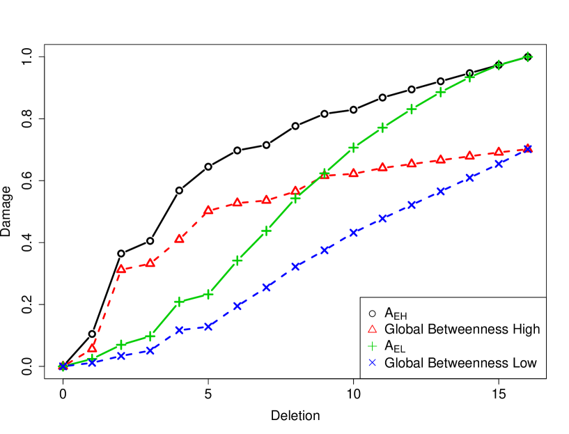
Figure 8: Damage to the discovered graph of path length 3 based on $A_{E,*}$  attack profiles. The “local” values are those that come from the discovered graph, while the global values are from the total graph. Damage inflicted on the discovered graph when using the high edge betweenness value and the resulting impact on the total graph are show in black and red respectively. In a similar manner, damage caused by choosing the low betweenness is shown in the green and blue lines respectively. The betweenness of each edge is recomputed after the removal of either the highest or lowest betweenness valued edge. The process is repeated again and again until all edges are removed.

C.4.2 Vertex selection

The attacker can compute the betweenness of any vertex in the subgraph that he has discovered (see Table 16) . Based on these computed betweenness values, the attacker can select either the highest or lowest valued vertex to remove. After the removal of this vertex, the betweenness values can be recomputed for the newly modified subgraph and the process repeated again and again until there are no vertices left in the discovered graph (the discovered graph is totally destroyed).

Figures 9 and 10 show the effects of repeatedly applying $A_{V,L}$  or $A_{V,L}$  profile to the discovered subgraph of path length 3. In each figure, the betweenness value of each vertex is written in the vertex. The vertex with the lowest (see Figure 9) or highest (see Figure 10) betweenness value is highlighted in yellow, prior to it being removed. After the removal of the vertex, the betweenness values of all the remaining vertices are computed and shown in the next subfigure, along with the next vertex that has been selected for removal. The four subfigures in Figures 9 and 10 show this process. When two or more vertices have the same betweenness value, the selection of which edge to remove it totally random.

Attack profile $A_{V,L}$  tends to attack the periphery of the subgraph. While attack profile $A_{V,H}$  tends to attack the core of the graph. While both selection choices will result in a fully disconnected graph with the same number of removals, selecting the highest valued vertex causes more damage quicker.

The betweenness computation, removal and damage computation process is shown in Table 19 and Figure 11. The global high line in Figure 11 goes flat after the fifth deletion while the global low line continues to increase. This behavior is explained by looking at Figures 12(a) and 12(b). By the fifth high deletion, the discovered and global graphs are disconnected and further local deletions do not affect the global graph. In Figure 12(a), the discovered and global graphs are still connected and local deletions will affect the global graph.

(a) First lowest has been identified

(b) Previous lowest has been removed, new lowest identified

(c) Previous lowest has been removed, new lowest identified

(d) Previous lowest has been removed, new lowest identified

Figure 9: The effects of an $A_{V,L}$  attack profile on the sample graph. Vertex 5 is the center vertex and is shown in red. The discovered graph, in pink is at a distance of 3 from the center vertex. Each vertex is labeled with the number of shortest paths that go use that vertex. The vertex with the lowest betweenness is drawn in yellow. Each time, the lowest valued vertex is removed from the discovered graph and all betweenness values for the discovered graph are recomputed. If there is more than one vertex with the same low value, one is selected at random for removal. Some of the vertices are unlabeled because the attacker has not “discovered” them.

(a) First highest has been identified

(b) Previous highest has been removed, new highest identified

(c) Previous highest has been removed, new highest identified

(d) Previous highest has been removed, new highest identified

Figure 10: The effects of an $A_{V,H}$  attack profile on the sample graph. Vertex 5 is the center vertex. The discovered graph is at a distance of 3 from the center vertex. The vertex with the highest betweenness is drawn in yellow. Each time, the highest valued vertex is removed from the discovered graph and all betweenness values for the discovered graph are recomputed. If there is more than one vertex with the same high value, one is selected at random for removal. Some of the vertices are unlabeled because the attacker has not “discovered” them.

Deletion	Local damage due to $A_{V,H}$	Global damage due to local damage by $A_{V,H}$	Local damage due to $A_{V,L}$	Global damage due to local damage by $A_{V,L}$
0	0.00	0.00	0.00	0.00
1	0.29	0.17	0.12	0.07
2	0.57	0.41	0.24	0.14
3	0.78	0.51	0.36	0.22
4	0.89	0.68	0.47	0.28
5	0.89	0.68	0.58	0.35
6	0.92	0.70	0.66	0.41
7	0.92	0.70	0.77	0.48
8	0.95	0.71	0.83	0.54
9	0.95	0.71	0.89	0.59
10	0.97	0.72	0.93	0.64
11	0.97	0.72	0.97	0.69
12	1.00	0.77	1.00	0.77

Table 19: Damage to the discovered subgraph of path length 3 based on $A_{V,*}$  attack profiles. The betweenness of each vertex is recomputed after the removal of either the highest or lowest betweenness valued vertex. The process is repeated again and again until all vertices are removed.

Figure 11: Damage to the discovered subgraph of path length 3 based on $A_{V,*}$  attack profiles. The “local” values are those that come from the discovered graph, while the global values are from the total graph. Damage inflicted on the discovered graph when using the high vertex betweenness value and the resulting impact on the total graph are show in black and red respectively. In a similar manner, damage caused by choosing the low betweenness is shown in the green and blue lines respectively. The betweenness of each vertex is recomputed after the removal of either the highest or lowest betweenness valued vertex. The process is repeated again and again until all vertices are removed. Damage to the global graph is flat from deletion 4 through 11, while the local damage increases due to the selection of the particular high valued vertices to remove. The low betweenness option does not show this type of behavior. The system of graphs for high and low selection is shown in Figure 12.

(a) Results of $A_{V,H}$ 

(b) Results of $A_{V,L}$ 

Figure 12: Markedly different graphs resulting from the differences in choosing $A_{V,H}$  or $A_{V,L}$  attack profiles. Both subfigures show the sample graph after 4 deletions based on $A_{V,H}$  or $A_{V,L}$  attack profiles. Continued deletions in the discovered graph (in pink) in the high betweenness case (see Figure 12(a)) , will have only marginal effect on the global graph (the union of pink and green). Deletions in the discovered graph in low betweenness case (see Figure 12(b)) will continue to affect the union of the pink and the green nodes because the two graphs (pink and green) are still connected. Some of the vertices are unlabeled because the attacker has not “discovered” them.

C.4.3 Degree selection

The attacker can compute the degreeness of any vertex in the subgraph that he has discovered (see Table 17) . Based on these values, the attacker can select either the highest or lowest valued vertex to remove. After the removal of this vertex, the degreeness values can be recomputed for the newly modified subgraph and the process repeated again and again until there are no vertices left in the discovered graph (the discovered graph is totally destroyed).

Figures 13 and 14 show the effects of repeatedly applying attack $A_{D,L}$  or $A_{D,L}$  profiles to the discovered subgraph of path length 3. In each figure, the degreeness value of each vertex is written in the vertex. The edge with the lowest (see Figure 13) or highest (see Figure 14) betweenness value is highlighted in yellow, prior to it being removed. After the removal of the vertex, the degreeness values of all the remaining vertices are computed shown in the next subfigure, along with the next vertex that has been selected for removal. The four subfigures in Figures 13 and 14 show this process. When two or more vertices have the same degreeness value, the selection of which edge to remove it totally random.

Attack profile $A_{D,L}$  tends to attack the periphery of the subgraph. While attack profile $A_{D,H}$  tends to attack the core of the graph. While both selection choices will result in a fully disconnected graph with the same number of removals, selecting the highest valued vertex causes more damage quicker.

The betweenness computation, removal and damage computation process is shown in Table 20 and Figure 15. The Global High line in Figure 15 goes flat after the fifth deletion while the Global Low line continues to increase. This behavior is explained by looking at Figures 16(a) and 16(b). Using a $A_{D,H}$  profile, the discovered and global graphs are disconnected and further local deletions do not affect the global graph. Using $A_{D,L}$  profile in Figure 16(b) results in the discovered and global graphs still being connected, so any deletions on the discovered graph affect the global graph. the fifth deletion the discovered and global graphs are

(a) First lowest has been identified

(b) Previous lowest has been removed, new lowest identified

(c) Previous lowest has been removed, new lowest identified

(d) Previous lowest has been removed, new lowest identified

Figure 13: The effects of an $A_{D,L}$  attack profile on the sample graph. Vertex 5 (marked in red) is the center vertex. The discovered graph is at a distance of 3 from the center vertex. The vertex with the lowest degree is marked in yellow. In the case where multiple vertices have the same degree value (see Figure 13(b)) , random choice is used to select one vertex as the next one to be removed. Removal of a vertex causes a reduction in the degree values of all of the removed vertex’s neighbors. This change in the degreeness of potentially many vertices requires that the relative order of the vertices be evaluated after each removal. Some of the vertices are unlabeled because the attacker has not “discovered” them.

(a) First highest has been identified

(b) Previous highest has been removed, new highest identified

(c) Previous highest has been removed, new highest identified

(d) Previous highest has been removed, new highest identified

Figure 14: The effects of on $A_{D,H}$  attack profile on the sample graph. Vertex 5 (marked in red) is the center vertex. The discovered graph is at a distance of 3 from the center vertex. The vertex with the highest degree is marked in yellow. In the case where multiple vertices have the same degree value (see Figure 14(c)) , random choice is used to select one vertex as the next one to be removed. Removal of a vertex causes a reduction in the degree values of all of the removed vertex’s neighbors. This change in the degreeness of potentially many vertices requires that the relative order of the vertices be evaluated after each removal. Some of the vertices are unlabeled because the attacker has not “discovered” them.

Deletion	Local damage due to $A_{D,H}$	Global damage due to local damage by $A_{D,H}$	Local damage due to $A_{D,L}$	Global damage due to local damage by $A_{D,L}$
0	0.00	0.00	0.00	0.00
1	0.27	0.16	0.12	0.07
2	0.61	0.37	0.24	0.14
3	0.78	0.51	0.36	0.22
4	0.88	0.62	0.47	0.28
5	0.95	0.74	0.58	0.35
6	0.97	0.75	0.66	0.41
7	1.00	0.76	0.77	0.48
8	1.00	0.76	0.83	0.54
9	1.00	0.76	0.89	0.59
10	1.00	0.76	0.93	0.64
11	1.00	0.76	0.97	0.69
12	1.00	0.76	1.00	0.77

Table 20: Damage to the discovered subgraph of path length 3 based on $A_{D,*}$  attack profiles. The degree of each vertex is computed after each deletion. A vertex’s degree value will change if one of it’s immediate neighbor vertices has been removed. The removal of a neighbor will reduce the degreeness of all its neighbors by one. This change in the degreeness of all neighboring vertices may affect the relative order of all vertices based on their respective degreeness. The process is repeated again and again until all edges are removed.

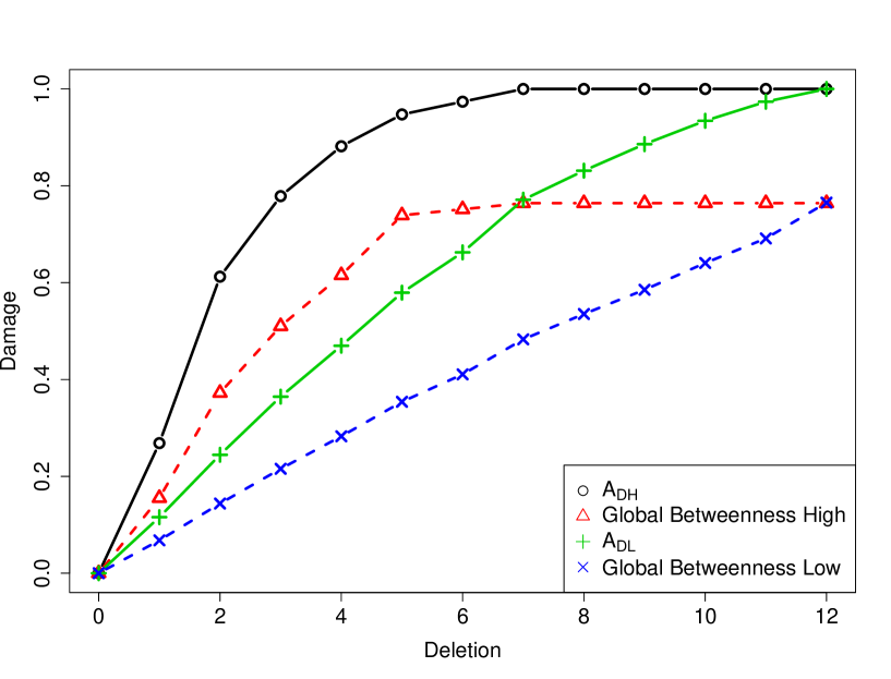
Figure 15: Damage to the discovered subgraph of path length 3 by based on $A_{D,*}$  attack profiles. The degree of each vertex is computed after each deletion. A vertex’s degree value will change if one of it’s immediate neighbor vertices have been removed. The removal of a neighbor will reduce the degreeness of all its neighbors by one. This change in the degreeness of all neighboring vertices may affect the relative order of all vertices based on their respective degreeness. The process is repeated again and again until all vertices are removed. The flat area on the Global High line is related to the discovered and global graphs becoming disconnected (see Figure 16) .

(a) High degree

(b) Low degree

Figure 16: The sample graph after removing the fifth discovered node using $A_{D,*}$  attack profiles. The undiscovered graph is drawn in green. The central vertex, where it remains is drawn in red (see Figure 16(b)) . The vertex that will be deleted next is drawn in yellow. While each graph shows the effects of five deletions, selecting the highest degreed node to delete results in a graph that is disconnected (see Figure 16(a)) . Focusing on the lowest degreed node results in damage to the periphery and a graph that is still connected (see Figure 16(b)) . Some of the vertices are unlabeled because the attacker has not “discovered” them.

C.5 Attack profile conclusions

All node based attacks ($A_{V,*}$ , $A_{D,*}$ ) will totally destroy the discovered graph. All edge based attacks $A_{E,*}$  will cause the discovered graph to be totally disconnected. The two attack philosophies differ in their efficacy and are summarized in Table 21.

If the attacker’s goal is to disconnect the sample graph by repeated use of the same attack profile, then the most effective profiles in order are: $A_{E,H}$ , $A_{V,H}$  and $A_{D,H}$ .

Attack Profile	Efficacy
$A_{D,H}$	Tends to attack the core of the graph
$A_{D,L}$	Tends to attack the periphery of the graph
$A_{E,H}$	Tends to attack the core of the graph
$A_{E,L}$	Tends to attack the periphery of the graph
$A_{V,H}$	Tends to attack the core of the graph
$A_{V,L}$	Tends to attack the periphery of the graph

Table 21: Efficacy of various attack profiles. In general, regardless of the attack profile utilized, attacking the highest valued component is the most destructive.

References

- [1] V. Ágoston, P. Csermely, and S. Pongor. Multiple weak hits confuse complex systems: a transcriptional regulatory network as an example. Physical Review E, 71(5):51909, 2005.
- [2] R. Albert, H. Jeong, and A.-L. Barabási. Error and Attack Tolerance of Complex Networks. Nature, 406(6794):378—382, July 2000.
- [3] A.-L. Barabási, R. Albert, and H. Jeong. Scale-Free Characteristics of Random Networks: The Topology of the World Wide Web. Physica A, 281(1):69—77, June 2000.
- [4] A. Beygelzimer, G. Grinstein, R. Linsker, and I. Rish. Improving Network Robustness by Edge Modification. Physica A: Statistical Mechanics and its Applications, 357(3-4):593—612, 2005.
- [5] B. Bollobás. Modern Graph Theory. 1998.
- [6] U. Brandes and T. Erlebach. Network Analysis: Methodological Foundations. 2005.
- [7] M. Brinkmeier and T. Schank. Network Statistics. Network Analysis, Lecture Notes in Computer Science, 3418:293—317, 2005.
- [8] R. Cohen, K. Erez, D. Ben-Avraham, and S. Havlin. Breakdown of the Internet Under Intentional Attack. Physical Review Letters, 86(16):3682—3685, 2001.
- [9] T. H. Cormen, C. E. Leiserson, and R. L. Rivest. Introduction to Algorithms. 1990. 1990.
- [10] R. Criado, J. Flores, B. Hernández-Bermejo, J. Pello, and M. Romance. Effective measurement of network vulnerability under random and intentional attacks. Journal of Mathematical Modelling and Algorithms, 4(3):307—316, 2005.
- [11] P. Crucitti, V. Latora, M. Marchiori, and A. Rapisarda. Error and attack tolerance of complex networks. Physica A: Statistical Mechanics and its Applications, 340(1-3):388—394, 2004.
- [12] A. Dekker. Simulating Network Robustness: Two Perspectives on Reality. In Proceedings of SimTecT 2004 Simulation Conference, pages 126—131, 2004.
- [13] K. I. Goh, E. Oh, H. Jeong, B. Kahng, and D. Kim. Classification of Scale-Free Networks. Proceedings National Academy of Sciences, 99(20):12583—12588, October 2002.
- [14] P. Holme, B. J. Kim, C. N. Yoon, and S. K. Han. Attack vulnerability of complex networks. Physical Review E, 65(5):56109, 2002.
- [15] G. W. Klau and R. Weiskircher. Robustness and Resilience. Network Analysis: Methodological Foundations, pages 417—437, 2005.
- [16] D. Koschützki, K. Lehmann, L. Peeters, S. Richter, D. Tenfelde-Podehl, and O. Zlotowski. Centrality Indices. Network Analysis, Lecture Notes in Computer Science, pages 16—61, 2005.
- [17] V. Latora and M. Marchiori. Vulnerability and protection of infrastructure networks. Physical Review E, 71(1):15103, 2005.
- [18] H. Lee and J. Kim. Attack Resiliency of Network Topologies. Parallel and Distributed Computing: Applications and Technologies, pages 638—641, 2004.
- [19] H. Lee, J. Kim, and W. L. Lee. Resiliency of Network Topologies under Path-Based Attacks. IEICE Transactions on Communications, 89(10):2878, 2006.
- [20] S. Netotea and S. Pongor. Evolution of robust and efficient system topologies. Cellular Immunology, 244(2):80—83, 2006.
- [21] D. Newth and J. Ash. Evolving cascading failure resilience in complex networks. In Proc. of 8th Asia Pacific Symposium on Intelligent and Evolutionary Systems. Citeseer, 2004.
- [22] A. Venuturumilli and A. Minai. Obtaining Robust Wireless Sensor Networks Through Self-organization of Heterogeneous Connectivity. In Proceedings of the 6th International Conference on Complex Systems. Citeseer, 2006.
- [23] X. F. Wang and G. Chen. Complex Networks: Small-World, Scale-Free and Beyond. IEEE circuits and systems magazine, 3(1):6—20, 2003.
- [24] D. J. Watts and S. H. Strogatz. Collective dynamics of ‘small world’ networks. Nature, 393:440—442, June 1998.
- [25] D. B. West. Introduction to Graph Theory. 2001.
- [26] Y. Yan-Ping, Z. Duan-Ming, T. Jin, P. Gui-Jun, and H. Min-Hua. Multiple Partial Attacks on Complex Networks. Chinese Physics Letters, 25:769, 2008.
- [27] E. Zio and G. Sansavini. Modeling failure cascades in network systems due to distributed random disturbances and targeted intentional attacks. Proceeding of the European Safety and Reliability Conference (ESREL 2008), 2008.