GRAVITATIONAL FRAGMENTATION OF EXPANDING SHELLS. II. THREE-DIMENSIONAL SIMULATIONS

Abstract

We investigate the gravitational fragmentation of expanding shells driven by HII regions using the three-dimensional Lagrangian simulation codes based on the Riemann solver, called Godunov smoothed particle hydrodynamics. The ambient gas is assumed to be uniform. In order to attain high resolution to resolve the geometrically thin dense shell, we calculate not the whole but a part of the shell. We find that perturbations begin to grow earlier than the prediction of the linear analysis under the thin-shell approximation. The wavenumber of the most unstable mode is larger than that in the thin-shell linear analysis. The development of the gravitational instability is accompanied by the significant deformation of the contact discontinuity. These results are consistent with a linear analysis presented by Iwasaki et al. that have taken into account the density profile across the thickness and approximate shock and contact discontinuity boundary conditions. We derive useful analytic formulae for the fragment scale and the epoch when the gravitational instability begins to grow.

1. Introduction

Massive stars strongly disturb the interstellar medium (ISM) via emission of ionizing photons, stellar winds, and supernova explosions. These processes produce overpressured hot bubbles that expand into ambient interstellar clouds. At the same time, a shock wave sweeps up the ambient clouds into a dense shell. The expanding shell strongly influences the dynamics of the ISM. Especially, it is often supposed to trigger the formation of stars through the gravitational fragmentation (Elmegreen & Lada, 1977). Hosokawa & Inutsuka (2005, 2006) investigated the dynamical expansion of the HII region, the photodissociation region, and the swept-up shell, solving the UV and far-UV radiative transfer and thermal and chemical processes in the one-dimensional (1D) hydrodynamics code. They showed that the shell becomes cold and dense enough for the gravitational instability (GI) to take place owing to the reformation of molecules destructed by far-UV photons. Numerous authors have discovered evidences for the star formation in shell-like molecular clouds around hot bubbles. Churchwell et al. (2006, 2007) have compiled a catalogue of $\sim 600$ shells from data in Spitzer-GLIMPSE survey. Recently, Deharveng et al. (2010) have investigated 102 samples identified as shells on the Spitzer-GLIMPSE images at 8.0$\mu$m. They found that 86% of the shells are associated with ionized gases, or HII regions. They obtained statistical properties of the triggered star formation, and suggested that more than a quarter of the shells may have triggered the formation of massive stars. This suggests that the trigger star formation process may be important in the massive star formation.

To understand the triggered star formation, it is important to investigate how and when the expanding shell fragments through the GI. Elmegreen (1994) and Whitworth et al. (1994) derived a simple dispersion relation taking into account the mass accretion and the dilution effect of perturbations owing to the expansion. They assumed the thin-shell approximation, and neglect the boundary effect of the contact discontinuity (CD). Recently, Iwasaki et al. (2011, hereafter Paper I) investigated stability of expanding shells taking into account asymmetric density profiles with imposing an approximate shock boundary condition on the leading surface and the CD boundary condition on the trailing surface. They found that the dispersion relation and eigen-function strongly depends on the boundary conditions and the degree of asymmetry of the density profile.

Although many authors have studied fragmentation of shells by using linear analysis, it is still uncertain how and when shells fragment. This is because the stability analysis of the evolving shell is difficult to perform without any approximations. Therefore, time-dependent multi-dimensional simulations are crucial to investigate it. To resolve propagating thin shells all the time, the Eulerian adaptive mesh refinement (AMR) technique in the mesh code or the smoothed particle hydrodynamics (SPH) have been used. However, since enormous meshes or SPH particles are required to resolve the thickness, researches based on numerical simulations are less advanced. Dale et al. (2007) investigated the gravitational fragmentation of the shell driven by the expansion of the HII region by using three-dimensional (3D) SPH taking into account the radiative transfer of ionizing photons. In their simulation, its thickness was not resolved sufficiently. Dale et al. (2009) have investigated fragmentation of shells with fixed mass that expand into a hot rarefied gas by using two different numerical schemes, the Eulerian AMR method (the flash code) and the SPH method. They considered shells confined by a constant pressure on both surfaces. In the more realistic situation where shells are confined by the CD and the shock front (SF), multi-dimensional simulations including the self-gravity have not been performed yet.

In this paper, we perform the 3D simulation to investigate the fragmentation process of expanding shells through GI. As numerical method, we adopt the 3D SPH method. In order to attain high resolution enough to resolve the thickness, we calculate not the whole but a part of the shell. The outline of the paper is as follows: in Section 2, we describe our model and simulations in detail. Brief review of Paper I is presented in Section 3. The results of our simulations are shown in Section 4. In Sections 5 and 6, we present discussions and summaries of our paper.

2. Simulations

2.1. Numerical Methods

We adopt the SPH method (e.g., Monaghan, 1992). Since SPH is Lagrangian particle method, it is one of the best method for problems where a wide low density region and geometrically thin shell coexist. Instead of additional viscosity to handle shocks, we use the “Godunov SPH” where the results of the Riemann problem are used to calculate the interaction between SPH particles (Inutsuka, 2002). The tree method (Barnes & Hut, 1986) is used to calculate self-gravitational force.

2.1.1 Treatment of Contact Discontinuity

In the standard SPH method (Monaghan, 1992), the $i$-th particle has the mass of $m_{i}$, and its density is given by

$$\rho_{i}=\sum_{k}m_{k}W({\bf x}_{i}-{\bf x}_{k},\bar{h}_{ik}),$$ (1)

where $W({\bf x},h)$ is kernel function and we use the Gaussian kernel, $h$ is the smoothing length, and $\bar{h}_{ik}$ is an average between $h_{i}$ and $h_{k}$. The equation of motion of the $i$-th particle is given by

$$\frac{\Delta{\bf v}_{i}}{\Delta t}=-\sum_{k}m_{k}\left(\frac{P_{i}}{\rho_{i}^{2}}+\frac{P_{k}}{\rho_{k}^{2}}\right)\frac{\partial}{\partial{\bf x}_{i}}W({\bf x}_{i}-{\bf x}_{k},\bar{h}_{ik}).$$ (2)

The standard SPH has a shortcoming when calculating the CD between a hot and a cold gas (Agertz et al., 2007). Agertz et al. (2007) reported that the artificial tension stabilizes the Kelvin-Helmholtz instability with a different densities in the standard SPH. In contrast, Cha et al. (2010) have shown that Godunov SPH can describe the Kelvin-Helmholtz instability reasonably well.

In addition, Tartakovsky & Meakin (2005) and Hu & Adams (2006) proposed a new method that treats the CD naturally in the context of a multi-phase fluid. They modified Equations (1) and (2) to treat the CD as follows:

$$\rho_{i}=m_{i}\sum_{k}W({\bf x}_{i}-{\bf x}_{k},\bar{h}_{ik}),$$ (3)

and

$$\frac{\Delta{\bf v}_{i}}{\Delta t} = -\frac{1}{m_{i}}\sum_{k}\left[P_{i}\left(\frac{m_{i}}{\rho_{i}}\right)^{2}+P_{k}\left(\frac{m_{k}}{\rho_{k}}\right)^{2}\right]$$ (4)

$$\hskip 85.35826pt\times\frac{\partial}{\partial{\bf x}_{i}}W({\bf x}_{i}-{\bf x}_{k}.\bar{h}_{ik}).$$

The term of $m_{i}/\rho_{i}$ represents the volume of $i$-th particle $\sim h_{i}^{3}$. Therefore, if we determine particle mass of hot and cold gases so that its smoothing length distributes smoothly across the CD, the terms inside the bracket in Equation (4) is smooth across the CD, leading to much better behavior at the CD. Their new method is very useful in problems where the position of the CD is known in advance as in our modeling. Equation (4) satisfies the relation of $m_{i}\Delta{\bf v}_{i}=-m_{k}\Delta{\bf v}_{k}$, suggesting that the momentum conservation is guaranteed. Furthermore, we apply the Godunov technique to Equation (4) as

$$\frac{\Delta{\bf v}_{i}}{\Delta t} = -\frac{1}{m_{i}}\sum_{k}P^{*}_{ik}\left[\left(\frac{m_{i}}{\rho_{i}}\right)^{2}+\left(\frac{m_{k}}{\rho_{k}}\right)^{2}\right]$$ (5)

$$\hskip 85.35826pt\times\frac{\partial}{\partial{\bf x}_{i}}W({\bf x}_{i}-{\bf x}_{k},\bar{h}_{ik}).$$

where $P^{*}_{ik}$ is the result of the Riemann problem between the $i$-th and the $k$-th particles (Inutsuka, 2002).

2.2. Models

Massive stars emit ultraviolet photons ($h\nu>13.6$ eV) and produce HII regions around them. Here, we consider a massive star that emits ionizing photons with the photon number luminosity $Q_{\mathrm{UV}}\>[\mathrm{s}^{-1}]$ into the ambient gas with the uniform density of $\rho_{\mathrm{E}}=mn_{\mathrm{E}}$, where $n_{\mathrm{E}}$ and $m$ are the number density and the mean mass of the ambient gas particle, respectively.

We construct as simple model as possible to concentrate on the physics of GI of expanding shells. Figure 1 illustrates the schematic picture of our model. In this paper, we do not calculate the radiative transfer of ionizing photons but introduce hot and cold gases that are assumed to evolve keeping their temperatures constant. The hot gas is occupied in $r<R_{\mathrm{CD}}$ (the dotted region), and the thin shell is in $R_{\mathrm{CD}}<r<R_{\mathrm{SF}}$, where $R_{\mathrm{CD}}$ and $R_{\mathrm{SF}}$ are positions of the CD and the SF, respectively. The pre-shock ambient cold gas in $r>R_{\mathrm{SF}}$ is assumed to be uniform. In our model, the inner boundary is set at $r=R_{\mathrm{b}}$ inside the hot bubble $(R_{\mathrm{b}}<R_{\mathrm{CD}})$. In the HII region, the detailed balance between the recombination and the ionization is approximately established all the time. Therefore, the interior pressure of the HII region is given by

$$P_{\mathrm{int}}=\rho_{\mathrm{E}}c_{\mathrm{II}}^{2}\left(\frac{R_{\mathrm{ST}}}{R_{\mathrm{CD}}}\right)^{3/2},$$ (6)

where $R_{\mathrm{ST}}$ is the Strömgren radius,

$$R_{\mathrm{ST}}=\left(\frac{3Q_{\mathrm{UV}}}{4\pi\alpha_{\mathrm{B}}n_{\mathrm{E}}^{2}}\right)^{1/3}.$$ (7)

We assume that the pressure of the HII region is spatially constant because of the high temperature. The hot gas at $r=R_{\mathrm{b}}$ is pushed by the interior pressure $P_{\mathrm{int}}$.

Figure 1.— Schematic picture of our model. The hot gas occupying the dotted region is embedded by the cold gas.

2.3. Calculation Domain

If we simulate the overall shell, the required number of SPH particles, $N_{\mathrm{tot}}$, is too large to calculate. Therefore, to save $N_{\mathrm{tot}}$, we calculate a part of the shell. The schematic picture of the calculation domain is shown in Figure 2, and is designated by $|\tan^{-1}(y/x)|\leq\theta_{\mathrm{b}}$ and $|\tan^{-1}(z/x)|\leq\theta_{\mathrm{b}}$. Since the solid angle subtended by the calculation domain from the center $O$ is given by

$$\Omega_{\mathrm{b}}\simeq 4\theta_{\mathrm{b}}^{2}\;\;\;\mathrm{for}\;\;\theta_{\mathrm{b}}\ll 1,$$ (8)

the total number of SPH particles can be reduced by a factor of $\Omega_{\mathrm{b}}/4\pi\sim\theta_{\mathrm{b}}^{2}/\pi$ compared with the calculation of the whole shell.

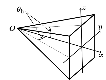
Figure 2.— Schematic picture of the calculation domain.

2.4. Simulation Units

In this paper, for convenience, the units of the time, length, and mass scales are taken to be

$$t_{0}=\sqrt{\frac{3\pi}{32G\rho_{\mathrm{E}}}}=1.6\;n_{\mathrm{E,3}}^{-1/2}\;\mathrm{Myr},$$ (9)

$$R_{0}=\left(\frac{7c_{\mathrm{II}}t_{0}}{\sqrt{12}}\right)^{4/7}R_{\mathrm{ST}}^{3/7}=5.9\;Q_{\mathrm{UV,49}}^{1/7}\>n_{\mathrm{E,3}}^{-4/7}\;\mathrm{pc},$$ (10)

and

$$M_{0}=\rho_{\mathrm{E}}R_{0}^{3}=5.0\times 10^{3}\;Q_{\mathrm{UV,49}}^{3/7}\>n_{\mathrm{E,3}}^{-5/7}\;M_{\odot},$$ (11)

respectively, where $Q_{\mathrm{UV,49}}=Q_{\mathrm{UV}}/10^{49}\>\mathrm{s}^{-1}$, and $n_{\mathrm{E,3}}=n_{\mathrm{E}}/10^{3}\>\mathrm{cm^{-3}}$. The dependence of the expansion law on the parameters $(Q_{\mathrm{UV}},\>n_{\mathrm{E}})$ are approximately eliminated by using the non-dimensional quantities normalized by $t_{0}$, $R_{0}$, and $M_{0}$ (see Figure 1 in Paper I).

2.5. Initial and Boundary Conditions

It is difficult to resolve very thin shell in early evolutionary phase even if we calculate the part of the shell (see Figure 2). Thus, we use a grid-based 1D hydrodynamical code to describe the early evolutionary phase of the HII region expansion, and we switch to 3D SPH at $t=0.4t_{0}$. As a grid-based numerical method, we use the 1D spherically symmetric Lagrangian Godunov method (van Leer, 1997). The innermost mesh at $R_{\mathrm{b}}$ is pushed by the interior pressure given by Equation (6). When the 1D simulation reaches $t/t_{0}=0.4$, the radial profiles of physical quantities are used as the initial condition of the 3D calculations. We smooth the distribution of the sound speed across the CD in the scale of the smoothing length. It is assumed that the temperature of the hot gas is 64 times as high as that of the cold gas. The specific value of the hot gas temperature does not change our conclusion as long as it is much larger than the temperature of the cold gas.

We calculate the expansions of HII regions around the 41$M_{\odot}$ (the high-mass (HM) model) and 19$M_{\odot}$ (the low-mass (LM) model) stars that are embedded by the uniform ambient gas of $n_{\mathrm{E}}=10^{3}$ cm^-3. Simulation parameters are listed in Table 1. The temperature of the cold gas $T_{\mathrm{c}}$ is assumed to be $10$ K. The opening angles of simulation domains are set to $\theta_{\mathrm{b}}=2\pi/26$ and $2\pi/14$ for the HM and the LM models, respectively, so that the calculation domains contain a single wavelength of the most unstable mode predicted from the thin-shell linear analysis by Elmegreen (1994). The mass of SPH particles are set so that the initial thickness is resolved by five SPH particles. Since the thickness increases with time, the relative resolution becomes better as the shell expands. In the later phase, the thickness is resolved by $\sim 15$ particles. The total number of SPH particles for the HM and the LM models are $4.00\times 10^{6}$ and $2.26\times 10^{6}$, respectively.

Corrugation-type perturbations are put into the shell at the initial state. We displace the SPH particles so that their densities do not change, or ${\bf\nabla}\cdot\Delta{\bf x}_{i}=0$, where $\Delta{\bf x}_{i}$ is the displacement of the $i$-th particle. The functional form of the displacement of the shell is assumed to be $\propto-\cos(l\phi)$, where $\phi=\tan^{-1}(y/x)$. Therefore, the shell has the negative displacement at $\phi=0$. The SPH particles are displaced keeping their velocity, the sound speed, and the mass fixed. We concentrate on the evolution of a single mode in each calculation. Dependence on $l$ is investigated by many runs.

The moving boundary condition at $r=R_{\mathrm{b}}(t)$ is realized by using “ghost particles” (Takeda et al., 1994). The time evolution of $R_{\mathrm{b}}(t)$ is obtained by the results of the 1D simulations. At the four surface areas ($y=\pm x\tan\theta_{\mathrm{b}}$, $z=\pm x\tan\theta_{\mathrm{b}}$) in the pyramid-shaped calculation domain (see Figure 2), the rotational periodic boundary condition is imposed.

Since the gravitational force is a long-range force, we have to take into account the particles in the whole solid angle. However, we only have information in the part of the solid angle as shown in Section 2.3. In this paper, the gravitational force is evaluated in the following method. Figure 3 shows the schematic picture of the gas sphere viewed from the $x$-direction for the case with $\theta_{\mathrm{b}}=2\pi/10$. The latitude and longitude lines are plotted at interval of $\theta_{\mathrm{b}}$. The region is surrounded by the thick solid lines represents the calculation domain (see Figure 2). We rotate the calculation domain $i\theta_{\mathrm{b}}$ degrees in the $\theta$-direction, where $i=-\pi/(2\theta_{\mathrm{b}}),\ldots,\pi/(2\theta_{\mathrm{b}})$. At each rotation step in the $\theta$-direction, we rotate the domain $k\theta_{\mathrm{b}}$ degrees in the $\phi$-direction, where $k=1,\ldots,2\pi/\theta_{\mathrm{b}}$. After that, the information in the whole solid angle can be obtained. However, for $i\neq 0$, the rotated domains in the $\phi$-direction have overlaps. This comes from the fact that the pyramid cannot fill 3D space. For example, the dashed regions in Figure 3 correspond to the rotated domains in the $\theta$-direction. We remove the overlapped SPH particles with $|\tan^{-1}(y/x)|>\theta_{\mathrm{b}}$ from the rotated domains. In the simulation, we rotate not SPH particles but the tree structure, and calculate the gravitational force from the rotated tree structures at each rotation step.

By this method, supposed particle distribution in the whole solid angular $4\pi$ is not cyclic completely. However, the effect of the approximation is negligible since $\theta_{\mathrm{b}}$ is very small in this paper. For $i=\pm 1$ (near the equatorial plane), the number of removed SPH particle is negligible compared with the total number. On the other hand, for large $|i|$ (near the poles), the fraction of removed SPH particles becomes large. However, since the rotated domain is very far from the calculation domain, the detail particle distribution is not important.

In this paper, we neglect the gravitational force outside the SF to prevent the ambient gas from collapsing toward the center. We find the radius $R_{\mathrm{grav}}$ of the most distant particle from the center that has density $\rho>\rho_{\mathrm{th}}$, where $\rho_{\mathrm{th}}$ is a threshold density (Bisbas et al., 2009). In our simulations, we adopt $\rho_{\mathrm{th}}=1.1\rho_{\mathrm{E}}$. Only SPH particles within $R_{\mathrm{grav}}$ are assumed to feel the gravitational force that is calculated above method. This means that there is the discontinuity in the gravitational force at the $R_{\mathrm{grav}}$. In the Appendix, we investigate the effect of the discontinuity, and confirm that it does not influence our results as long as $R_{\mathrm{grav}}$ is inside the shock transition layer. The main reason is that the pressure suddenly changes in the shock transition layer, suggesting that the pressure gradient is much larger than the jump in the gravitational force.

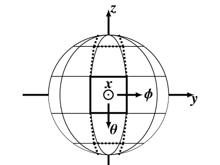
Figure 3.— Schematic picture viewed from the $x$-direction for the case with $\theta_{\mathrm{b}}=2\pi/10$. The latitude and longitude lines are plotted at interval of $\theta_{\mathrm{b}}$. The region is surrounded by the thick solid lines represents the calculation domain (see Figure 2). The dashed regions correspond to rotated domains in the $\theta$-direction.

Model	$M_{*}(M_{\odot})^{a}$	$R_{\mathrm{ST}}(\mathrm{pc})$	$R_{0}(\mathrm{pc})$	$T_{0}$(Myr)	$M_{0}(M_{\odot})$
High mass (HM)	41	0.56	5.5	1.6	$4.1\times 10^{3}$
Low mass (LM)	19	0.25	3.9	1.6	$1.46\times 10^{3}$

^a Mass of the star

Table 1Parameters of Our Models

2.6. Measures of Fluctuations

In order to evaluate growth of perturbations in the SPH calculations, we introduce indicators for fluctuations of density and the position of the CD. The solid angle $\Omega_{\mathrm{b}}$ is divided into $N_{\Omega}$ cells, and the direction of the $i$-th cell is defined by the unit vector ${\bf n}_{i}$ $(1\leq i\leq N_{\Omega})$. The radial profiles of the physical quantities along ${\bf n}_{i}$ are obtained from the SPH calculations. Here, we define the angle-dependent maximum density $\rho_{\mathrm{max}}({\bf n}_{i})$ along ${\bf n}_{i}$. The position of the CD along ${\bf n}_{i}$ is determined as the position where the temperature coincides with a critical value that is set to $\sqrt{2}T_{\mathrm{c}}$. The specific choice of the critical value is not important in our results. We average $\rho_{\mathrm{max}}({\bf n}_{i})$ and $R_{\mathrm{CD}}({\bf n}_{i})$ over all directions. The mean value of $Q=(\rho_{\mathrm{max}}$, $R_{\mathrm{CD}})$ is defined by

$$\langle Q\rangle=\frac{1}{N_{\Omega}}\sum_{i}Q({\bf n}_{i}).$$ (12)

As the indicators of the fluctuations, we evaluate the dispersions of these quantities

$$\Delta Q\equiv\sqrt{\frac{1}{N_{\Omega}}\sum_{i}\left\{Q({\bf n}_{i})-\langle Q\rangle\right\}^{2}}.$$ (13)

2.7. Unperturbed Evolution

As a test calculation, we present the evolution of the shell without initial perturbations in the HM model. Figure 4 shows the time evolution of $\langle R_{\mathrm{CD}}\rangle$ (Equation (12)) evaluated from the SPH simulation (the open circles). For comparison, we plot the result of the 1D simulation by the solid line. One can see that the SPH simulation can reproduce the results of the 1D calculation very well.

Figures 5 show snapshots of density (the upper panel) and pressure (the lower panel) profiles for $t/t_{0}=0.5$, 0.7, 1.0, and 1.26. The abscissae indicate the distance from the CD at each time. Only SPH particles in $|y|/R_{0}<0.05$ and $|z|/R_{0}<0.05$ are plotted by the dots. For comparison, the density profiles in the 1D simulation are superimposed by the thick gray lines in the upper panel. It is seen that the result of the SPH calculation agrees with that of the 1D simulation very well. Our 3D simulation clearly represents the structure and evolution of the shell although it is very thin.

Note that the pressure profiles in the lower panel of Figure 5 are smooth at the CD $(r-\langle R_{\mathrm{CD}}\rangle=0)$ thanks to the modified Godunov SPH shown in Section 2.1.1. In the standard SPH, a wiggle in pressure profile appears at the CD. In order to see whether the pressure profile is smooth even when perturbation is added, the density and pressure profiles for $t=1.0$ and $l=52$ are plotted in Figure 6. The detailed investigation of the results with perturbation is shown in Section 4. The abscissa is the distance from $\langle R_{\mathrm{CD}}\rangle$. We plot SPH particles in $\phi_{0}-\Delta\phi<\phi<\phi_{0}+\Delta\phi$ and $|z|/R_{0}<0.05$, where $\Delta\phi=0.001\theta_{\mathrm{b}}$. Figures 6(a) and (b) correspond to $\phi=0$ where $\delta\rho$ has the maximum value and $\phi_{0}=\theta_{\mathrm{b}}/2$ where $\delta\rho$ has the minimum value, respectively. One can clearly see that the pressure profile is smooth at the CD even with perturbation.

Figure 4.— Time evolution of $\langle R_{\mathrm{CD}}\rangle$. The open circles indicate the result of the SPH calculation. The solid line indicates the result of the 1D calculation.

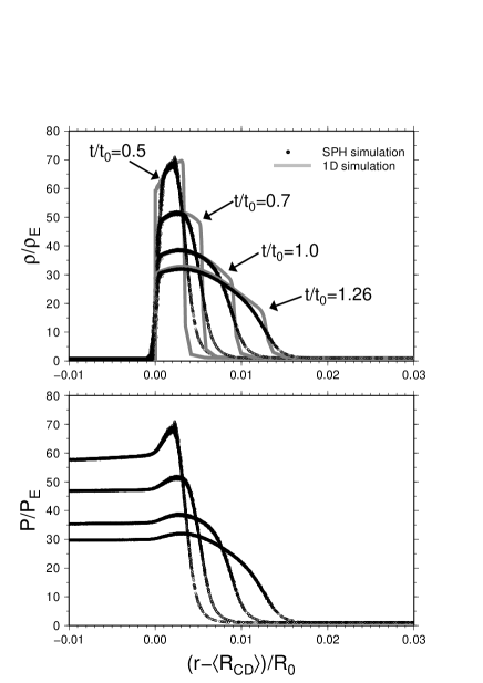
Figure 5.— Snapshots of density (the upper panel) and pressure (the lower panel) profiles for $t/t_{0}=0.5$, 0.7, 1.0, and 1.26. Only SPH particles in $|y|/R_{0}<0.05$ and $|z|/R_{0}<0.05$ are plotted by the dots. The abscissae are the distance from the CD. The thick gray lines in the upper panel indicate the results of the 1D simulation.

Figure 6.— Snapshots of the density and pressure profiles for $t/t_{0}=1.0$ and $l=52$. The abscissae are the distance from the average position of the CD. SPH particles in $\phi_{0}-\Delta\phi<\phi<\phi_{0}+\Delta\phi$ and $|z|/R_{0}<0.05$ are plotted, where $\phi_{0}=$(a)0, (b)$\theta_{\mathrm{b}}/2$, and $\Delta\phi=0.001\theta_{\mathrm{b}}$.

3. Prediction by Linear Analysis

Iwasaki et al. (2011) performed a linear analysis taking into account the thickness of the shell as in Figure 5 and imposing the approximate SF and the CD boundary conditions. They neglected evolutionary effect, i.e., expansion and mass accretion through the SF. At each instant of time, they solved eigen-value problem and obtained the growth rate $\Gamma(l,t)$ as a function of the time and the angular wavenumber, where $\Gamma$ is the imaginary part of $\omega(k,t)$ in Paper I. The angular wavenumber $l$ can be expressed as $2\pi R_{\mathrm{s}}/k$ by using the wavenumber $k$ in Paper I, where $R_{\mathrm{s}}$ is the shell radius.

3.1. Time Evolution and Scaling Law of Density Profile

The density profile of the decelerating shell is asymmetric with respect to the density peak. Iwasaki et al. (2011) developed a semi-analytic method for deriving the time evolution of the density profile by assuming that the shell reaches the hydrostatic equilibrium among the pressure gradient, the inertia force owing to the deceleration, and the radial gravitational force toward the center (Whitworth & Francis, 2002). Iwasaki et al. (2011) found that the time evolution of the density profile can be divided into three evolutionary phases, deceleration-dominated, intermediate, and self-gravity-dominated phases (see Figure 2 in Paper I). In the early phase (deceleration-dominated phase), the density peak is at the SF because the inertia force is larger than the gravitational force. As the shell expands, the inertia force decreases while the gravitational force increases. Thus, the density peak moves from the SF toward the CD as shown in Figure 5. In the intermediate phase, the density peak is closer to the SF than the CD. In the later phase (self-gravity-dominated phase), the density peak is closer to the CD than the SF.

It is also found that the density profiles for various sets of $(n_{\mathrm{E}},\;Q_{\mathrm{UV}})$ are characterized by a single parameter, that is the typical Mach number,

$${\cal M}_{0}=\frac{4}{7}\frac{R_{0}}{c_{\mathrm{s}}t_{0}}=7\;Q_{\mathrm{UV,49}}^{1/7}\>T_{\mathrm{c,10}}^{-1/2}\>n_{\mathrm{E,3}}^{-1/14},$$ (14)

where $T_{\mathrm{c,10}}=T_{\mathrm{c}}/10$ K.

They found the development of the GI is strongly influenced by two effects, asymmetry of the density profile and boundary conditions.

3.2. Asymmetry of the Density Profile

The asymmetry of the density profile strongly influences the GI, especially, in the self-gravity-dominated phase (for example, the shell at $t/t_{0}=1.26$ in Figure 5). In this later phase, the distance from the density peak to the SF is larger than $H_{0}$, where $H_{0}=c_{\mathrm{s}}/\sqrt{2\pi G\rho_{00}}$ is the scale height of the shell and $\rho_{00}$ is the peak density. On the other hand, the distance from the density peak to the CD is smaller than $H_{0}$. The gas tends to collect toward the density peak because the unperturbed gravitational potential has the minimum value there. The gas near the SF can collapse toward the density peak because the sound wave cannot travel from the density peak to the SF. This mode is “compressible mode”. On the other hand, the gas near the CD cannot collapse to the peak. However, the GI can proceed even there through the deformation of the CD that makes the gravitational potential deeper. This mode is “incompressible mode” (Elmegreen & Elmegreen, 1978; Lubow & Pringle, 1993). Therefore, the GI of the shell in the later phase has properties of compressible and incompressible modes.

Moreover, Iwasaki et al. (2011) found that the growth rate is enhanced compared with symmetric case through the combination of the GI and the Rayleigh-Taylor instability.

3.3. Boundary Conditions

Expanding shell is confined by the SF on the leading surface and by the CD on the trailing surface. Dispersion relations of Elmegreen (1994, E94) and Whitworth et al. (1994) are essentially based on the dispersion relation of the layer confined by the SF on both surfaces. The shock-confined layer is stabilized by the tangential flow generated by obliqueness of the SF compared with the layer confined by thermal pressure of hot gas. Therefore, the linear analysis in Paper I taking into account SF+CD boundary conditions gives larger growth rate compared with E94.

In summary, as described in Sections 3.2 and 3.3, Paper I predicts that the GI begins to grow earlier than the prediction from E94. The development of the GI in the later phase is accompanied by the significant deformation of the CD.

4. Results

4.1. The Case with High-mass Central Star

First, we present the results of the HM model with perturbations. We calculate four runs for the case with $l=26$, 52, 78, and 156. Figures 7(a), (b), (c), and (d) represent the time evolution of the perturbation amplitude for the wavenumber $l=26$, 52, 78, and 156, respectively. The thick solid and the thick dashed lines correspond to the density perturbation $\Delta\rho_{\mathrm{max}}/\langle\rho_{\mathrm{max}}\rangle$ and the deformation of the CD $30\times\Delta R_{\mathrm{CD}}$, respectively. In each panel, $\Delta\rho_{\mathrm{max}}/\langle\rho_{\mathrm{max}}\rangle$ and $\Delta R_{\mathrm{CD}}$ grow in the similar way. Perturbations with $l=52-78$ grow with the largest growth rate. For larger angular wavenumber $l=156$ and smaller angular wavenumber $l=26$, they grow more slowly. The prediction from E94 is also superimposed by the thin dashed line in each panel. It is found that in our 3D results, perturbations begin to grow earlier than the prediction of E94.

Let us compare the results of SPH simulations with the linear analysis in Paper I. However, Paper I neglected the evolutionary effects, i.e., expansion of the shell and the mass accretion through the SF. To include these effects approximately, we modify the instantaneous growth rate from $\Gamma$ to $\Gamma_{\mathrm{evo}}$ as follows:

$$\Gamma_{\mathrm{evo}}(l,t)\equiv-3\frac{V_{\mathrm{s}}(t)}{R_{\mathrm{s}}(t)}+\sqrt{\left(\frac{V_{\mathrm{s}}(t)}{R_{\mathrm{s}}(t)}\right)^{2}+\Gamma(l,t)^{2}},$$ (15)

where $V_{\mathrm{s}}$ is the velocity of the shell. This modification is inspired by E94. The time evolution of $R_{\mathrm{s}}(t)$ and $V_{\mathrm{s}}(t)$ is determined by the thin-shell model shown in Section 2 in Paper I. One can see that the terms of $V_{\mathrm{s}}/R_{\mathrm{s}}$ correspond to evolutionary effect of the shell that stabilizes the GI. The prediction based on Paper I is superimposed by the thin solid line in each panel of Figure 7. It is evaluated by $\exp\left[\int_{t}\Gamma_{\mathrm{evo}}(l,t^{\prime})\mathrm{d}t^{\prime}\right]$. From Figure 7, one can see that the linear analysis of Paper I describes the growth of perturbations very well.

Figure 8 shows the time sequence of cross sections through the $z=0$ plane for $l=52$. The color scale indicates density, and the arrows represent relative velocity to the fluid with the maximum density. The abscissa and the ordinate axes correspond to the azimuthal angle $\phi$, and the distance from the CD divided by $\langle R_{\mathrm{CD}}\rangle$, respectively. Figure 8(a) represents the initial condition where the shell around $\phi=0$ is displaced to the negative radial direction. Figure 8(b) shows that the tangential flow is generated by the obliqueness of the SF, and collects the gas around $\phi=0$. As a result, enhanced pressure pushes the SF outward in the radial direction (see Figure 8(c)). The gravitational potential around $\phi=0$ becomes deep, leading to gas accumulation (see Figure 8(d)). This mode of the GI is similar to the incompressible mode in the sense that the deformation develops at the boundary (Elmegreen & Elmegreen, 1978; Lubow & Pringle, 1993). In the later phase (Figure 8(e)), the CD highly deforms while the SF is almost flat. This is consistent with prediction of Paper I (see Section 3). Figure 8(e) is very similar to Figure 11 in Paper I that shows the eigenfunction in parameters of the HM model at $t/t_{0}=1.3$ for $l=52$.

Figure 9 is the same as Figure 8 but for larger wavenumber case, $l=156$. The initial state is shown in Figure 9(a). Because of large wavenumber, the tangential flow collects the gas more quickly in Figure 9(b) that is similar to Figure 8(c). In this moment, since the SF at $\phi=0$ deforms to the positive radial direction, the gas moves away from $\phi=0$ by the tangential flow. As a result, at $t/t_{0}=0.8$ (Figure 9(c)), the SF and the CD are almost flat while the velocity field exists inside the shell. The density distribution at $t/t_{0}=1.0$ (Figure 9(d)) has the opposite phase compared to the initial state. In this moment, the perturbation begins to grow but the growth rate is smaller than that for $l=52$. The CD deforms largely at the final state in both of Figures 8 and 9. In this sense, the behavior of the GI is similar to that for $l=52$.

Figure 7.— Time evolution of perturbations for the HM model. Each panel corresponds to $l=$ (a) 26, (b) 52, (c) 78, and (d) 156. The thick solid and the thick dashed lines represent the density perturbation $\Delta\rho_{\mathrm{max}}/\langle\rho_{\mathrm{max}}\rangle$ and the deformation of the CD $30\times\Delta R_{\mathrm{CD}}$, respectively. The thin solid lines correspond to the prediction from Paper I. The thin dashed lines correspond to the prediction based on Elmegreen (1994).

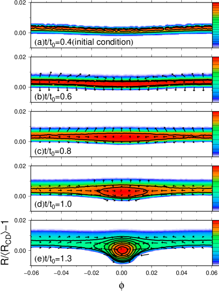
Figure 8.— Cross sections through the $z=0$ plane for $l=52$. Each panel shows the shell at $t/t_{0}=(a)0.4$, (b)0.6, (c)0.8, (d)1.0, and (d)1.3, respectively. The color scale represents the density, and arrows are velocities relative to the fluid at the density peak. The abscissa and the ordinate axes correspond to the azimuthal angle $\phi=\tan^{-1}(y/x)$, and $R/\langle R_{\mathrm{CD}}\rangle-1$, respectively.

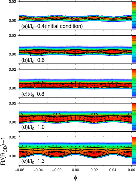
Figure 9.— Same as Figure 8 but for $l=156$.

4.2. The Case with Low Mass Central Star

Next, we present results of the LM model. Because the central star is less energetic, the Mach number of the expanding shell is smaller than that in the HM model, suggesting that the shell is geometrically thicker. Therefore, perturbations are expected to grow more slowly than the HM model. This feature is confirmed in Figure 10 that is similar to Figure 7. The most unstable mode is found in smaller wavenumber $l\sim 28$ and the growth rate is smaller than the HM model. We found that perturbations begin to grow earlier than the prediction of E94 also in this case. The linear analysis in Paper I describes the GI very well. Figure 11 shows the cross section through $z=0$ for $l=56$ at $t/t_{0}=1.5$. The significant deformation of the CD is seen as in the HM model.

Figure 10.— The same as Figure 7 but for the LM model. Each panel corresponds to $l=$(a)14, (b)28, (c)56, and (d)84.

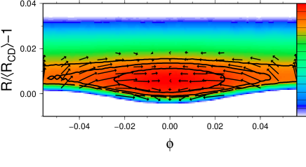
Figure 11.— Cross section through $z=0$ plane for $l=56$ at $t/t_{0}=1.5$ for the LM model. The color scale represents the density, and the arrows show velocities relative to the fluid at the density peak. The abscissa and ordinate axes are the same as Figure 8.

5. Discussion

5.1. Growth Rate of Gravitational Instability

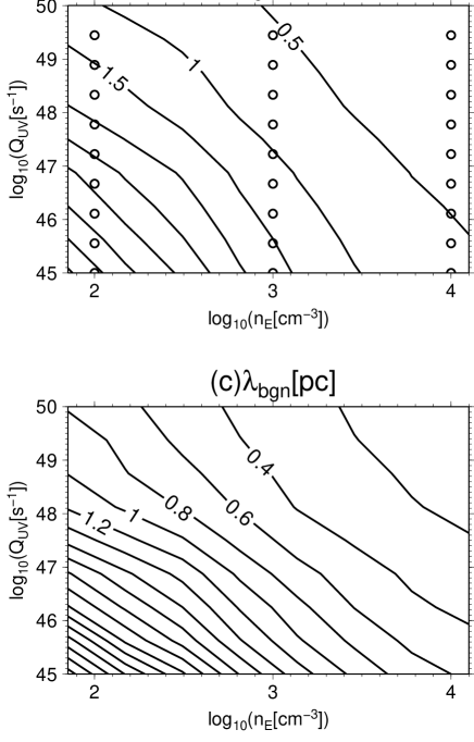
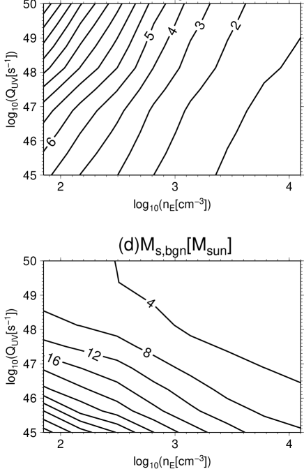
Figure 12.— Contour maps of (a)$t_{\mathrm{bgn}}$, (b)$R_{\mathrm{s,bgn}}$, (c)$\lambda_{\mathrm{bgn}}$, and (d)$M_{\mathrm{bgn}}$ in the $(\log_{10}n_{\mathrm{E}},\;\log_{10}Q_{\mathrm{UV}})$ plane. The open circles correspond to the parameters that are used in Figure 13.

We presented only two examples of the HM and the LM models in Section 4. In this section, we predict the GI in the shells with various parameters $(n_{\mathrm{E}},\;Q_{\mathrm{UV}},\;T_{\mathrm{c}})$ by using the results of the linear analysis presented in Paper I. As shown in Figures 7 and 10, it is found that the results of the SPH simulations are well described by the growth rate, $\Gamma_{\mathrm{evo}}$. Using this growth rate, one can predict the time $t_{\mathrm{bgn}}$ when the GI begins to grow by the condition $\Gamma_{\mathrm{evo}}(l_{\mathrm{bgn}},\;t_{\mathrm{bgn}})=0$, where $l_{\mathrm{bgn}}$ is the angular wavenumber of the most unstable mode at $t=t_{\mathrm{bgn}}$. This condition is rewritten as

$$\sqrt{8}\frac{V_{\mathrm{s}}}{R_{\mathrm{s}}}=\Gamma(l_{\mathrm{bgn}},\>t_{\mathrm{bgn}}),$$ (16)

where the left-hand side corresponds to the evolutionary rate owing to expansion and mass accretion, the right-hand side corresponds to the growth rate of the GI. At early phase, the evolutionary rate is larger than the growth rate of the GI, indicating that the shell is stable. As the shell expands, $V_{\mathrm{s}}/R_{\mathrm{s}}$ decreases while $\Gamma$ increases. Therefore, the GI begins to grow when the growth rate of the GI is larger than the evolutionary rate. The radius of the shell at $t=t_{\mathrm{bgn}}$ is defined by $R_{\mathrm{s,bgn}}$.

Figure 12(a), (b), (c), and (d) show contour maps of $t_{\mathrm{bgn}}$, $R_{\mathrm{s,bgn}}$, $\lambda_{\mathrm{max}}\equiv 2\pi R_{\mathrm{s,bgn}}/l_{\mathrm{bgn}}$, and $M_{\mathrm{bgn}}\equiv\Sigma(t=t_{\mathrm{bgn}})\pi(\lambda_{\mathrm{bgn}}/2)^{2}$ in the $(n_{\mathrm{E}},\;Q_{\mathrm{UV}})$ plane derived by using the linear analysis, respectively. Here, $T_{\mathrm{c}}$ is assumed to be 10 K. From Figures 12, one can see that the $t_{\mathrm{bgn}}$, $R_{\mathrm{s,bgn}}$, $\lambda_{\mathrm{bgn}}$, and $M_{\mathrm{bgn}}$ decrease with increasing $n_{\mathrm{E}}$. This can be understood by scaling of the typical number density of the shell, $n_{\mathrm{sh}}=n_{\mathrm{E}}{\cal M}_{0}^{2}$ that corresponds to the shocked gas density. From Equation (14), we have $n_{\mathrm{sh}}\propto n_{\mathrm{E}}^{6/7}$. Therefore, for larger $n_{\mathrm{E}}$, the shell becomes denser and unstable earlier (Figure 12(a)), and the most unstable scale is smaller (Figures 12(c) and (d)). Next, let us see the dependence of $t_{\mathrm{bgn}}$, $R_{\mathrm{s,bgn}}$, $\lambda_{\mathrm{bgn}}$, and $M_{\mathrm{bgn}}$ on $Q_{\mathrm{UV}}$. Since the central star is more energetic for larger $Q_{\mathrm{UV}}$, the Mach number of the expanding shell $\left({\cal M}_{0}\propto Q_{\mathrm{UV}}^{1/7}\right)$ is larger, indicating that the shell is denser and is more unstable. Therefore, $t_{\mathrm{bgn}}$, $\lambda_{\mathrm{bgn}}$, and $M_{\mathrm{bgn}}$ decreases with increasing $Q_{\mathrm{UV}}$. On the other hand, $R_{\mathrm{s,bgn}}$ increases with $Q_{\mathrm{UV}}$ because the expansion velocity increases with $Q_{\mathrm{UV}}$.

Figure 13.— Dependence of (a)$t_{\mathrm{bgn}}/t_{0}$, (b)$R_{\mathrm{s,bgn}}/R_{0}$, and (c)$l_{\mathrm{max}}$ on the typical Mach number ${\cal M}_{0}$. The open circles correspond to the results of linear analysis. The solid lines indicate the analytic formulae.

From Figures 12, since the contour lines are almost straight in the plane $(\log_{10}n_{\mathrm{E}},\>\log_{10}Q_{\mathrm{UV}})$, quantities are expected to have power-law dependence on $Q_{\mathrm{UV}}$ and $n_{\mathrm{E}}$, or equivalently on ${\cal M}_{0}$. In Figure 13, we plot $t_{\mathrm{bgn}}/t_{0}$, $R_{\mathrm{s,bgn}}/R_{0}$, and $l_{\mathrm{bgn}}$ as a function of ${\cal M}_{0}$ for various parameters that correspond to the open circles in Figure 12. The open circles correspond to the results of the linear analysis. From Figures 13, one can see that the results of the linear analysis are well described by the analytic formulae, $t_{\mathrm{bgn}}/t_{0}=1.62{\cal M}_{0}^{-0.75}$, $R_{\mathrm{s,bgn}}/R_{0}=1.2{\cal M}_{0}^{-0.375}$, and $l_{\mathrm{bgn}}=3.2{\cal M}_{0}^{1.5}$ that are plotted by the solid lines. Using Equation (14), the analytic formulae are rewritten as

$$t_{\mathrm{bgn}}=0.6\>Q_{\mathrm{UV,49}}^{-0.11}\>T_{\mathrm{c,10}}^{0.375}\>n_{\mathrm{E,3}}^{-0.45}\;\mathrm{Myr},$$ (17)

$$R_{\mathrm{s,bgn}}=3.4\>Q_{\mathrm{UV,49}}^{0.09}\>T_{\mathrm{c,10}}^{0.19}\>n_{\mathrm{E,3}}^{-0.54}\;\mathrm{pc},$$ (18)

and

$$l_{\mathrm{bgn}}=54\;Q_{\mathrm{UV,49}}^{0.21}\>T_{\mathrm{c,10}}^{-0.75}\>n_{\mathrm{E,3}}^{-0.11}.$$ (19)

The wavelength $\lambda_{\mathrm{bgn}}$ and the mass $M_{\mathrm{bgn}}$ that correspond to $l_{\mathrm{bgn}}$ are given by

$$\lambda_{\mathrm{bgn}}=0.4\;Q_{\mathrm{UV,49}}^{-0.125}\>T_{\mathrm{c,10}}^{0.94}\>n_{\mathrm{E,3}}^{-0.44}\;\mathrm{pc},$$ (20)

and

$$M_{\mathrm{bgn}}=3.5\;Q_{\mathrm{UV,49}}^{-0.16}\>T_{\mathrm{c,10}}^{2.06}\>n_{\mathrm{E,3}}^{-0.42}\;\mathrm{M_{\odot}},$$ (21)

Whitworth et al. (1994, W94) also derived similar formulae by using the thin-shell linear analysis similar to E94. The dependence of Equations (17)-(21) on parameters $Q_{\mathrm{UV}}$, $T_{\mathrm{c}}$, and $n_{\mathrm{E}}$ shows close agreement with that in W94 although the numerical factors are different. Our results show that the GI begins to grow earlier and as a result, the fragment mass is smaller than their results. In detail, $t_{\mathrm{bgn}}$, $R_{\mathrm{bgn}}$, and $\lambda_{\mathrm{bgn}}$ are roughly half of those in W94, and $M_{\mathrm{bgn}}$ is roughly 1/8 of that in W94. This is because the stabilization effect of the SF does not work on the trailing surface that is the CD as shown in Paper I. As pointed out in W94, the properties of fragments are insensitive to $Q_{\mathrm{UV}}$, and mainly depend on $n_{\mathrm{E}}$ and $T_{\mathrm{c}}$. Indeed, in Equations (20) and (21), the dependence of $\lambda_{\mathrm{bgn}}$ and $M_{\mathrm{bgn}}$ on $n_{\mathrm{E}}$ are close to the Jeans length and the Jeans mass of the shell $(\lambda_{\mathrm{J}},\;M_{\mathrm{J}})\propto n_{\mathrm{sh}}^{-1/2}\propto n_{\mathrm{E}}^{-3/7}$.

5.2. Comparison with Previous Studies

Elmegreen (1989) investigated the GI in a decelerating shocked layer. He numerically integrated perturbation equations with respect to time by taking into account time evolution of the layer and by averaging physical quantities over the thickness. He has taken into account SF and CD boundary conditions on the SF and CD, respectively. He called the boundary effect on the CD “pinching force”. In his linear analysis, the destabilizing effect of the pinching force does not work efficiently. One reason is that he used Equation (3) in Paper I as the pressure of the HII region although the geometry is plane-parallel. Therefore, the pressure at the CD is underestimated, leading to underestimate the pinching force of the CD. The other reason is the geometry of the gravitational potential. Asymmetry of density profile of spherical shell is qualitatively different from that of plane-parallel layer. In the plane-parallel geometry, the static symmetric layer peaks at the mid-plane. If the layer decelerates, the density peak is always closer to the SF than the CD. Therefore, the tangential flow behind SF erodes the density perturbation more efficiently. On the other hand, for the case with shells, the peaks can be closer to the CD than the SF (see Section 3.1). From these reasons, he derived lower growth rates than our results.

Dale et al. (2009) simulated the gravitational fragmentation of expanding shells confined by temporary constant thermal pressure of hot rarefied gases on both sides. In their calculation, the motion of the shell is determined so that the pressure at the leading surface is the same as that at the trailing surface. Therefore, the density peak is always around the mid-plane of the shell, and the density profile is almost symmetric. In their calculation, the column density decreases with time because the shell expands keeping the mass fixed. Therefore, the pressures at the boundaries approach to the peak pressure. They found that the confining pressure accelerates fragmentation in the later phase, and describe this effect as “pressure-assisted” gravitational fragmentation. This mode is the same as the incompressible mode. Recently, taking into account the effect of the thickness of the shell approximately, Wünsch et al. (2010) established a semi-analytic linear analysis that explains results of their SPH simulations. Different from them, in Paper I, we have taken into account the effect of SF+CD boundary condition approximately.

5.3. Other Instabilities

We discuss other potentially important effects that are not analyzed in this paper.

5.3.1 Vishniac Instability

Vishniac (1983) found a hydrodynamical overstability on decelerating shells confined by the SF on the leading surface and by the CD on the trailing surface by using thin-shell linear analysis. However, the Vishniac instability (VI) did not appear to occur in our simulations. This can be explained by the stabilizing effect by expansion. Vishniac & Ryu (1989) obtained an analytic dispersion relation of the VI of the expanding shell without self-gravity by taking into account the thickness approximately. In Section 6 in Paper I, they discussed the VI by applying the analytic dispersion relation to the shell driven by the HII region. They found that the VI is expected not to be important in the later phase ($t/t_{0}>0.5$) since its growth rate is comparable to the expansion rate of the shell radius. Therefore, the VI was not found in our simulation. However, they also found that before the beginning time of our simulations ($t/t_{0}<0.4$), the VI is expected to grow rapidly since the Mach number is large (see Figure 13 in Paper I). The perturbations quickly reach the nonlinear regime and saturate as a subsonic transverse flow (Mac Low & Norman, 1993). As a results, a small scale subsonic turbulence whose angular wavelength of $l=10^{2}\sim 10^{3}$ is expected to be induced. The consequence of VI may correspond to the increase of the initial perturbations in our 3D simulation.

5.3.2 Thermal Instability

In this paper, we assume that the fluid evolves keeping its temperature fixed. However, in real interstellar medium (ISM), shock-heated gas cools via radiative cooling. It is well known that the cooling ISM is often thermally unstable. In such a case, during the cooling condensation, the layer is expected to fragment into dense clouds with various scales (Iwasaki & Tsuribe, 2009). Koyama & Inutsuka (2002) investigated the propagation of a shock wave into the warm neutral medium. They found that cold cloudlets move with supersonic velocity dispersion in surrounding warm gas in the postshock region. The velocity dispersion is larger than the sound speed of cloudlets while it is smaller than the sound speed of surrounding warm gas. Since the shocked molecular cloud is also thermally unstable, the thermal instability drives supersonic turbulence inside the shell, and cold molecular cloudlets move with the supersonic velocity dispersion. This situation is quite different from the isothermal gas that has been considered in this paper. The supersonic turbulence is expected to be important in contrast to the subsonic turbulence driven by the VI, and considerably modify the evolution. The mass of the cold molecular cloudlets increases with time through the accretion of surrounding gas and the coalescence between cloudlets. The supersonic turbulence may provide effective turbulent pressure, while coalescence of cold cloudlets may decrease turbulent pressure. We will address the effect of the thermal instability on the GI of the expanding shells in our next work.

5.4. Ionization Front

In the paper, we did not solve the radiative transfer equation of the ionizing photons. Instead, we assumed that the trailing surface is the CD instead of the ionization front (IF). There are two effects of the ionization on the GI. One is that a fraction of the shell becomes ionized gas as HII region expands. Therefore, our simulations overestimate the column density of the shell. The swept-up mass by the SF is given by

$$M_{\mathrm{sw}}=\frac{4\pi}{3}\rho_{\mathrm{E}}R_{\mathrm{s}}^{3}.$$ (22)

On the other hand, the ionized mass is given by

$$M_{\mathrm{ion}}=\frac{4\pi}{3}\rho_{\mathrm{i}}R_{\mathrm{s}}^{3},$$ (23)

where $\rho_{\mathrm{i}}$ is the density of the ionized gas, and we neglect the difference between radii of the IF and SF. The real shell mass is given by $M_{\mathrm{sw}}-M_{\mathrm{ion}}$. Inside the HII region, the balance between the ionization and the recombination is approximately established. Therefore, the density of the HII region becomes

$$\rho_{i}=\left(\frac{3m^{2}Q_{\mathrm{UV}}}{4\pi\alpha_{\mathrm{B}}R_{\mathrm{s}}^{3}}\right)^{1/2}=\rho_{\mathrm{E}}\left(\frac{R_{\mathrm{ST}}}{R_{\mathrm{s}}}\right)^{3/2},$$ (24)

where $m$ is the mean weight of the gas particles and we use Equation (7). Therefore, from Equations (22)-(24), the ratio of $M_{\mathrm{ion}}$ to $M_{\mathrm{sw}}$ is

$${\cal R}\equiv\frac{M_{\mathrm{ion}}}{M_{\mathrm{sw}}}=\left(\frac{R_{\mathrm{ST}}}{R_{\mathrm{s}}}\right)^{3/2}.$$ (25)

If ${\cal R}\ll 1$, the effect of the ionization is negligible. In Figure 1 in Paper I (also see Figure 4), the Strömgren radius is as large as $0.1R_{0}$ in various parameters $(Q_{\mathrm{UV}},\;n_{\mathrm{E}})$. At the beginning time of our simulations, $t=0.4t_{0}$ $(R_{\mathrm{s}}\sim 0.6R_{0})$, ${\cal R}\sim(0.1/0.6)^{3/2}=0.07$. As the shell expands, ${\cal R}$ decreases. At $t=t_{0}$, ${\cal R}\sim(0.1/10)^{3/2}\sim 0.03$. Therefore, the contribution of the ionization is limited to only several percent.

The other is that the IF induces an instability on the shell. The D-type IF is analogous to a combustion front that is unstable to corrugational deformations (Landau & Lifshitz, 1987). Vandervoort (1962) found that the D-type IF is unstable. In this instability, the most unstable scale is comparable to the thickness of the IF. Moreover, Garcia-Segura & Franco (1995) showed that the VI is strongly modified by the IF. The shell rapidly fragments and finger-like structures are generated in their two-dimensional simulations. Note, however, that they assumed the power-law density distribution $\propto r^{-w}$ of the ambient gas with the uniform density core in the center with $0.2$ pc, where parameter $w$ is set to 2. The expansion of the IF depends on the power-law index $w$ in the 1D model. If $w>1.5$, even if the SF is emerged in front of the IF in the uniform density core, the IF quickly gets ahead of the SF, and eventually the whole of the shell and the ambient gas are ionized. Moreover, Hosokawa (2007) investigated the expansion of the IF and the dissociation front, and showed that the star formation is expected to be suppressed when $w>1$. This is because the column density decreases as the shell expands and the FUV photon easily escapes in front of the shock. Therefore, model by Garcia-Segura & Franco (1995) corresponds to the case where the triggered star formation is not simply expected. We need to investigate the expansion of the IF for the case with the shallower density profile $w<1$ in detail using the radiative multi-dimensional simulations taking into account the self-gravity. Moreover, Williams (1999) discovered shadowing instability in the R-type IF before emerging of the SF. This instability may also disturb the shell in the very early phase of evolution.

5.5. Magnetic Field

It is well known that the magnetic field is important in the dynamics of the ISM although it is neglected in this paper. Nagai et al. (1998) investigated the GI of a pressure-confined isothermal layer threaded by uniform magnetic field by using linear analysis. They found that the magnetic field cannot stabilize the GI. Moreover, they found the layer fragment in filamentary clouds whose longitudinal axis is parallel or perpendicular to the magnetic field depending on the thickness of the layer. However, their analysis is restricted to the static magnetized layer. It is important to investigate stability of magnetized shocked layer or shell in dynamical modeling.

6. Summary

In this paper, we have investigated the GI of the expanding shell using 3D numerical simulation with high resolution. We summarize our results as follows:

1. The GI begins to grow earlier than the prediction from the linear analysis based on the thin-shell approximation (Elmegreen, 1994; Whitworth et al., 1994). During the development of the GI, the contact discontinuity highly deforms while the shock front remains almost flat. These all features are consistent with the prediction from Iwasaki et al. (2011).

2. The GI is expected to begin to grow at an epoch when the growth rate of the GI becomes larger than the evolutionary rate owing to the expansion and the mass accretion (see Equation (16)) Using the results of the linear analysis, we have derived useful approximate analytic formulae (Equations (17)-(21)) for the fragment scale and the epoch when the GI starts.

This paper and Paper I revisit the fragmentation of the expanding shells by using both the 3D simulation and the linear analysis. Since the gas is subject to heating owing to far-UV photon, the gas temperature is larger than 10 K (Hosokawa & Inutsuka, 2005, 2006). When $T_{\mathrm{c}}=30$ K ($50$ K), the GI with mass scale of $M_{\mathrm{bgn}}\sim 34\>M_{\odot}\>$ ($96$ $M_{\odot}$) begins to grow at $t_{\mathrm{bgn}}\sim 0.9$ Myr (1.1 Myr) ($Q_{\mathrm{UV}}=10^{49}$ s^-1, $n_{\mathrm{E}}=10^{3}$ cm^-3) from Equations (17) and (21). The fragment mass is expected to be larger than $M_{\mathrm{bgn}}$ because it increases through the gas accretion. Moreover, perturbations with larger scale than the most unstable mode is also unstable. Therefore, the larger scale perturbations gradually grows, and small scale fragments may coalesce into larger one, and the total number of fragments may decrease. The predicted masses are roughly comparable to (or are slightly smaller than) observational masses of dense cores (dozens $\sim$ hundreds M_⊙) (e.g., Deharveng et al., 2003; Zavagno et al., 2006) although our model is based on very idealized situation, such as uniform ambient gas and isothermal equation of state.

Appendix A Effect of Discontinuity in Gravitational Force

In this paper, the gravitational force is neglected outside $R_{\mathrm{grav}}$ (see Section 2.5). We investigate how the sudden change in the gravitational force at $R_{\mathrm{grav}}$ influences our results. To see this, we focus on the time evolution of the displacement of the SF $\Delta R_{\mathrm{SF}}$ whose definition is the same as $\Delta R_{\mathrm{CD}}$ (see Section 2.6). When $\Delta R_{\mathrm{SF}}$ is evaluated, the position of the SF along ${\bf n}_{i}$ is determined as the density coincides with $1.1\rho_{\mathrm{E}}$. Figure 14(a) shows that the time evolution of $\Delta R_{\mathrm{SF}}$ for $l=52$ in the HM model. The solid line and the open circles correspond to $\rho_{\mathrm{th}}=1.1\rho_{\mathrm{E}}$ and $2\rho_{\mathrm{E}}$, respectively. One can see that they agree very well. Therefore, our results are insensitive to the position of the discontinuity of the gravitational force. This is because the pressure gradient is much larger than the gravitational force at the shock transition layer. This is clearly seen in Figure 14(b) that shows the pressure gradient, the gravitational force and the density at $t=t_{0}$ for $l=52$ in the simulation unit. The SPH particles around $\phi=0$ is plotted. The threshold density is set to $1.1\rho_{\mathrm{E}}$. One can see that the gravitational force has the jump around $(r-\langle R_{\mathrm{C}}\rangle)/R_{0}\sim 0.013$ that corresponds to $R_{\mathrm{grav}}$ in Figure 14(b). From Figure 14(b), the discontinuity in the gravitational force is much smaller than the pressure gradient because the pressure suddenly changes at the shock transition layer.

Therefore, it is concluded that the existence of the discontinuity in the gravitational force is not important as long as the discontinuity is inside the shock transition layer.

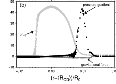
Figure 14.— a) Time evolution of the displacement of the SF. The solid line and the open circles correspond to $\rho_{\mathrm{th}}=1.1\rho_{\mathrm{E}}$ and $2\rho_{\mathrm{E}}$, respectively. b) Snapshots of the pressure gradient (the light gray circles), and the gravitational force (the dark gray circles) along the $r$-direction in the simulation unit. The density distribution is superimposed by the filled circles. The abscissae are the distance from the CD.

References

- Agertz et al. (2007) Agertz, O. et al. 2007, MNRAS, 370, 963
- Barnes & Hut (1986) Barnes, J. & Hut, P. 1986, Nature, 324, 446
- Bisbas et al. (2009) Bisbas, T. G., Wünsch, R., Whitworth, A. P., & Hubber, D. A. 2009, MNRAS, 497, 649
- Cha et al. (2010) Cha, S., Inutsuka, S., & Sergei, N. 2010, MNRAS, 403, 1165
- Churchwell et al. (2006) Churchwell, E. et al., 2006, ApJ, 649, 759
- Churchwell et al. (2007) Churchwell, E. et al., 2007, ApJ, 670, 428
- Dale et al. (2007) Dale, J. E., Bonnell, I. A. & Whitworth, A. P. 2007, MNRAS, 375, 1291
- Dale et al. (2009) Dale, J. E., Wünsch, R., Whitworth, A. P., & Palouš, J. 2009, MNRAS, 398, 1537
- Deharveng et al. (2003) Deharveng, L., Lefloch, B., Zavagno, A., Caplan, J., Whitworth, A. P., Nadeau, D., & Martín, S. 2003, A&A, 408, L25
- Deharveng et al. (2010) Deharveng, L., et al. 2010, A&A, 523, A6
- Elmegreen & Elmegreen (1978) Elmegreen, B. G., & Elmegreen, D. M. 1978, ApJ, 220, 1051
- Elmegreen (1994) Elmegreen, B. G. 1994, ApJ, 427, 384
- Elmegreen (1989) Elmegreen, B. G. 1989, ApJ, 340, 786
- Elmegreen & Lada (1977) Elmegreen, B. G., & Lada, C. J. 1977, ApJ, 214, 725
- Garcia-Segura & Franco (1995) Garcia-Segura, G., & Franco, J. 1995, ApJ, 469, 171
- Hosokawa & Inutsuka (2005) Hosokawa, T., & Inutsuka, S. 2005, ApJ, 623, 917
- Hosokawa & Inutsuka (2006) Hosokawa, T., & Inutsuka, S. 2006, ApJ, 646, 240
- Hosokawa (2007) Hosokawa, T. 2007, å, 463, 187
- Hu & Adams (2006) Hu, X. Y., & Adams, N. A. 2006, J. Comp. Phys., 213, 844
- Inutsuka (2002) Inutsuka, S. 2002, J. Comp. Phys., 179, 238
- Iwasaki et al. (2011) Iwasaki, K., Inutsuka, S., & Tsuribe, T. 2011, ApJ, in press
- Iwasaki & Tsuribe (2009) Iwasaki, K. & Tsuribe, T. 2009, A&A, 508, 725
- Koyama & Inutsuka (2002) Koyama, H. & Inutsuka, S. 2002, ApJ, 564, 97
- Landau & Lifshitz (1987) Landau, L. D., & Lifshitz, E. M. 1987, Fluid Mechanics (2nd rev. ed.; New York: Pergamon)
- Lubow & Pringle (1993) Lubow, S. H., & Pringle, J. E. 1993, MNRAS, 263, 701
- Mac Low & Norman (1993) Mac Low, M. & Norman, M. L. 1993, ApJ, 407, 207
- Monaghan (1992) Monaghan, J. J. 1992, ARA&A, 345, 561
- Nagai et al. (1998) Nagai, T, Inutsuka, S., & Miyama, S. M. 1998, ApJ, 506, 306
- Tartakovsky & Meakin (2005) Tartakovsky, A. M. & Meakin, P. 2005, J. Comp. Phys., 207, 610
- Takeda et al. (1994) Takeda, H., Miyama, S. M., & Sekiya, M. 1994, Prog. Theor. Phys., 92, 939
- Vandervoort (1962) Vandervoort, P. O. 1962, ApJ, 135, 212
- van Leer (1997) van Leer, B. 1997, J. Comp. Phys., 135, 229
- Vishniac (1983) Vishniac, E. T. 1983, ApJ, 274, 152
- Vishniac & Ryu (1989) Vishniac, E. T. & Ryu, D, 1989, ApJ, 337, 917
- Whitworth et al. (1994) Whitworth, A. P., Bhattal, A. S., Chapman, S. J., Disney, M. J., & Turner, J. A. 1994, MNRAS, 268, 291
- Whitworth & Francis (2002) Whitworth, A. P., & Francis, N. 2002, MNRAS, 329, 641
- Williams (1999) Williams, R. J. R. 1999, MNRAS, 310, 789
- Wünsch et al. (2010) Wünsch, R., Dale, J. E., Palous̆, & Whitworth, A. P. 2010, MNRAS
- Zavagno et al. (2006) Zavagno, A., Deharveng, L., Comerón, F., Brand, J., Massi, F., Caplan, J., & Russeil, D. 2006, A&A, 446, 171