Anomalous Heat Diffusion

Abstract

Consider anomalous energy spread in solid phases, i.e., $\langle\Delta x^{2}(t)\rangle_{E}\equiv\int(x-{\langle x\rangle}_{E})^{2}\rho_{E}(x,t)dx\propto t^{\beta}$, as induced by a small initial excess energy perturbation distribution $\rho_{E}(x,t=0)$ away from equilibrium. The second derivative of this variance of the nonequilibrium excess energy distribution is shown to obey rigorously the intriguing relation, $d^{2}\langle\Delta x^{2}(t)\rangle_{E}/dt^{2}=2\mathcal{C}_{JJ}(t)/(k_{B}T^{2}c)$, where $\mathcal{C}_{JJ}(t)$ equals the thermal equilibrium total heat flux autocorrelation function and $c$ is the specific volumetric heat capacity. Its integral assumes a time-local Helfand-like relation. Given that the averaged nonequilibrium heat flux is governed by an anomalous heat conductivity, the energy diffusion scaling determines a corresponding anomalous thermal conductivity scaling behavior.

Fourier’s law of heat conduction states the relation between local heat flux and local temperature. In one dimension it assumes the familiar form, $j(x,t)=-\kappa\partial_{x}T(x,t)$, where $j(x,t)$ is the local heat flux density, $T(x,t)$ denotes the local equilibrium temperature and $\kappa$ is the (normal) thermal conductivity. Upon combining it with the local energy conservation law $\partial_{t}\varepsilon(x,t)+\partial_{x}j(x,t)=0$ and a local energy distribution relation $\varepsilon(x,t)=cT(x,t)$, we arrive at the heat equation describing the normal spread of energy, reading $\partial_{t}\varepsilon(x,t)=D_{E}\partial_{x}^{2}\varepsilon(x,t)$, wherein $c$ denotes the specific volumetric heat capacity and $D_{E}=\kappa/c$ is the thermal diffusivity Helfand.60.PR .

Although Fourier’s law is obeyed ubiquitously in everyday experimental measurements for three-dimensional bulk materials possessing an inherent anharmonicity, it nevertheless remains an empirical law lacking a fundamental proof Bonetto.00.NULL ; Livi.03.Nature ; Lepri et al. (2003); Dhar (2008). An open issue is its validity in presence of spatial constraints caused by dimensionality. Indeed, a longstanding, mainly theoretical debate over the last two decades indicates that the Fourier law may fail in one- and two-dimensional momentum conserving systems; thus giving rise to anomalous heat transport Lepri.97.PRL ; Yang.06.PRE ; Lepri et al. (2003); Dhar (2008); Spohn.13.A . In such systems, given a temperature bias $\Delta T$ across a sample of length $L$, the nonequilibrium average heat flux typically scales not inversely with $L$, but instead obeys a length-dependent scaling relation, i.e.,

$$J=\sigma(L)\Delta T\equiv\kappa(L)\frac{\Delta T}{L}$$ (1)

Here, $\sigma(L)$ denotes the heat conductance. Commonly one then formally introduces $\kappa(L)\equiv\sigma(L)L$ as an effective heat conductivity, which exhibits an anomalous length dependence Lepri et al. (2003); Dhar (2008). Therefore, a strictly intensive material specific property as heat conductivity generally does not exist; practically at least not on finite length scale. A power law divergence $\kappa(L)\sim L^{\alpha}$, ($\alpha\neq 0$), is typically observed for momentum conserving 1D systems, while for two dimensional (2D) systems $\kappa(L)\sim\log L$ Lepri et al. (2003); Dhar (2008). It should be kept in mind however, that such an effective thermal conductivity $\kappa(L)$ then generally does not relate to the local heat flux density in terms of a local temperature gradient; consequently, Fourier’s law in its usual form does no longer hold.

This intriguing length dependent behavior has not only inspired a vivid theoretical activity Maruyama.02.PBCM ; Zhang.05.JCP ; Henry.08.PRL ; Henry.09.PRB ; Nika.09.APL ; Yang.10.NT ; Lindsay.10.PRB ; Lindsay.11.PRB ; Nika.12.NL ; Liu.12.PRB but as well several intriguing recent experimental investigations Chang.08.PRL ; Hsiao.13.NN ; Chang.13.MRS on low dimensional materials such as polyethylene chains, single-walled carbon nanotubes and, more generally, low-dimensional molecular chains. In all these theoretical and experimental studies an anomalous length dependence for $\kappa(L)$ is clearly observed over extended length ranges. — Here, our main objective is how such a length-dependent thermal conductivity behavior can uniquely be related to inherent, anomalous diffusive energy spread in solid phases.

Because Fourier’s law is connected to normal energy diffusion (see above), this violation of Fourier’s law has been studied as well from the viewpoint of unbounded anomalous particle diffusion $x_{p}(t)$ in 1D billiard models Li.02.PRL ; Alonso.02.PRE ; Li.03.PRE ; Denisov.03.PRL , obeying $\langle x_{p}^{2}(t)\rangle\propto t^{\beta},\beta\neq 1$. There, non-interacting particles diffuse and transport (kinetic) energy anomalously. A scaling relation $\alpha=\beta-1$ was predicted for the billiard models following a Lévy walk dynamics Denisov.03.PRL ; Dhar.13.PRE . Notably, such a relation was verified by several numerical investigations on energy diffusion in 1D lattice systems Cipriani.05.PRL ; Zhao.06.PRL ; Li.10.PRL ; Zaburdaev.11.PRL ; Zaburdaev.12.PRL .

Explicit analytical studies are, however, available for non-interacting Lévy walk models only Denisov.03.PRL ; Dhar.13.PRE . Therefore, the result $\alpha=\beta-1$ is still restricted to cases with non-confined particle diffusion rather than with energy diffusion in solid phases. With the particles executing small displacements about fixed lattice sites, the energy transport in solids thus proceeds distinctly different from unconfined particle motion. Put differently, the definition of a mean square deviation (MSD) of energy, i.e. $\langle\Delta x^{2}(t)\rangle_{E}=\left\langle x^{2}(t)\right\rangle_{E}-\left\langle x\right\rangle_{E}^{2}$, along space $x$ has no direct meaning from an unconfined, diffusing particle dynamics viewpoint. As a consequence, although those previous efforts aimed at bridging energy diffusion and heat conduction from the viewpoint of particle diffusion are inspiring, the general scheme of nonequilibrium energy diffusion still remains an open issue.

Here, we study the general features of energy diffusion using linear response theory. We derive the evolution of the nonequilibrium excess energy density profile during energy diffusion processes Cipriani.05.PRL ; Zhao.06.PRL ; Zaburdaev.11.PRL ; Zaburdaev.12.PRL . Based on this, we derive a dynamical equality which relates the acceleration of nonequilibrium energy spread $\langle\Delta x^{2}(t)\rangle_{E}$ to the equilibrium autocorrelation function of total heat flux $\mathcal{C}_{JJ}(t)$. This relation thus provides a sound and useful concept to investigate nonequilibrium, generally anomalous heat diffusion.

Local excess energy distribution. In the following, we limit the study of energy diffusion to isolated 1D systems with no energy and particle exchange with heat baths. The generalization to higher dimensional cases is straightforward.

Typically, the diffusion of energy refers to a relaxation process that an initially nonequilibrium energy distribution evolves towards equilibrium, just as the relaxation of particle distribution in normal diffusion. We term this nonequilibrium distribution the excess energy distribution, which is proportional to the deviation Cipriani.05.PRL ; Zhao.06.PRL ; Li.10.PRL ; Zaburdaev.11.PRL ; Zaburdaev.12.PRL , $\delta\!\left\langle h(x,t)\right\rangle_{neq}\equiv\left\langle h(x,t)\right\rangle_{neq}-\left\langle h(x)\right\rangle_{eq}$, where $\left\langle\cdot\right\rangle_{neq}$ denotes the expectation value in the nonequilibrium diffusion process, $\left\langle\cdot\right\rangle_{eq}$ the equilibrium average and $h(x,t)$ the local Hamiltonian density. An illustration of this relaxation process is depicted with Fig. 1(a) and (b) for the relaxation of an arbitrarily chosen initial excess energy distribution along an Fermi-Pasta-Ulam (FPU) chain Berman.05.C ; Dimensionless.00.NULL .

Note that for isolated, energy conserving systems this total excess energy, $\delta E=\int\delta\!\left\langle h(x,t)\right\rangle_{neq}dx$, remains conserved Supplementary.00.NULL . Therefore, the normalized fraction of excess energy at a certain position $x$ at time $t$ reads

$$\rho_{E}(x,t)=\frac{\delta\!\left\langle h(x,t)\right\rangle_{neq}}{\delta E}=\frac{\delta\!\left\langle h(x,t)\right\rangle_{neq}}{\int\delta\!\left\langle h(x,0)\right\rangle_{neq}dx}.$$ (2)

This quantity formally presents the analog of a probability density for particle diffusion. In distinct contrast, however, being a reference density, it can take on negative values, cf. in Fig. 1(a). Although not being a manifest probability density it nevertheless remains normalized during time evolution, i.e., $\int\rho_{E}(x,t)dx=1$. The MSD for energy diffusion thus reads

$$\langle\Delta x^{2}(t)\rangle_{E}\!\equiv\!\!\int\!(x\!-\!{\langle x\rangle}_{E})^{2}\!\rho_{E}(x,t)dx\!=\!\left\langle x^{2}(t)\right\rangle_{E}\!-\!\left\langle x\right\rangle_{E}^{2}.$$ (3)

Here, its first mean, ${\langle x\rangle}_{E}=\int x\rho_{E}(x,t)dx$, remains constant in time, cf. in supplementary material Supplementary.00.NULL . This MSD $\langle\Delta x^{2}(t)\rangle_{E}$ can also assume transient negative values; reflecting the fact that it is the variance $\langle\Delta x^{2}(t)\rangle_{E}$ for this nonequilibrium excess energy distribution that spreads in time $t$ rather than the equilibrium average $\langle(x(t)-x(t_{0}))^{2}\rangle_{eq}$ of the displacements of particle positions Helfand.60.PR .

A first main objective is the evaluation of this very excess energy distribution $\rho_{E}(x,t)$. In doing so, we use (Kubo)-linear response theory as put forward originally for an ensemble of isolated systems Kubo.57.JPSJ ; Luttinger.64.PR ; Zwanzig.65.ARPC ; Visscher.74.PRA ; Allen.93.PRB . We prepare at the infinite past a nonequilibrium state $f_{neq}$ in terms of a quenched canonical ensemble at temperature $T$, $f_{neq}\propto\exp(-\beta_{T}H_{T})$, with a total Hamiltonian $H_{T}=H+H^{\prime}$, where $\beta_{T}=1/(k_{B}T)$, $H=\int h(x)dx$. Here, the part $H^{\prime}$ accounts for the applied small perturbation to $H$ by substituting in $H_{T}$ the local Hamiltonian density by $h(x)\rightarrow[h(x)-\eta(x)h(x)],\eta(x)\ll 1$. This perturbation is then switched off suddenly at time $t=0$ Supplementary.00.NULL . This so quenched initial nonequilibrium state subsequently undergoes an ergodic, isolated nonequlibrium dynamics governed by the unperturbed Liouvillian containing $h(x)$ only, which relaxes in the long time limit towards the manifest equilibrium statistics with the canonical phase space density $f_{eq}\propto\exp(-\beta_{T}H)$.

As detailed in the supplementary material Supplementary.00.NULL , the corresponding response function is given in terms of the equilibrium spatio-temporal correlation of local Hamiltonian density $h(x,t)$. The result explicitly reads

$$\delta\!\left\langle h(x,t)\right\rangle_{neq}=\frac{1}{k_{B}T}\int\mathcal{C}_{hh}(x,t;x^{\prime},0)\eta(x^{\prime})dx^{\prime}\;,$$ (4)

where for any two local quantities $a(x)$ and $b(x)$, we define $\mathcal{C}_{ab}(x,t;x^{\prime},t^{\prime})\equiv{\langle\Delta a(x,t)\Delta b(x^{\prime},t^{\prime})\rangle}_{eq}$ with $\Delta a(x,t)=a(x,t)-{\langle a(x)\rangle}_{eq}$. Being in equilibrium, these spatial-temporal correlations obey time-translational invariance, i.e. $\mathcal{C}_{ab}(x,t+s;x^{\prime},t^{\prime}+s)=\mathcal{C}_{ab}(x,t;x^{\prime},t^{\prime})$ for arbitrary $s$. For a homogeneous system, these equilibrium correlations $\mathcal{C}_{ab}(x,t;x^{\prime},t^{\prime})$ become spatially translation invariant, yielding $\mathcal{C}_{ab}(x-x^{\prime},t-t^{\prime})$. Note that this requirement for homogeneity does not exclude disordered situations; – tailored disordered systems are also homogeneous as long as the disorder strength is uniform. Consequently, the total excess energy $\delta E=\int\delta\langle h(x,0)\rangle_{neq}d{x}$ can be simplified to read

$$\delta E=\!\!\iint dxdx^{\prime}\mathcal{C}_{hh}(x\!-\!x^{\prime},0)\frac{\eta(x^{\prime})}{k_{B}T}\!=cT\!\int\eta(x^{\prime})dx^{\prime},$$ (5)

where $c$ is the volumetric specific heat capacity and $\int\mathcal{C}_{hh}(x,0)d{x}=k_{B}T^{2}c$ has been used Supplementary.00.NULL . The normalized excess energy distribution (2) then reads

$$\rho_{E}(x,t)=\frac{1}{\mathcal{N}}\int\mathcal{C}_{hh}(x-x^{\prime},t)\eta(x^{\prime})dx^{\prime}\;,$$ (6)

where $\mathcal{N}=k_{B}T^{2}c\int\eta(x)dx$ is the normalization constant.

For the nonequilibrium heat flow response it was not necessary to make use of the concept of a spatially dependent temperature $T(x)$. Such a spatially dependent temperature $T(x)$, if indeed it exists, would enter the result via the initial preparation of the quenched, displaced thermal equilibrium upon identifying the quasi-force $\eta(x)\equiv\delta T(x)/T\ll 1$. The energy distribution $h(x)$ then couples formally to the conjugate thermodynamic affinity $\delta T(x)/T$, implying that $\beta_{T}[1-\delta T(x)/T]h(x)=\beta_{T}(x)h(x)$, cf. in Refs. Zwanzig.65.ARPC ; Visscher.74.PRA ; Allen.93.PRB . Moreover, no time-dependent local equilibrium temperature $T(x,t)$ enters the derivation in (S15).

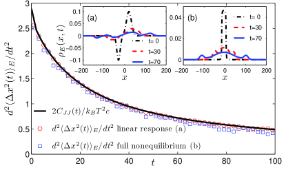
Figure 1: (Color online) Numerical validation of the main result in (9) for an FPU chain with a length $N=401$, specific heat $c=0.828$ at a dimensionless temperature $T=1$ Dimensionless.00.NULL . The red circles and the blue squares are the second derivative $d^{2}\langle\Delta x^{2}(t)\rangle_{E}/dt^{2}$ as obtained from the insets (a) and (b), respectively. The black solid line depicts the result for the total heat flux autocorrelation $\mathcal{C}_{JJ}(t)$, i.e. the rhs in (9). Insets: (a) energy diffusion along the FPU chain using the linear response result (6) with an initial small Hamiltonian perturbation $\eta(x)$ that is composed of two Gaussians of opposite weights; (b) nonequilibrium energy diffusion as obtained from an initial near equilibrium steady state. For further details see in Supplementary.00.NULL .

Anomalous energy diffusion vs. equilibrium heat flux correlation. The main result relating arbitrary ergodic energy diffusion to the equilibrium heat flux autocorrelation function can be obtained as follows: With the conservation of local energy $\partial_{t}h(x,t)+\partial_{x}j(x,t)=0$, we obtain Supplementary.00.NULL

$$\partial_{t}^{2}\mathcal{C}_{hh}(x,t)=\partial_{x}^{2}\mathcal{C}_{jj}(x,t).$$ (7)

Additionally, define $J_{L}=\int_{-L/2}^{L/2}j(x,t)dx$ to be the total heat flux for a 1D system of length $L$, we have

$$\mathcal{C}_{JJ}(t)\equiv\lim_{L\to\infty}\frac{1}{L}\left\langle J_{L}(t)J_{L}(0)\right\rangle_{eq}=\int_{-\infty}^{\infty}\mathcal{C}_{jj}(x,t)dx,$$ (8)

This autocorrelation function of total heat flux $\mathcal{C}_{JJ}$ is the central quantity that knowingly enters the Green–Kubo formula for normal heat conductivity Green.54.JCP ; Kubo.57.JPSJ ; Luttinger.64.PR ; Zwanzig.65.ARPC ; Visscher.74.PRA ; Allen.93.PRB .

Upon combining Eqs. (3), (6), (S24) and (8), we obtain the central result for the MSD:

$$\begin{split}\frac{d^{2}\langle\Delta x^{2}(t)\rangle_{E}}{dt^{2}}&\!=\!\frac{1}{\mathcal{N}}\!\!\iint\!\!x^{2}\frac{\partial^{2}\mathcal{C}_{hh}(x-x^{\prime},t)}{\partial t^{2}}{\eta(x^{\prime})}dxdx^{\prime}\\ &\!=\!\frac{2\mathcal{C}_{JJ}(t)}{k_{B}T^{2}c},\end{split}$$ (9)

where integration by parts has been used twice. This central equality constitutes an equation of motion for the MSD of general energy diffusion. The corresponding initial conditions are: ${\langle\Delta x^{2}(t=0)\rangle}_{E}=\iint x^{2}\mathcal{C}_{hh}(x-x^{\prime},0)\eta(x^{\prime})d{x}d{x^{\prime}}/\mathcal{N}-\big{(}\iint x\mathcal{C}_{hh}(x-x^{\prime},0)\eta(x^{\prime})d{x}d{x^{\prime}}/\mathcal{N}\big{)}^{2}$ and ${d\langle\Delta x^{2}(t)\rangle_{E}/dt}|_{t=0}=0$. It is only the initial value for $\langle\Delta x^{2}(t)\rangle_{E}$ that exhibits a dependence on the initially chosen energy perturbation. The vanishing initial speed follows from the fact that for an inertial dynamics $\mathcal{C}_{jj}(y,t)$ is an even function in time $t$, being continuously differentiable at time $t=0$. Therefore, any physically realistic energy diffusion process will start out as ballistic transport Huang.11.NP .

The numerical verification of the main finding in (9) is depicted in Fig. 1 for the theoretical archetype model of low-dimensional heat transfer, i.e. for an FPU chain, as detailed in Supplementary.00.NULL . Inset (a) is obtained by evaluating the linear response result (6) at dimensionless $T=1$ from an initial small perturbation $\eta(x)$ with a positive and a negative Gaussian weight. In inset (b), the full nonequilibrium energy diffusion is simulated from an initial, near equilibrium steady state using a preparation with heat baths of differing temperature. The energy diffusion proceeds after removing those heat baths. An ensemble of $4\times 10^{8}$ realizations are used to obtain the depicted nonequilibrium energy density distribution $\rho_{E}(x,t)$ in Fig. 1(b). The total heat flux autocorrelation function $\mathcal{C}_{JJ}(t)$ is obtained in thermal equilibrium at a temperature $T=1$ by averaging over an ensemble of $2\times 10^{9}$ realizations. The specific heat, $c=0.828$, is calculated analytically according to its definition. Very good agreement between theory and numerical experiments is obtained.

Let us recall the assumptions used in the derivation of this intriguing result: For the application of linear response theory the process is supposed to be sufficiently ergodic, implying that no nonstationary (i.e. aging) phenomena for long-time correlations are at work, thus ensuring manifest relaxation towards thermal equilibrium. This crucial ergodicity assumption rules out all anomalous energy diffusion processes that undergo aging, as it occurs in many continuous time random walk descriptions Metzler.00.PR ; Barkai.03.PRL ; Klafter.11.NULL ; Klafter.11.NULLa ; Sokolov.12.SM . Those models, however, lack a microscopic Hamiltonian basis. There exists, however, ergodic anomalous diffusion dynamics stemming from a Generalized Langevin equation (GLE) Goychuk.07.PRL ; Kubo.66.RPP ; Deng.09.PRE ; Goychuk.09.PRE ; Goychuk.11.NULL ; Siegle.11.EL ; Magdziarz.11.APNY ; Sokolov.12.SM . Likewise, microscopic Hamiltonian models involving homogeneous disordered lattices exhibit subdiffusive heat conductivity Dhar.01.PRL ; Roy.08.PRE . Our result (9) is robust against changes in the initial energy profile; it only affects the initial value of $\langle\Delta x^{2}(t)\rangle_{E}$. The main finding is restricted, however, to near equilibrium situations; matters may change drastically with perturbations of the system taken far away into nonequilibrium.

Relation to the Helfand scenario. Inspired by the Green-Kubo relation Green.54.JCP ; Kubo.57.JPSJ for normal transport, Helfand showed that the average over the canonical initial thermal equilibrium of all phase space coordinates of the squared displacement of the appropriate “Helfand moment”, i.e., $G_{L}(t)=\int_{-L/2}^{L/2}x\big{(}h(x,t)-\left\langle h(x)\right\rangle_{eq}\big{)}dx$, obeys $\langle[G_{L}(t)-G_{L}(0)]^{2}\rangle_{eq}/L=2\int_{0}^{t}(t-u)C_{JJ}(u)du$ Helfand.60.PR ; Viscardy.07.JCP ; Gaspard.08.JSMTaE . Therefore, taking the second time-derivative it follows with $L\rightarrow\infty$, that

$$\lim_{L\to\infty}\!\frac{d^{2}}{dt^{2}}\frac{\langle[G_{L}(t)-G_{L}(0)]^{2}\rangle_{eq}}{L}\!\equiv\!\frac{d^{2}\langle\Delta\mathcal{G}^{2}(t)\rangle_{eq}}{dt^{2}}\!=\!2\mathcal{C}_{JJ}(t).$$ (10)

Here, the initial conditions are $\langle\Delta\mathcal{G}^{2}(t=0)\rangle_{eq}=0$ and $d\langle\Delta\mathcal{G}^{2}(t)\rangle_{eq}/dt|_{t=0}=0$. Consequently, the scaled equilibrium average of the squared displacement of the Helfand moment, i.e., $\langle\Delta\mathcal{G}^{2}(t)\rangle_{eq}/k_{B}T^{2}c$, differs from $\langle\Delta x^{2}(t)\rangle_{E}$ by a constant shift, as determined by the initially chosen excess energy profile. In the absence of the main relation in (9), the mere result in (10) (with dimension $[\mathrm{length(energy)^{2}}]$) alone cannot provide the result for the spread $\langle\Delta x^{2}(t)\rangle_{E}$ of (anomalous) nonequilibrium energy diffusion. Observing the stated initial conditions, we next integrate (9) to yield the corollary

$$\frac{d\langle\Delta x^{2}(t)\rangle_{E}}{dt}=\int_{0}^{t}\frac{2\ \mathcal{C}_{JJ}(t^{\prime})}{k_{B}T^{2}c}dt^{\prime}=\frac{1}{k_{B}T^{2}c}\frac{d\langle\Delta\mathcal{G}^{2}(t)\rangle_{eq}}{dt}.$$ (11)

This finding can be interpreted as a time-local Helfand-like relation. This is so because in contrast to the ordinary Helfand relation for normal heat conductivity, i.e., $\kappa^{normal}=\langle\Delta\mathcal{G}^{2}(t)\rangle_{eq}/(2tk_{B}T^{2})$, no explicit time derivative enters Helfand.60.PR ; Viscardy.07.JCP ; Gaspard.08.JSMTaE . Put differently, (11) involves the time-local quantity $d\langle\Delta x^{2}(t)\rangle_{E}/dt$ (or $d\langle\Delta\mathcal{G}^{2}(t)\rangle_{eq}/dt$) rather than a finite time version $\langle\Delta x^{2}(t)\rangle_{E}/t$ (or $\langle\Delta\mathcal{G}^{2}(t)\rangle_{eq}/t$). This intriguing corollary (11) assumes an appealing form to establish the relationship between anomalous energy diffusion scaling and a generally anomalous scaling for the thermal conductivity $\kappa(L)$ obeying $J\sim\kappa(L)\Delta T/L$.

Normal energy diffusion. For normal energy diffusion the MSD increases asymptotically linearly in time, i.e., $\lim_{t\to\infty}\langle\Delta x^{2}(t)\rangle_{E}/t=2D_{E}$. $D_{E}$ is termed the thermal diffusivity. With time $t\to\infty$ in (11) we find

$$\kappa^{normal}\!=\!\!\!\int_{0}^{\infty}\!\frac{\mathcal{C}_{JJ}(t)}{k_{B}T^{2}}d{t}=\!\frac{c}{2}\!\lim_{t\to\infty}\!\!\frac{d\langle\Delta x^{2}(t)\rangle_{E}}{dt}\!=\!cD_{E}.$$ (12)

This is just the familiar Green-Kubo expression for normal heat conduction Helfand.60.PR ; Green.54.JCP ; Kubo.57.JPSJ ; Luttinger.64.PR ; Zwanzig.65.ARPC ; Visscher.74.PRA ; Allen.93.PRB . Arriving at this Green-Kubo relation it is important to recall that in all those cited derivations one implicitly or explicitly uses the validity of Fourier’s law, together with local thermal equilibrium; i.e. a transport behavior for steady state heat flux $j(x)=-\kappa\nabla{T(x)}$. For a small thermal bias $\Delta T$ the spatially constant gradient scales as $\nabla T(x)=\Delta T/L$. This in turn implies a length scaling for normal heat conductivity, $\kappa(L)=\kappa L^{\alpha=0}\equiv\kappa^{normal}$, being independent of system size. Normal heat diffusion being proportional to time $t$ thus implies with $\beta=1$ the self-consistent scaling relation, $\alpha=\beta-1=0$.

Superdiffusive energy diffusion. With ergodic superdiffusive energy diffusion obeying $\langle\Delta x^{2}(t)\rangle_{E}\sim t^{\beta}$, $1<\beta\leq 2$, the time-local Helfand relation (11) possesses no long time limit and the integral of $\mathcal{C}_{JJ}$ diverges as well. Therefore, no finite superdiffusive heat conductivity exists. The typical way out in practice Lepri.98.EL ; Narayan.02.PRL ; Lepri et al. (2003); Dhar (2008), however, is to consider a finite system of length $L$ and to formally introduce an upper cut-off signal time $t_{s}$ for heat transfer across the sample. In terms of a characteristic scale for the speed $v_{s}$ of phonon transport one sets $t_{s}\sim~{}L/v_{s}$; $v_{s}$ is commonly approximated by the speed of sound, being renormalized for nonlinearity Li.10.PRL . By adopting this reasoning, the use of the time-local Helfand relation (11) implies then an asymptotic behavior

$$\kappa_{L}^{{super}}\!\!\sim\!\frac{1}{k_{B}T^{2}}\!\int_{0}^{L/v_{s}}\!\!\!\mathcal{C}_{JJ}(t)d{t}=\!\frac{c}{2}\!\!\left.\frac{d\langle\Delta x^{2}(t)\rangle_{E}}{dt}\right|_{t\sim L/v_{s}}\!\!\!\!.$$ (13)

This finite-time Green–Kubo relation implies for the length-dependent superdiffusive heat conductivity $\kappa_{L}^{{super}}\sim L^{\alpha}$ the scaling relation

$$\alpha=\beta-1\;.$$ (14)

This result corroborates the relation derived for a specific case of a billiard model where the particles undergo an a priori assumed Lévy walk process Denisov.03.PRL ; Dhar.13.PRE .

Subdiffusive energy diffusion. Let us next consider an ergodic energy subdiffusion with $\langle\Delta x^{2}(t)\rangle_{E}\sim t^{\beta}$, $0<\beta<1$. From the main relation in (9) it follows that the total heat flux correlation $\mathcal{C}_{JJ}(t)\sim\beta(\beta-1)t^{\beta-2}$. With the relation for the exponent, i.e., $\delta=\beta-2<-1$, we find that $\mathcal{C}_{JJ}(t)$ remains integrable over the total time $[\,0,\infty)$. The time-local Helfand formula in (11) is thus applicable for $t\rightarrow\infty$; yielding

$$\kappa^{{sub}}=\lim_{t\to\infty}\frac{c}{2}\frac{d\langle\Delta x^{2}(t)\rangle_{E}}{dt}\sim\lim_{t\to\infty}t^{\beta-1}=0,$$ (15)

which indicates a perfect thermal insulator. — How does this vanishing of subdiffusive heat conductivity occur with increasing size $L$? — If we likewise may impose in (11) a finite cut-off time scale $t_{s}\propto L$ we find that ergodic heat subdiffusion occurs with $\kappa^{sub}\sim L^{\alpha}$, $-1<\alpha=\beta-1<0$.

Conclusion. With this work we studied anomalous heat diffusion in the absence of ergodicity breaking. The main finding in (9) relates dynamically the acceleration of the nonequilibrium energy MSD directly to the equilibrium autocorrelation $\mathcal{C}_{JJ}(t)$ of the total heat flux. Equivalently, this result assumes the form of a time-local Helfand relation as specified with (11). Given the premise that anomalous stationary heat flux follows a behavior in terms of an anomalous heat conductivity, i.e. $\kappa(L)\sim L^{\alpha}$, then implies the scaling, $\alpha=\beta-1$. Because (9) applies for all times $t$, it can be invoked as well for those intermediate cases where an anomalous, length-dependent heat conductivity occurs over a finite size Zhang.05.JCP ; Henry.08.PRL ; Henry.09.PRB ; Nika.09.APL ; Yang.10.NT ; Lindsay.10.PRB ; Lindsay.11.PRB ; Nika.12.NL ; Liu.12.PRB .

The similarity between the global Helfand moment scenario used for normal diffusion in Ref. Helfand.60.PR with the time-local result in (11) suggests analogous relations as in (9) to hold for other anomalous diffusion processes. Particularly, what comes to mind is unbiased, anomalous particle diffusion $x_{p}(t)$. Unlike for energy diffusion in solid phases, the position increments, i.e., $(x_{p}(t)-x_{p}(s))=\int_{s}^{t}{\dot{x}}_{p}(t^{\prime})dt^{\prime}$, are now given in terms of the particle velocity $\dot{x}_{p}(t)$. Indeed with ergodic anomalous diffusion obtained from an equilibrium GLE-dynamics Deng.09.PRE ; Goychuk.09.PRE ; Goychuk.11.NULL ; Siegle.11.EL ; Magdziarz.11.APNY ; Sokolov.12.SM : with ${\dot{x}}_{p}=v(t)$ and $\langle v(t)\rangle_{eq}=0$, $m\langle v^{2}(t)\rangle_{eq}=k_{B}T$, it readily follows that (9) implies $d^{2}\langle x_{p}^{2}(t)\rangle/dt^{2}=2\langle v(t)v(0)\rangle_{eq}$ for all times $t$ note .

In this supplementary material we detail in a more explicit manner our theoretical and numerical analysis used in deriving our main results and provide additional insight as needed in our study.

I System under study and definitions

In the following we assume that no particle and charge exchanges assist the energy transport. We thus consider a 1D system given by the Hamiltonian:

$$H=\sum_{n}H_{n}(X),$$ (S1)

where $X$ denotes the complete set of canonical phase space coordinates $(\{q_{i}\},\{p_{i}\})$ describing the microscopic system dynamics. $H(X)$ is composed as a sum of the corresponding discrete, local Hamiltonian of the $n$’th particle dynamics with the interaction between neighboring particles being short ranged. In a space-continuous description this total Hamiltonian then assumes the form as an integral over a local energy density $h(x)$; i.e.,

$$H=\int h(x)dx,\quad\quad h(x)=\sum_{n}H_{n}\delta(x-q_{n}).$$ (S2)

Given this local energy density the corresponding local energy current obeys the condition of local energy conservation,

$$\partial_{t}h(x)+\partial_{x}j(x)=0\;,$$ (S3)

or its discrete correspondence. A more detailed discussion and the specific definitions in terms of the system parameters and interaction potentials can be found in the comprehensive two reviews Lepri et al. (2003); Dhar (2008).

II Evolution of the excess energy distribution

Next, we derive the time-evolution of the excess energy distribution, using the discrete version. The corresponding result for the space-continuous version follows in a straightforward manner.

In thermal equilibrium characterized by the temperature $T$ the probability for the phase space coordinates obeys with inverse temperature $\beta_{T}=1/(k_{B}T)$ the canonical form

$$f_{eq}=\frac{1}{Z}e^{-\beta_{T}H}\quad\quad\mathrm{with}\quad\quad Z=\int e^{-\beta_{T}H}d\Gamma\;,$$ (S4)

where $d\Gamma=dq_{1}\cdots dp_{1}\cdots$. For a prepared nonequilibrium initial phase space probability the time evolution is governed by the Liouville equation,

$$\frac{\partial}{\partial t}f(t)=Lf=\left\{H,f\right\}\;,$$ (S5)

where $\left\{A,B\right\}$ denotes the Poisson bracket

$$\left\{A,B\right\}=\sum_{i}\left(\frac{\partial A}{\partial q_{i}}\frac{\partial B}{\partial p_{i}}-\frac{\partial A}{\partial p_{i}}\frac{\partial B}{\partial q_{i}}\right).$$ (S6)

Next we introduce a small perturbation $H^{\prime}$ of the Hamiltonian, reading:

$$H^{\prime}=-\sum_{n}\eta_{n}H_{n}\;.$$ (S7)

Physically this means that we prepare a nonequilibrium probability, i.e., $f_{neq}(t=0)$, by suddenly switching off at $t=0$ the quenched Hamiltonian $H_{T}=H+H^{\prime}$, which is assumed to have acted since infinite past. Put differently, the initial-value problem we solve has an initial probability prepared in such a displaced, frozen-equilibrium ensemble probability, whose future time evolution $f_{neq}(t),t>0$ is governed by the unperturbed Liouvillian $L$. It thus reads

$$f_{neq}(t=0)=\frac{1}{Z^{\prime}}e^{-\beta_{T}(H+H^{\prime})}\quad\quad\mathrm{with}\quad\quad Z^{\prime}=\int e^{-\beta_{T}(H+H^{\prime})}d\Gamma\;.$$ (S8)

Using that $H^{\prime}$ is small, we can expand $Z^{\prime}$ to linear order, yielding

$$Z^{\prime}=\int e^{-\beta_{T}H}(1-\beta_{T}H^{\prime})d\Gamma=Z\left(1-\frac{1}{Z}\int e^{-\beta_{T}H}\beta_{T}H^{\prime}d\Gamma\right)=Z(1-\beta_{T}\left\langle H^{\prime}\right\rangle).$$ (S9)

As time evolves this nonequilibrium probability for $t>0$ assumes the formal solution

$$\begin{split}f_{neq}(t)&=e^{tL}f_{neq}(t=0)=\frac{1}{Z^{\prime}}e^{tL}e^{-\beta_{T}H^{\prime}}e^{-\beta_{T}H}\\ &\approx\frac{1}{Z}(1+\beta_{T}\left\langle H^{\prime}\right\rangle_{eq})e^{tL}(1-\beta_{T}H^{\prime})e^{-\beta_{T}H}\approx e^{tL}(1-\beta_{T}\Delta H^{\prime})f_{eq}\\ &=f_{eq}-\beta_{T}e^{tL}\Delta H^{\prime}f_{eq},\end{split}$$ (S10)

where for any quantity $A$, we define $\Delta A=A-\left\langle A\right\rangle_{eq}$. The expectation value then for $H_{n}(\{q_{i}\},\{p_{i}\})$ reads

$${\langle H_{n}(t)\rangle}_{neq}=\int H_{n}f_{neq}(t)d\Gamma=\left\langle H_{n}\right\rangle_{eq}-\beta_{T}\int H_{n}e^{tL}\Delta H^{\prime}f_{eq}d\Gamma.$$ (S11)

The linear response in Eq. (S11) can thus be cast in terms of a stationary equilibrium correlation function of energy-energy fluctuations, reading

$$\delta{\langle H_{n}(t)\rangle}_{neq}={\langle H_{n}(t)\rangle}_{neq}-\left\langle H_{n}(t)\right\rangle_{eq}=-\beta_{T}\left\langle H_{n}(t)\Delta H^{\prime}(0)\right\rangle.$$ (S12)

Using the result in (S7) we obtain

$$\Delta{\langle H_{n}(t)\rangle}_{neq}=\sum_{i}\frac{\eta_{i}}{k_{B}T}\left\langle\Delta H_{n}(t)\Delta H_{i}(0)\right\rangle.$$ (S13)

Similarly, the spatial-continuous version is analogously given by the initial nonequilibrium probability density

$$f_{neq}(t=0)=\frac{1}{Z^{\prime}}e^{-\beta_{T}\int[1-\eta(x)]h(x)dx},$$ (S14)

yielding for time evolution of the excess energy density:

$$\delta{\langle h(x,t)\rangle}_{neq}=\frac{1}{k_{B}T}\int\eta(x^{\prime})\left\langle\Delta h(x,t)\Delta h(x^{\prime},0)\right\rangle dx^{\prime}.$$ (S15)

Equation (S13) remains valid as well for the system formally connected to to generalized Langevin heat baths, see in Grabert et al. (1977, 1980). In such a case, the Liouville equation should be replaced by a corresponding, typically non-Markovian, generalized master equation operator which determines the evolution of phase space density. Therefore, the derivation are the same by replacing the Liouville operator $L$ with a generalized master operator; i.e., $L\to L_{\mathrm{GME}}$ Grabert et al. (1978).

III Heat capacity and heat-flux autocorrelation function

In this section, we first demonstrate the relation

$$\lim_{L\to\infty}\int_{-L/2}^{L/2}\mathcal{C}_{hh}(x,0)dx=k_{B}T^{2}c\;,$$ (S16)

where $c$ denotes the specific volumetric heat capacity. Consider first a continuous finite system with length $L$ in thermal equilibrium. Then the total system energy

$$E_{L}=\int_{-L/2}^{L/2}h(x,t)dx,$$ (S17)

fluctuates in time. From a thermal equilibrium statistics, the variance of this energy fluctuation obeys

$$\left\langle\Delta E_{L}\Delta E_{L}\right\rangle=k_{B}T^{2}C=k_{B}T^{2}cL\;,$$ (S18)

where $C=cL$ is the total heat capacity for the system of size $L$.

For the spatial correlation of the equilibrium energy density $\Delta h(x,t)$ we find for (S18) with temporal invariance and observing the fact that this equilibrium correlation is a symmetric function of its arguments $(x,x^{\prime})$, i.e., $\mathcal{C}_{hh}(x,0;x^{\prime},0)=\mathcal{C}_{hh}(x^{\prime},0;x,0)$, thus allowing the restriction of integration to the domain $x^{\prime}>x$ by doubling the integral:

$$\int_{-L/2}^{L/2}dx\int_{-L/2}^{L/2}dx^{\prime}\left\langle\Delta h(x,t)\Delta h(x^{\prime},t)\right\rangle=\int_{-L/2}^{L/2}dx\int_{-L/2}^{L/2}dx^{\prime}\mathcal{C}_{hh}(x,0;x^{\prime},0)=2\int_{-L/2}^{L/2}dx\int_{x}^{L/2}dx^{\prime}\mathcal{C}_{hh}(x,0;x^{\prime},0).$$ (S19)

We now introduce the difference variable $y=x^{\prime}-x$ and use with spatial homogeneity that $\mathcal{C}_{hh}(y,t)=\mathcal{C}_{hh}(-y,t)$, followed by a change of order of integration, yielding

$$\begin{split}2\int_{-L/2}^{L/2}dx\int_{x}^{L/2}dx^{\prime}\;\mathcal{C}_{hh}(x,0;x^{\prime},0)&=2\int_{-L/2}^{L/2}dx\int_{0}^{L/2-x}dy\;\mathcal{C}_{hh}(x,0;x+y,0)\\ &=2\int_{-L/2}^{L/2}dx\int_{0}^{L/2-x}dy\;\mathcal{C}_{hh}(y,0)\\ &=2\int_{0}^{L}dy\;\mathcal{C}_{hh}(y,0)\int_{-L/2}^{L/2-y}dx\\ &=2L\int_{0}^{L}dy\;\mathcal{C}_{hh}(y,0)\Big{(}1-\frac{y}{L}\Big{)}.\end{split}$$ (S20)

For finite time $t$ the integral $\int_{0}^{\infty}\mathcal{C}_{hh}(y,t)dy$ must exist. The reasoning goes as follows. Because the spatial-temporal correlation function $\mathcal{C}_{hh}(x,t)$ results as the response to a sharp perturbation at position $x^{\prime}=0$ at $t=0$, as shown with (S15) by considering formally the perturbation $\eta(x^{\prime})=\delta(x^{\prime})$. In physical realistic materials, it always requires finite time to reach the cause at position $x$ due to an applied initial perturbation at $x=0$; i.e. there is always only a finite speed $v_{s}$ available for information transfer. In our case, this finite speed for information transfer is characterized by the sound speed $v_{s}$. Thus, $\mathcal{C}_{hh}(x,t)$ vanishes outside of the causal “sound cone”, given by $|x|>v_{s}t$. This consequently implies the convergence of $\int_{0}^{\infty}\mathcal{C}_{hh}(y,0)dy$. It then follows that for arbitrary finite $t$

$$\lim_{L\to\infty}\int_{0}^{L}dy\;\frac{y}{L}\mathcal{C}_{hh}(y,t)=0.$$ (S21)

Noting that $2\int_{0}^{\infty}dy\;\mathcal{C}_{hh}(y,0)=\int_{-\infty}^{\infty}dy\;\mathcal{C}_{hh}(y,0)$ and the division in (S18) by $L$ we find in this limit of large system size $L$

$$\int_{-\infty}^{\infty}\mathcal{C}_{hh}(x,0)dx=\lim_{L\to\infty}\frac{1}{L}\left\langle\Delta E_{L}\Delta E_{L}\right\rangle=k_{B}T^{2}c\;.$$ (S22)

This shows the validity of the relation in (S16). At best it is only at critical points with diverging specific volumetric heat capacity $c$ that $\int_{0}^{\infty}\mathcal{C}_{hh}(y,0)dy$ may not converge.

Using the change $h(x,t)\to$ $j(x,t)$ (the energy current density) and $E_{L}\to$ $J_{L}$ (the the total heat flux), the same way of reasoning then yields the result that

$$C_{JJ}(t)=\lim_{L\to\infty}\frac{1}{L}\left\langle J_{L}(t)J_{L}(0)\right\rangle=\int_{-\infty}^{\infty}\mathcal{C}_{jj}(x,t)dx\;.$$ (S23)

IV Relation between energy density correlation and heat flux density correlation

Let us show that

$$\frac{\partial^{2}\mathcal{C}_{hh}(x,t)}{\partial t^{2}}=\frac{\partial^{2}\mathcal{C}_{jj}(x,t)}{\partial x^{2}}.$$ (S24)

Using local conservation of energy current we multiply Eq. (S3) by $h(x^{\prime},t^{\prime})$ and $j(x^{\prime},t^{\prime})$ respectively, and take the ensemble averages:

$$\partial_{t}\left\langle h(x,t)h(x^{\prime},t^{\prime})\right\rangle+\partial_{x}{\left\langle j(x,t)h(x^{\prime},t^{\prime})\right\rangle} = 0,$$ (S25)

$$\partial_{t^{\prime}}\left\langle h(x^{\prime},t^{\prime})j(x,t)\right\rangle+\partial_{x^{\prime}}{\left\langle j(x^{\prime},t^{\prime})j(x,t)\right\rangle} = 0.$$ (S26)

In the second line, we interchanged $(x,t)\to(x^{\prime},t^{\prime})$.

By performing $\partial_{t^{\prime}}$ to Eq. (S25) and $\partial_{x}$ to Eq. (S26), we obtain

$$\frac{\partial^{2}}{\partial t\partial t^{\prime}}\left\langle h(x,t)h(x^{\prime},t^{\prime})\right\rangle=\frac{\partial^{2}}{\partial x\partial x^{\prime}}\left\langle j(x,t)j(x^{\prime},t^{\prime})\right\rangle$$ (S27)

The time-translational invariance implies that $\left\langle h(x,t)h(x^{\prime},t^{\prime})\right\rangle=\left\langle h(x,t-t^{\prime})h(x^{\prime},0)\right\rangle$. Therefore

$$\frac{\partial^{2}}{\partial t\partial t^{\prime}}\left\langle h(x,t)h(x^{\prime},t^{\prime})\right\rangle=-\frac{\partial^{2}}{\partial t^{2}}\left\langle h(x,t)h(x^{\prime},t^{\prime})\right\rangle.$$ (S28)

For a spatially homogeneous system, this simplifies to yield $\left\langle j(x,t)j(x^{\prime},t^{\prime})\right\rangle=\mathcal{C}_{jj}(x-x^{\prime},t-t^{\prime})$ so that

$$\frac{\partial^{2}}{\partial x\partial x^{\prime}}\left\langle j(x,t)j(x^{\prime},t^{\prime})\right\rangle=-\frac{\partial^{2}}{\partial x^{2}}\left\langle j(x,t)j(x^{\prime},t^{\prime})\right\rangle\;.$$ (S29)

Observing (S28) and (S29) we find the relation in (S24).

V Conservation of excess energy and time independence for mean of energy diffusion

In this section, we show that for a homogeneous system, the total excess energy

$$\delta E(t)=\int\delta{\langle h(x,t)\rangle}_{neq}dx=\frac{1}{k_{B}T}\iint\mathcal{C}_{hh}(x-x^{\prime},t)\eta(x^{\prime})dx^{\prime}dx,$$ (S30)

remains conserved. To show this, we take the time derivative twice, which gives with integration by parts and together with Eq. (S24)

$$\frac{d^{2}\delta E(t)}{dt^{2}}=\frac{1}{k_{B}T}\iint\frac{\partial^{2}\mathcal{C}_{hh}(x-x^{\prime},t)}{\partial t^{2}}\eta(x^{\prime})dx^{\prime}dx=\frac{1}{k_{B}T}\iint\frac{\partial^{2}\mathcal{C}_{jj}(x-x^{\prime},t)}{\partial x^{2}}\eta(x^{\prime})dx^{\prime}dx=0\;.$$ (S31)

Thus, the first time derivative is a constant. On the other hand, at $t=0$, we obtain

$$\frac{d\delta E(0)}{dt}=\frac{1}{k_{B}T}\iint\left.\frac{\partial\mathcal{C}_{hh}(x-x^{\prime},t)}{\partial t}\right|_{t=0}\eta(x^{\prime})dx^{\prime}dx.$$ (S32)

Note that for any inertial dynamics $\mathcal{C}_{hh}(x-x^{\prime},t)$ is an even function of $t$, being continuously differentiable at $t=0$. Therefore, the rhs vanishes, yielding $d\delta E(t)/{dt}$ identically zero, implying that $\delta E(t)$ is conserved.

Using a similar reasoning it follows that the first moment of the excess energy ${\langle x\rangle}_{E}=\int x\rho_{E}(x,t)dx$ remains constant.

VI Numerical details

Using dimensionless units Unit.00.NULL the Hamiltonian of the Fermi-Pasta-Ulam (FPU) lattice reads:

$$H=\sum_{i}\left[\frac{1}{2}p^{2}_{i}+\frac{1}{2}(q_{i+1}-q_{i})^{2}+\frac{1}{4}(q_{i+1}-q_{i})^{4}\right]\;.$$ (S33)

Here, the set ${q_{i}}$ denotes the relative displacement with respect to the equilibrium position $ia$ and ${p_{i}}$ denotes the momentum for the $i$-th atom, where $a$ is the lattice constant which can be scaled to unity, i.e., $a=1$ Unit.00.NULL . We further use periodic boundary conditions; i.e., $q_{N+1}=q_{1}$. The lattice length is $L=Na$ with $N=401$. The local energy $H_{i}(t)$ is then chosen as:

$$H_{i}(t)=\frac{1}{2}p^{2}_{i}+\frac{1}{2}\big{[}V(q_{i}-q_{i-1})+V(q_{i+1}-q_{i})\big{]};\quad V(x)=\frac{1}{2}x^{2}+\frac{1}{4}x^{4}.$$ (S34)

For convenience, the atom indexes are chosen as $i=-200,\cdots,200$. In the simulation, the dimensionless time step size is set to $\tau=0.05$.

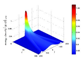
Figure 2: (Color online) The time evolution of the nonequilibrium energy density for a manifest near equilibrium energy diffusion dynamics.

To evaluate both, $C_{hh}(x,t)$ in linear response, Eq. (S13), and the heat flux autocorrelation function $C_{JJ}(t)$ in thermal equilibrium, we first apply Langevin heat baths at temperature $T=1$ to all atoms. The velocity-Verlet algorithm is used. Doing so does prepare the canonical equilibrium state. After all transients have died out, the heat baths are removed. Then a fourth order symplectic SABA₂C algorithm Laskar.01.CMDA is used to integrate the equations of motion and the corresponding correlation functions are calculated. The final correlation function is based on an average over $2\times 10^{9}$ realizations. For our illustration in Fig. 1(a), the excess energy distribution are based on Eq. (S13), using an initial excess energy profile $\eta_{i}$, being composed of two Gaussian peaks, one with positive and one with negative weight; i.e. we set:

$$\eta_{i}=10^{-3}\;\Big{[}\exp{\left(-\frac{(i-20)^{2}}{2\times 12^{2}}\right)}-\exp{\left(-\frac{(i+30)^{2}}{2\times 8^{2}}\right)}\Big{]}\;.$$ (S35)

To simulate a full nonequilibrium energy diffusion, we first prepare the system in a nonequilibrium steady state near a reference temperature $T=1$. Specifically, we apply Langevin heat baths to all atoms with different temperatures:

$$T_{i}=\begin{cases}1.2&\mathrm{for}\ -10\leq i\leq 10;\\ 1.0&\mathrm{otherwise}.\end{cases}$$ (S36)

We use velocity-Verlet algorithm and run for $1\times 10^{7}$ steps to reach the nonequilibrium steady state. Then all the heat baths are removed and the energy profiles are calculated up to time $t=100$ using the fourth order symplectic SABA₂C algorithm. An ensemble of $4\times 10^{8}$ realizations are used to evaluate the time evolution of the nonequilibrium energy density $\left\langle H_{i}(t)\right\rangle_{neq}$ as depicted in Fig. (2). The normalized energy distribution $\rho_{E}(x,t)$ is calculated using

$$\rho_{E}(x=i,t)=\frac{\left\langle H_{i}(t)\right\rangle_{neq}-\left\langle H_{i}\right\rangle}{\sum_{i}\left[\left\langle H_{i}(t)\right\rangle_{neq}-\left\langle H_{i}\right\rangle\right]},$$ (S37)

where the reference energy density $\left\langle H_{i}\right\rangle$ is set to the average energy density at reference temperature $T=1$, which equals $0.867$, see in Eq. (S40) below.

Finally, the MSD is calculated using Eq. (3) in the main article and the second time derivate is calculated using the formula

$$\frac{d^{2}f(t)}{dt^{2}}=\frac{f(t+\Delta t)-2f(t)+f(t-\Delta t)}{\Delta t^{2}}$$ (S38)

with $\Delta t=20h=1$.

The volumetric specific heat $c$ is calculated analytically according to its definition

$$c=\frac{d\left\langle H_{i}(T)\right\rangle}{dT},$$ (S39)

where $\left\langle H_{i}(T)\right\rangle$ is the average energy per particle at temperature $T$, which can be calculated as Unit.00.NULL

$$\left\langle H_{i}(T)\right\rangle=\left\langle e_{kinetic}\right\rangle+\left\langle e_{potential}\right\rangle=\frac{1}{2}T+\frac{\int V(x)e^{-V(x)/T}dx}{\int e^{-V(x)/T}dx}.$$ (S40)

For $T=1$, we obtain $\left\langle H_{i}(T)\right\rangle=0.867$ and $c=0.828$.

References

- Lepri et al. (2003) S. Lepri, R. Livi, and A. Politi, Phy. Rep. 377, 1 (2003).
- Dhar (2008) A. Dhar, Adv. Phys. 57, 457 (2008).
- Grabert et al. (1977) H. Grabert, P. Talkner, and P. Hänggi, Z. Physik B 26, 389 (1977).
- Grabert et al. (1980) H. Grabert, P. Hänggi, and P. Talkner, J. Stat. Phys. 22, 537 (1980).
- Grabert et al. (1978) H. Grabert, P. Hänggi, and P. Talkner, Phys. Lett. A 66, 255 (1978).
- (6) Following Li.12.RMP , we choose the atom mass , the lattice constant , the force constant and the Boltzmann constant as the four basic units to scale all physical quantities involved to dimensionless quantities.
- (7) N. Li, J. Ren, L. Wang, G. Zhang, P. Hänggi and B. Li, Rev. Mod. Phys. 84, 1045 (2012).
- (8) J. Laskar and P. Robutel, Celest. Mech. Dyn. Astron. 80, 39 (2001).