Horizontal flow fields observed in
Hinode G-band images

Abstract

Context. The interaction of plasma motions and magnetic fields is an important mechanism, which drives solar activity in all its facets. For example, photospheric flows are responsible for the advection of magnetic flux, the redistribution of flux during the decay of sunspots, and the built-up of magnetic shear in flaring active regions.

Aims. Systematic studies based on G-band data from the Japanese Hinode mission provide the means to gather statistical properties of horizontal flow fields. This facilitates comparative studies of solar features, e.g., G-band bright points, magnetic knots, pores, and sunspots at various stages of evolution and in distinct magnetic environments, thus, enhancing our understanding of the dynamic Sun.

Methods. We adapted Local Correlation Tracking (LCT) to measure horizontal flow fields based on G-band images obtained with the Solar Optical Telescope on board Hinode. In total about 200 time-series with a duration between 1–16 h and a cadence between 15–90 s were analyzed. Selecting both a high-cadence ($\Delta t=15$ s) and a long-duration ($\Delta T=16$ h) time-series enabled us to optimize and validate the LCT input parameters, hence, ensuring a robust, reliable, uniform, and accurate processing of a huge data volume.

Results. The LCT algorithm produces best results for G-band images having a cadence of 60–90 s. If the cadence is lower, the velocity of slowly moving features will not be reliably detected. If the cadence is higher, the scene on the Sun will have evolved too much to bear any resemblance with the earlier situation. Consequently, in both instances horizontal proper motions are underestimated. The most reliable and yet detailed flow maps are produced using a Gaussian kernel with a size of 2560 km $\times$ 2560 km and a full-width-at-half-maximum (FWHM) of 1200 km (corresponding to the size of a typical granule) as sampling window.

Conclusions. Horizontal flow maps and graphics for visualizing the properties of photospheric flow fields are typical examples for value-added data products, which can be extracted from solar databases. The results of this study will be made available within the ‘small projects’ section of the German Astrophysical Virtual Observatory (GAVO).

1 Introduction

Data from space do not suffer the deleterious effects of Earth’s turbulent atmosphere, which blur and distort images so that features might fade into obscuration, making it difficult to follow them from image to image. The huge volume of Hinode G-band images with good spatial resolution, cadence, and coverage provide time-series of consistent quality to quantify photospheric proper motions, which can be used in comparative studies.

Various techniques have been developed in the past decades to measure horizontal proper motions on the solar surface. Basically, they can be divided in two classes. The first class includes Feature Tracking (FT) methods, which follow the footprints of individual features in images of a time-series (see e.g. Strous, 1995). Tracking facular points of opposite magnetic polarity in an emerging flux region effectively demonstrated the potential of FT techniques (Strous et al., 1996). However, the image processing steps (segmentation, labeling, and identification) rely on prior knowledge about the object under investigation. Therefore, FT methods seem to be better suited for case studies rather than bulk processing of huge data volumes, where the reduction of dimensionality is a desirable feature. The balltracking method developed by Potts et al. (2004) can also be subsumed under FT techniques, since artificial tracer particles are introduced to follow the footprints of local intensity minima. The ball tracking method works well for granulation so that it is a good choice for the characterization of supergranulation (Potts & Diver, 2008). Nevertheless, it might introduce a scale dependence, when tracking on other (small-scale) features such as bright points, penumbral grains, and umbral dots.

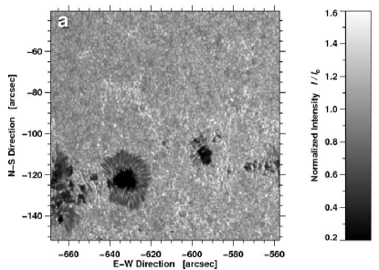
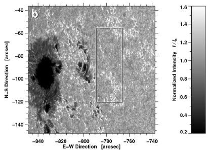
Figure 1: Calibrated G-band images of active regions (a) NOAA 10960 and (b) NOAA 10930 observed on 2007 June 4 and 2006 December 7, respectively. The FOV is $111\arcsec\times 111\arcsec$. The annotation of the axes refers to heliocentric coordinates given in seconds of arc. The region in the rectangular white box is used for further analysis zooming in on a quiet Sun region containing numerous G-band bright points outlining supergranular boundaries. The images were normalized such that the mode of the quiet Sun intensity distribution corresponds to unity.

The second class is based on Local Correlation Tracking (LCT), where displacement vectors are derived by cross-correlating small regions in consecutive images of a time-series. The principles of LCT are laid out in the seminal work of November & Simon (1988). Leaving behind the underlying velocity assumption of LCT Schuck (2006) developed a technique to track optical flows named the differential affine velocity estimators (DAVE). Chae & Sakurai (2008) presented a formulation of the non-linear case and called it accordingly the nonlinear affine velocity estimators (NAVE). These authors also provide a detailed parameter study of LCT, DAVE, and NAVE based on images reflecting analytical solutions of the continuity equation as well as on magnetogram data from Hinode and MHD simulations. Similarly, Welsch et al. (2007) compared these velocity inversion techniques based on MHD simulations, where the velocity field is known.

Various other technical aspects have to be considered while implementing techniques for optical flow tracking. Since interpolations are required in the various data reduction steps, we refer to Potts et al. (2003), who describe the systematic errors, which can be introduced by unsuitable interpolation schemes. More recently, Löfdahl (2010) discussed image-shift measurements in the context of solar wavefront sensors, which are also applicable to the LCT implementations.

Hinode G-band images offer an excellent opportunity for systematic statistical studies of flow fields, because of their uniform quality in the absence of seeing distortions, thus alowing us to directly compare flow fields in different solar settings. In Sect. 2, we introduce the high-cadence and long-duration data sets, which are used to find the optimal parameters for computing LCT maps based on time-series of Hinode G-band images. The implementation of the algorithm is described in Sect. 3. Section 4 presents the results of this parameter study justifying our choice of LCT parameters, which will be used to create value-added data to complement the Hinode database. The most important parameters are summarized in Sect. 5, which also introduces some of the future uses of such a database.

2 Observations

Images obtained in the Fraunhofer G-band (bandhead of the CH molecule at $\lambda$430.5 nm) have high contrasts, and small-scale magnetic features can be simply identified with bright points (Berger et al., 1995). Despite the observational advantages of such “proxy-magnetometry” (Leenaarts et al., 2006), the theoretical description of the molecular line formation process is far from easy (cf. Sánchez Almeida et al., 2001; Steiner et al., 2001; Schüssler et al., 2003). LCT techniques, however, can take full advantage of the high contrast and the rich structural contents of G-band images. On Hinode (Kosugi et al., 2007) such observations are carried out by the Broad-band Filter Imager (BFI) of the Solar Optical Telescope (SOT, Tsuneta et al., 2008).

Our initial selection criteria were that at least 100 G-band images had to be recorded on a given day, which should have additionally a cadence of better than 100 s. It turned out that these criteria restricted us to data with only half the spatial resolution (0.11″ pixel^-1), where $2\times 2$ pixels were binned into one. In total 48 data sets with $2048\times 1024$ pixels and 153 data sets with $1024\times 1024$ pixels were selected for further analysis. The time intervals covered by these data sets range from one to 16 hours. The bulk statistical analysis will be presented in forthcoming publications. Here, we will discuss in detail the LCT algorithm and justify our choice of input parameters. For this purpose, we selected two data sets: one with a high cadence and another one with a long duration. In addition, we picked a data set without binning to study the dependence of flow maps on the spatial resolution of the input data.

2.1 High-cadence sequence

LCT depends on several input parameters such as the time interval between successive images and the sampling window’s size and form. We analyzed an one-hour time-series with a cadence of 15 s to validate the intrinsic accuracy of the LCT algorithm. The data were captured from 14:27–15:27 UT on 2007 June 4 (see Fig. 1a). The time-series contains 238 images with $1024\times 1024$ pixels. The observations were centered on active region NOAA 10960, which was located on the solar disk at heliocentric coordinates E630″ and S125″ ($\mu=0.75$). The active region was in the maximum growth phase and had a complex magnetic field configuration. NOAA 10960 was classified as a $\beta\gamma\delta$-region and was the source of many M-class flares including a major M8.9 flare at 05:06 UT on 2007 June 4, which has been analyzed in a multi-wavelength study by Kumar et al. (2010).

2.2 Long-duration sequence

Solar features evolve on different time scales from about five minutes for granulation to several tens of hours for supergranulation. Obviously, the time over which individual LCT maps are averaged plays a decisive role in the interpretation of such average flow maps. Hence, we selected a time-series with 16 hours of continuous data captured on 2006 December 7 (see Fig. 1b). This long-duration sequence starts at 02:30 UT and ends at 18:30 UT. It includes 960 images with $1024\times 1024$ pixels and has a cadence of 60 s. Due to memory constrains imposed by the subsonic filtering we choose an area of $210\times 595$ pixels centered on a region with granulation and G-band bright points (white box Fig. 1b). This region is to the west of active region NOAA 10930 located at heliocentric coordinates E777″and S88″ ($\mu=0.59$). The sunspot group was classified as a $\beta\gamma\delta$-region exhibiting a complex magnetic field topology and producing numerous C-, M-, and X-class flares. This region has been extensively studied, especially around the time of an X3.4 flare on 2006 December 13 (e.g., Schrijver et al., 2008). LCT techniques were used by Tan et al. (2009) to study horizontal proper motions associated with penumbral filaments in a rapidly rotating $\delta$-spot.

2.3 High-spatial resolution sequence

Only a few data sets of G-band images exist with the full spatial resolution of 0.055″ pixel^-1 and a cadence suitable for LCT. We selected a one-hour time-series, which was acquired starting at 04:00 UT on 2006 November 26. This high-spatial resolution sequence contains 118 images with $2048\times 2048$ pixels and has a time cadence of about 30 s. The observations were centered on a quiet Sun region near disk center at heliocentric coordinates E108″ and S125″ ($\mu=0.99$) containing only a few G-band bright points and no major magnetic flux concentrations.

3 Implementation of the LCT algorithm

3.1 Preprocessing of the G-band images

The data analysis is carried out in the Interactive Data Language (IDL). Data sets are split in 60-minute sequences with 30 min overlap between consecutive sequences. In preparation for the LCT algorithm basic data calibration is performed, which consists of dark current subtraction, correction of gain, and removal of spikes caused by high energy particles. Figure 1 contains sample G-band images for both the high-cadence and long-duration data sets after basic calibration. After initial data calibration, the geometric foreshortening is corrected and images are resampled in a regular grid with spacing of 80 km $\times$ 80 km, i.e., the images appear as if observed at the center of the solar disk. Residual effects of projecting the surface of a sphere onto a plane are neglected, since the FOV of the G-band images is still relatively small. A grid size of 80 km was chosen so that the fine structure contents of the G-band images are not diminished. Pixels close to the solar limb are projected onto several pixels in planar coordinates. Thus, the accuracy of the flow maps at these locations is not as good as for locations close to disk center.

In a 60-minute sequence are $l=0,1,2,\ldots,L-1$ calibrated and deprojected images, where $L$ is the total number of images in a particular sequence. For an image with $N\times M$ pixels the intensity distribution is represented by $i(x,y)$ with $x=x_{0},x_{1},\ldots,x_{N-1}$ and $y=y_{0},y_{1},\ldots,y_{M-1}$ as pixel coordinates. The indices are typically dropped to ease the notation. The data processing makes extensive use of the Fast Fourier Transform (FFT). The FFT of the intensity distribution $i(x,y)$ is simply denoted by ${\cal F}(i(x,y))$.

3.2 Aligning the images within a time-series

In principle, images could be aligned using the pointing information of the spacecraft. However, we calculate shifts between consecutive images $i_{l-1}(x,y)$ and $i_{l}(x,y)$ by computing the cross-correlation using only the central part of the images, which is half of the original image size. These shifts are then applied in succession to align all images with respect to the first image using cubic spline interpolation with subpixel accuracy. The signature of the 5-minute oscillation is removed from the time-series by applying a 3D Fourier filter. This filter, sometimes called a subsonic filter, has a cut-off velocity of $c_{s}\approx 8$ km s^-1 corresponding to the photospheric sound speed. Since the subsonic filter uses a 3D Fourier transform some edge effects are sometimes noted for the first and last few images of a time-series. For this reason we decided to discard the images during the first and last two minutes of the time-series after applying the subsonic filter. Therefore, the final time-series is shortened by this amount of time (see Sect. 3.5).

3.3 LCT algorithm

The LCT algorithm is based on ideas put forward by November & Simon (1988). The algorithm has been adapted to subimages with sizes of $32\times 32$ pixels corresponding to 2560 km $\times$ 2560 km, so that structures with dimensions smaller than a granule will contribute to the correlation signal. Since cross-correlation techniques are sensitive to strong intensity gradients, a high-pass filter was applied to the entire image suppressing gradients related to structure larger than granules. The high-pass filter is implemented as a Gaussian with a FWHM of 15 pixels (1200 km). To indicate that we refer to an subimage with 32 $\times$ 32 pixels and not the entire image, we use the notation $i(x^{\prime},y^{\prime})$. The Gaussian kernel used in the high-pass filter then becomes

$$g(x^{\prime},y^{\prime})=\frac{1}{2\pi\sigma^{2}}\exp\left(-\frac{r(x^{\prime},y^{\prime})^{2}}{2\sigma^{2}}\right)\quad,$$ (1)

where $\sigma=\mathrm{FWHM}/(2\sqrt{2\ln 2})$ and $r(x^{\prime},y^{\prime})=(x^{\prime\;\!2}+y^{\prime\;\!2})^{1/2}$. The high-pass filtered image can be expressed as

$$i_{\mathrm{high}}(x,y)=i(x,y)-i(x,y)\otimes g(x^{\prime},y^{\prime})\quad,$$ (2)

where $\otimes$ denotes a convolution. The result is an image rich in detail, where the low spatial frequencies have been removed.

The core of the LCT algorithm is the cross-correlation $c_{l}(x,y,x^{\prime},y^{\prime})$ computed over a $32\times 32$ pixel region centered on the coordinates $(x,y)$ for each pixel in image pairs $i_{l-1}(x,y)$ and $i_{l}(x,y)$, which can be written as

$$c_{l}(x,y,x^{\prime},y^{\prime}) = \Re\big{\{}{\cal F}^{-1}\big{[}{\cal F}\big{(}i_{l-1}(x,y,x^{\prime},y^{\prime})g(x^{\prime},y^{\prime})\big{)}\cdot$$ (3)

$${\cal F}^{\ast}\big{(}i_{l}(x,y,x^{\prime},y^{\prime})g(x^{\prime},y^{\prime})\big{)}\big{]}\big{\}}d(x^{\prime},y^{\prime})\quad,$$

where $g(x^{\prime},y^{\prime})$ denotes a weighting function also serving as an apodising window. This function has the same form as the Gaussian kernel previously used in the high-pass filter. This ensures that the displacement vectors are computed without preference in azimuthal direction. We also multiplied the cross-correlation functions by a mask $d(x^{\prime},y^{\prime})$ so that the maximum of the cross-correlation function is forced to be within a distance of $c_{s,{\rm lim}}=12$ pixels from its center. The typical time interval between consecutive images is in the range from 60–90 s, i.e., a feature moving at the photospheric sound speed of $c_{s}\approx 8$ km s^-1 would travel 480–720 km corresponding to 6–9 pixels. This justifies our choice of $c_{s,{\rm lim}}$, which also takes into account some numerical errors. The position of the maximum of the cross-correlation function is calculated with subpixel accuracy by a parabolafit to the neighboring pixels. The numerical accuracy of the parabola fit is about one fifth of a pixel or 16 km on the solar surface, which corresponds to about 200 m s^-1 for proper motions measured from a single pair of G-band images. Therefore, many flow maps have to be averaged to determine reliable horizontal proper motions.

3.4 LCT data products

Once the individual flow maps are calculated they are saved in binary format. In addition, average maps of horizontal speed and flow direction as well as the $x$- and $y$-components of the horizontal flow velocity $(v_{x},v_{y})$ are stored in native IDL format. Some auxiliary variables are saved as well so that they can be used, e.g., in annotating plots depicting the flow fields. A sample of such plots for a 60-minute average flow field is shown in Fig. 2. In Fig. 2a horizontal proper motions are plotted as red arrows with a 60-minute averaged G-band image as a background. The moat flow starting at the sunspot penumbra and terminating at the surrounding G-band network is clearly discernible.

In Fig. 2b we used an adaptive thresholding algorithm to discern between granulation, G-band bright points, and strong magnetic features. Indiscriminately, we used a fixed intensity threshold of $I_{\mathrm{mag}}=0.8$ for strong magnetic features and an adaptive threshold for G-band bright points, which can be given as

$$I_{\mathrm{bp}}=1.15+0.2(1-\mu)\quad,$$ (4)

where $\mu=\cos(\theta)$ is the cosine of the heliocentric angle $\theta$. The darkest parts of sunspots (umbrae) and pores can be identified using another fixed threshold of $I_{\mathrm{dark}}=0.6$, while sunspot penumbrae cover intermediate intensities from $I_{\mathrm{dark}}$ to $I_{\mathrm{mag}}$, allotting the range $I_{\mathrm{mag}}$ to $I_{\mathrm{bp}}$ to granulation. The adaptive threshold was necessary, as a first order approximation, to account for the center-to-limb variation (CLV) of the G-band bright points, which exhibit much higher contrasts near the solar limb. This adaptive thresholding algorithm allows us to study the properties of horizontal proper motions for different solar features.

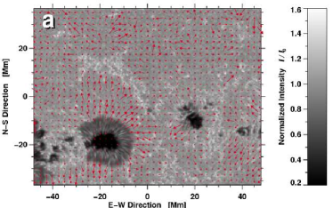
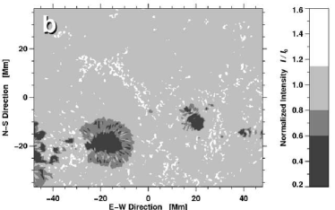
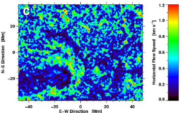
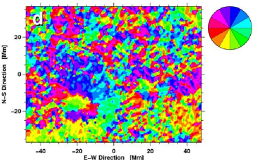
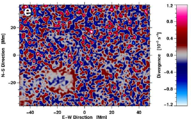
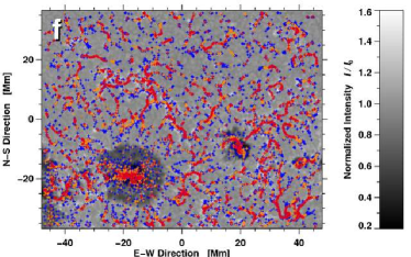
Figure 2: (a) The average (60-minute) G-band image after correction of geometrical foreshortening corresponding to the G-band image shown in Fig. 1a. The red arrows indicate magnitude and direction of the horizontal proper motions. Arrows with a length corresponding to the grid size indicate velocities of 1 km s^-1. (b) Adaptive and fixed intensity thresholds are used to identify conglomerates of G-band bright points, granulation, penumbrae, umbrae, and pores. Color codes are used to point out (c) flow speed and (d) direction in high-resolution flow maps. The flow direction is encoded according to the 12 colors of the compass rose. Sources and sinks in a flow field can be identified in (e) a divergence map. The (f) forward cork maps provides further means of visualizing converging motions. Test particles are displayed after they have followed the flows for 2 (blue), 4 (orange), and 8 h (red). The conspicuous network of corks is related to the spatial scales of the meso-and supergranulation.

Apart from the conventional way of displaying velocity vectors as arrows we present two-dimensional high-resolution speed (Fig. 2c) and azimuth (Fig. 2d) maps. In these maps, the physical quantities are computed for each individual pixel so that the fine structure of the flow field becomes accessible. The color scale for the speed values is the same for all plots in this study. Indeed, we used the same color scale for all flow maps in the database so that flows for different scenes on the Sun can be directly compared. In the azimuth map the direction is encoded in a 12-color compass-rose, which can be found to the very right of this panel. In principle more colors could be used to illustrate the flow direction. However, such plots would become very crowded and are very hard to interpret. The essential features of the flow field, i.e., inward motion of the penumbral grains in the inner penumbra and outward motions related to Evershed and moat flows, can easily be identified.

Divergence (Fig. 2e) and vorticity maps were also compiled for each time-series. The maximum values for divergence ($1.5\times 10^{-3}$ s^-1) and vorticity ($0.6\times 10^{-3}$ s^-1) in these maps are an order of magnitude higher than values found for quiet Sun granulation in previous studies. However, higher values are not surprising, since we calculated them for each pixel in the high-resolution maps capturing more of the small-scale motions. Reassuringly, our values of the $10^{\mathrm{th}}$ percentile for divergence ($4.3\times 10^{-4}$ s^-1) and vorticity ($1.9\times 10^{-4}$ s^-1) are essentially the same as reported by Simon et al. (1994). On the other hand, in the present study the divergence is four times and the vorticity is two times higher than the values presented by Strous et al. (1996) but these values were computed in the proximity of an emerging active region. In summary and keeping in mind the different LCT parameters used in the different studies, the statistical properties of the flow fields as presented in this study are in agreement with previous investigations.

In order to visualize the temporal evolution of the horizontal proper motions, we computed forward (Fig. 2f) and inverse cork maps. Evenly spread test particles are allowed to float forward in time with a given horizontal speed for a certain time interval (see Molowny-Horas, 1994). In the inverse cork map the particles float backward in time. This is accomplished by simply reversing the sign of the velocity components. The forward cork map is used to visualize regions of converging flows and the inverse map is a good tool to study divergence regions. We tracked test particles for consecutively two, four, and eight hours. These particles were initially distributed on an equidistantly spaced grid with a spacing of 10 pixels, i.e., one particle was placed every 0.8 Mm. The most conspicuous feature of the forward cork map are the tracer particles outlining the network of G-band bright points, which corresponds to the supergranular boundaries.

We prepared overview web pages for the respective dates, when suitable time-series of G-band images were available, which contain all the six plots of Fig. 2 along with vorticity and inverse cork maps. The results of this study will ultimately be published as a small GAVO project as a value-added product of the Hinode database.

3.5 Timing issues related to the image capture

LCT delivers localized displacements observed in image pairs. These displacements in conjunction with the time, which has elapsed between the acquisition of both images, yield localized velocity vectors. Therefore, accurate knowledge of the time interval between consecutive images used in the LCT algorithm is essential. The time interval $\Delta t$ for the high-cadence image sequence observed on 2007 June 4 has a bimodal distribution with values $\Delta t$ of 14.4 s (60.7%) and 16 s (39.3%). The average value is $\Delta\bar{t}\approx 15.0$ s. The difference of 1.6 s is an artifact of the polarization modulation. The polarization modulation unit (PMU) is located just behind the telescope exit slit within the optical telescope assembly but before the tip-tilt mirror employed by the correlation tracker (see Tsuneta et al., 2008). A common CCD camera is assigned to both the broad- and narrowband filter imagers (BFI and NFI). The critical timing between camera and PMU is handled by the focal plane package. The PMU is a continuously rotating waveplate, which is always turned on – even for non-polarimetric data such as G-band images. Its rotation period is $T=1.6$ s and all exposure timing is controlled with the clock of the PMU. This is the reason for the non-uniformity in the observed time-interval $\Delta t$.

However, we do not find a bimodal pattern in the LCT displacements but only fluctuations related to evolving features on the Sun and some residual numerical effects. Therefore, we opted to use the fixed time interval $\Delta\bar{t}$ in the data analysis. Sometimes a ‘traffic jam’ in the data transfer might result in even largertiming errors. On the other hand, averaging individual LCT maps over an hour (or longer) will only result in velocity errors of less than a tenth of a precent, i.e., the speed measured by the LCT algorithm is not significantly affected. In summary, accurate timing has to be ensured to obtain reliable LCT flow maps and all data were checked for consistency between recorded time stamps and measured horizontal displacements. Since the individual flow maps during the first and last two minutes of the one-hour sequences do not reflect the true proper motions but are artifacts of the subsonic filtering, we excluded them from the calculation of the average flow maps.

4 Results

4.1 Statistical properties of flow maps and time cadence selection

The one-hour time-series on 2007 June 4 contains 238 G-band images, i.e., the time cadence is $\approx 15$ s. This higher temporal resolution allows us to study the intrinsic accuracy of the LCT algorithm. We calculated LCT maps using seven different time intervals $\Delta t=$ 15, 30, 60, 90, 120, 240, and 480 s. Note that the time interval over which flow maps are averaged is reduced to $\Delta T=3600\leavevmode\nobreak\ \mathrm{s}-\Delta t$, i.e., in case of the longest time cadence by as much as 8 min. However, these slightly different averaging times will not change the results discussed below. When using all individual LCT maps to compute the average horizontal proper motion we refer to such data as the entire sequence. On the other hand, when we split the entire sequence into four disjunct sets, we refer to them as interleaved data sets, i.e., every fourth LCT map is employed to compute the average horizontal proper motion. Since these flow maps cover exactly the same period of time, differences can be directly attributed to the numerical accuracy of the LCT algorithm.

For the entire sequence and interleaved data sets we computed statistical parameters describing the distribution of horizontal proper motions for granulation in the vicinity of active region NOAA 10960. We used the adaptive thresholding algorithm (Eqn. 4) to select only granulation excluding G-band bright points. The proper motions, thus, refer to plasma motions in the absence of any strong magnetic field concentrations. Such selection facilitates comparing horizontal flow speeds and their distributions in all the cases of the present work.

We calculated the mean $\bar{v}$, median $v_{\mathrm{med}}$, maximum $v_{\mathrm{max}}$, and $10^{\mathrm{th}}$ percentile $v_{10}$ of the horizontal flow speeds. Since the maximum speed $v_{\mathrm{max}}$ is only based on a single value, it is easily influenced by numerical errors and the data calibration. The $10^{\mathrm{th}}$ percentile $v_{10}$ is more robust because it describes a property of the entire distribution, i.e., the high velocity tail. Along with these quantities we also calculated the variance $\sigma^{2}_{v}$, standard deviation $\sigma_{v}$, skewness $\gamma_{1,v}$, and kurtosis $\gamma_{2,v}$. The last two statistical parameters describe the deviation of the distribution from a normal distribution.

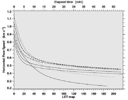
Figure 3: Mean horizontal flow speed as a function of averaged LCT maps for time cadences $\Delta t$ of 15 s (thick dashed), 30 s (thick dash-dotted curve), 60 s (thick dash-triple-dotted curve), 90 s (thick long dashed curve), 120 s (thin dashed), 240 s (thin dotted), and 480 s (thin solid).

We find an increase of the average velocity with increasing time cadence $\Delta t$ starting from about 0.40 km s^-1 for $\Delta t=15$ s, arriving at a maximum value of about 0.47 km s^-1 for $\Delta t=$ 60–90 s, and then decreasing from about 0.45 km s^-1 for $\Delta t=120$ s to 0.34 km s^-1 for $\Delta t=240$ s reaching the lowest value of about 0.23 km s^-1 for $\Delta t=480$ s. Other statistical parameters such as $v_{\mathrm{med}}$, $v_{10}$, $v_{\mathrm{max}}$, $\sigma^{2}_{v}$, and $\sigma_{v}$ follow the same trend.

The initially increasing values can be explained by the time required for a solar feature to move from one to the next pixel. Three velocity values have to be considered: (1) the photospheric sound speed of $\approx$8 km s^-1, (2) the maximum photospheric velocity of $\approx$2 km s^-1 measured by LCT techniques, and (3) the average speed for the proper motion of the granulation of $\approx$0.5 km s^-1. For $\Delta t=15$ s the average displacement is around one tenth of a pixel, whereas the numerical accuracy for a single measurement is only one fifth of a pixel, because the maximum of the cross-correlation function can only be determined with this precision. Thus, in this case a solar feature has not sufficient time to move, which results in underestimating its velocity.

In case of $\Delta t=$ 60–90 s, the horizontal displacement is sufficiently large so that a feature could have moved to one of the neighboring pixels. The speed in individual LCT maps is now well within the range, where numerical accuracy issues are negligible. Starting at $\Delta t=120$ s the mean velocity becomes lower, while there is sufficient time for a solar feature to move quite some distance, the feature might have evolved too much, so that the LCT algorithm might not any longer trace the same feature. This leads to diminished horizontal velocities.

Thus, 60–90 s is the good choice for measuring of horizontal flow speeds with LCT techniques. In this range of the time cadence, the mean values $\bar{v}$ of the interleaved data sets are essentially the same. Their deviations are much smaller than the previously discussed systematic trends. In summary, all flow maps for the database were calculated using $\Delta t=$ 60–90 s. If the time interval $\Delta t$ was shorter, a multiple of the time interval $\Delta t^{\prime}=n\Delta t$ with $n=2,3,$ or 4 was used.

4.2 Determining the duration of the time averages

How many individual LCT maps have to be averaged to yield a reliable flow map? As previously discussed, the parabola fit to the maximum of the cross-correlation sets one limitation. However, there are also method-independent issues to be considered. Solar features evolve over time so that a global pattern reveals itself only after averaging many individual LCT maps. We computed the mean horizontal flow speed as a function of the number of individual LCT maps that were used to arrive at an average flow map. The number of flow maps corresponds to the time interval $\Delta T$ over which the individual flow maps were averaged.

Figure 3 presents this functional dependence for the time cadences from $\Delta t=15$ s to 480 s. All curves start with high velocities when only a few individual LCT maps are averaged. It takes about 20 min before the curves level out and approach an asymptotic value indicating that these average flow maps are still dominated by the motions of fine structure contained within the sampling window. As discusses in the context of the statistical properties of the flow maps, short time cadences $\Delta t$ tend to underestimate the flow speed. If flow speeds have be computed for time intervals shorter than 20 min, in particular for small-scale features, feature tracking methods are more appropriate than LCT techniques.

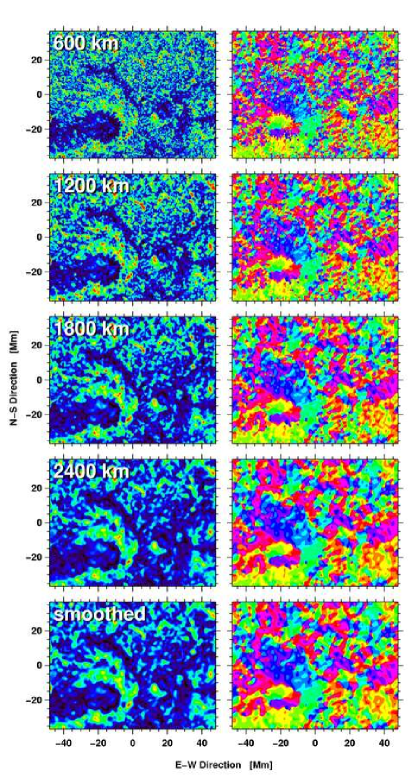
Figure 4: Horizontal flow speed (left ) and azimuth maps (right ) measured using Gaussian kernels with $64\times 64$ pixels and various FWHM. The FWHM of 7.5, 15, 22.5, and 30 pixels correspond to 600, 1200, 1800, and 2400 km on the solar surface, respectively. The bottom row depicts smoothed versions of the $\mathrm{FWHM}=1200$ km speed and azimuth maps. The color coding is the same as in Fig. 2.

We find that all curves up to $\Delta t=90$ s are stacked on top of each other without crossing the next higher curve at any point. Starting at $\Delta t=120$ s we find that the curves corresponding to the longer time cadences cross the other curves after about 20–25 min. This is another indication that solar features have evolved too much so that LCT fails to properly track their motion. This behavior provides an explanation for the spread of velocity values found in literature. In particular, short time-series, as often encountered in ground-based observations, might be biased towards higher velocities. In summary, our choice of 60-minute averages for LCT maps is a conservative one giving solar features sufficient time to reveal the global flow pattern.

4.3 Selection of the sampling window

How do the horizontal proper motions depend on size and FWHM of the Gaussian kernel used in the LCT algorithm? To answer this question, we calculated horizontal proper motions using a Gaussian kernel with $64\times 64$ pixels, which is equivalent to 5120 km $\times$ 5120 km on the solar surface. This larger kernel was chosen to encompass successively broader FWHM. We choose four FWHM of 7.5, 15, 22.5, and 30 pixels corresponding to 600, 1200, 1800, and 2400 km, respectively. The FWHM of 1200 km matches the size of a granule. Individual LCT maps are produced from image pairs separated by 60 s in time. We computed the statistical parameters relating to granulation for the entire sequence and the interleaved data sets. All statistical parameters are decreasing with increasing FWHM. For $\mathrm{FWHM}=600$ km the mean velocity is $\bar{v}=0.48$ km s^-1, which decreases to $\bar{v}=0.47$ km s^-1 for $\mathrm{FWHM}=1200$ km, $\bar{v}=0.41$ km s^-1 for $\mathrm{FWHM}=1800$ km, and further to $\bar{v}=0.37$ km s^-1 for $\mathrm{FWHM}=2400$ km. Small-scale features, which exhibited the highest proper motions, are lumped together with regions of low flow speeds when the FWHM increases. This effect is displayed in Fig. 4, which shows the speed and azimuth maps for the four FWHM. As before, for a given FWHM all statistical parameters agree with each other for up to three significant digits, i.e., there is no indication that the algorithm’s numerical accuracy depends on the FWHM of the kernel used in LCT.

In the case of $\mathrm{FWHM}=1200$ km, the statistical parameters are very close to the ones calculated for the same FWHM but with a kernel of $32\times 32$ pixels. This is not surprising, since the Gaussian kernel assigns a much stronger weight to features in the center of the subimage, i.e., the periphery in the $64\times 64$ pixels FOV has only a small influence in determining the displacement vector for a pair of subimages. This of course only holds true as long as the wings of the Gaussian do not significantly extend beyond the edges of the kernel. Convolving the average flow map ($\mathrm{FWHM}=1200$ km) with a Gausssian kernel, which had a size of $32\times 32$ pixels and $\mathrm{FWHM}=26.4$ pixels (2112 km), we arrive at a smoothed version (see bottom row in Fig. 4), which is virtually identical to the flow map with $\mathrm{FWHM}=2400$ km.

In conclusion, it makes no difference, if one uses a larger FWHM while computing LCT maps or one smoothes the maps after computation. In both cases, the results are virtually the same. Since only minor changes in the LCT results were observed for kernels with $32\times 32$ pixels as compared to $64\times 64$ pixels, the smaller kernel was chosen significantly reducing the computing time. Furthermore, the smallest FWHM produces the most detailed flow maps. However, we chose a FWHM of 1200 km favoring the spatial scales of granulation, which covers the largest fraction of the observed area. Additional smoothing can still be applied in the later data analysis stages to either reduce noise or to track flows on larger spatial scales. For case studies of sunspots fine structure smaller FWHM might be more appropriate.

4.4 Numerical errors in calculating flow maps

We computed the pixel-to-pixel rms-error for the magnitude and direction of the flow velocity using the interleaved data sets for different time cadences $\Delta t$ and for different FWHM of the sampling window. Six difference maps (sets $1-2$, $1-3$, $1-4$, $2-3$, $2-4$, and $3-4$) can be computed from the four interleaved data sets, thus for each pixel we can derive the errors, which are primarily due to numerical errors inherent to the LCT algorithm. In case of different time cadences, the rms-error in velocity is 15–90 m s^-1 from shortest to longest cadence. The corresponding rms-error in direction is $5^{\circ}$–$30^{\circ}$. However, for cadences in the range of 60–90 s, which is the range used to create the database, the rms-error of the velocity is typically in the range from 35–70 m s^-1, while the values for the direction vary by as much as $10^{\circ}$–$15^{\circ}$. The largest variations in direction are observed near the boundaries of patches showing coherent flows. Even after correcting the $2\pi$ ambiguity in the difference maps, we find high values at these locations. As a side note, the rms-error in direction justifies our choice of a color wheel with only twelve segments in the display of the azimuth maps. One segment covers $30^{\circ}$ so that pixel-to-pixel variations of about $\pm 15^{\circ}$ are suppressed. Otherwise, the azimuth maps would appear too crowded distracting from the overall flow pattern.

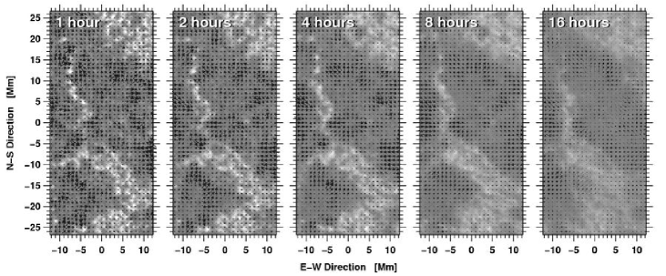
Figure 5: Time-averaged G-band images with horizontal flow vectors computed for $\Delta T=$ 1, 2, 4, 8, and 16 h. Arrows with a length corresponding to the grid spacing indicate velocities of 1 km s^-1. The background images are displayed in the intensity range $0.5\leq I/I_{0}\leq 1.5$.

In the case of different FWHM of the sampling window, rms-errors for speed and direction decrease with increasing FWHM. The velocity error is 35 m s^-1 and the error in direction is about $10^{\circ}$ for a FWHM of 1200 km. These errors decreases to 15 m s^-1 and $5^{\circ}$ for a FWHM = 1800 km and further to 10 m s^-1 and $4^{\circ}$ for a FWHM = 2400 km. Here, the decreasing rms-errors can be attributed to the smoothing effect of a wider sampling window, i.e., more pixels are used with higher weights in the cross-correlation. Furthermore, the rms-error in magnitude and direction for the time cadence $\Delta t=60$ s is nearly the same regardless of the size of the Gaussian kernel ($32\times 32$ pixels vs. $64\times 64$ pixels.

Finally, we calculated Pearson’s correlation coefficient between LCT maps of the interleaved data sets. Pearson’s correlation coefficient indicates the degree of a linear relationship between two variables. A positive value of unity indicates that the data sets are identical disregarding a linear scaling factor. The linear correlation coefficient for different time cadences $\Delta t$ decreases from 0.99 to 0.93 starting at the shortest and ending at the longest cadence. The high degree of correlation indicates that all essential features of the flow field are capture by the LCT algorithm. The monotonic decrease, however, indicates that numerical errors increase when the cadences $\Delta t$ become too large.

4.5 Long-lived features in flow maps

The one-hour time interval over which the LCT maps are averaged is not sufficient to identify features, which need longer to evolve such as meso- and supergranulation. Therefore, to clearly identify the boundaries of these large-scale convective cells and to visualize the effects of longer time averages, we averaged LCT maps over $\Delta T=$ 1, 2, 4, 8, and 16 h utilizing the long-duration data set with 960 images and a time cadence $\Delta t=60$ s.

As before, we calculated the statistical parameters for the entire sequence and the interleaved data sets for granulation. All velocity values decrease with increasing time intervals over which, the individual LCT maps are averaged. For $\Delta T=1$ h the mean velocity is $\bar{v}=0.44$ km s^-1, which decreases to $\bar{v}=0.38$ km s^-1 for $\Delta T=2$ h, $\bar{v}=0.34$ km s^-1 for $\Delta T=4$ h, $\bar{v}=0.30$ km s^-1 for $\Delta T=8$ h, and further to $\bar{v}=0.23$ km s^-1 for $\Delta T=16$ h. The mean speed approaches a value for the global flow field with increasing $\Delta T$. However, the value for $\Delta T=1$ h is only slightly smaller than previously computed for the high-cadence sequence. Such small deviations ($<0.05$ km s^-1) reflect only minute differences between the scenes on the solar surface.

Table 1: Parameters describing the horizontal proper motions of granulation and G-band bright points calculated over $\Delta T=1,2,4,8,\mathrm{and}$ 16 h.

	Granulation						Bright points
$\Delta T$	$\bar{v}$	$v_{\mathrm{med}}$	$v_{10}$	$v_{\mathrm{max}}$	$\sigma_{v}$		$\bar{v}$	$v_{\mathrm{med}}$	$v_{10}$	$v_{\mathrm{max}}$	$\sigma_{v}$
[h]	[km s-1]	[km s-1]	[km s-1]	[km2 s-2]	[km s-1]		[km s-1]	[km s-1]	[km s-1]	[km2 s-2]	[km s-1]
1	$0.43$	$0.39$	$0.78$	$1.86$	$0.24$		$0.22$	$0.22$	$0.37$	$0.70$	$0.10$
2	$0.39$	$0.36$	$0.69$	$1.42$	$0.21$		$0.22$	$0.22$	$0.35$	$0.55$	$0.10$
4	$0.34$	$0.31$	$0.60$	$1.25$	$0.19$		$0.17$	$0.17$	$0.27$	$0.52$	$0.08$
8	$0.30$	$0.29$	$0.50$	$0.87$	$0.15$		$0.15$	$0.15$	$0.24$	$0.45$	$0.07$
16	$0.23$	$0.22$	$0.38$	$0.74$	$0.12$		$0.12$	$0.12$	$0.20$	$0.41$	$0.06$

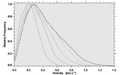
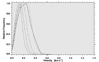
Figure 6: Relative frequency distributions of horizontal proper motions for quiet Sun (left ) and G-band bright points (right ) calculated over $\Delta T=1$ h (solid curve), 2 h (dotted curve), 4 h (dashed curve), 8 h (dash-dot-dotted curve), and 16 h (dash-triple dotted curve)

Fig. 5 contains the time-averaged G-band images with superposed arrows indicating speed and direction of the horizontal proper motions for $\Delta T=1$, 2, 4, 8, and 16 h. The region shows granulation and G-band bright points to the west of active region NOAA 11930. Magnetic features dominate the long-duration time averages, i.e., the flow speed is low where strong magnetic fields are present in the chromospheric network and conversely the speed is high where G-band bright points outline the boundaries of large-scale convective cells. The high speeds associated with the local convective pattern of granules have diminished for the long-duration flow maps and only the converging motion towards the cell boundaries remains explaining the statistical properties of the velocity values discussed above. The overall visual impression of the vector maps is that the arrows are more ordered in the long-duration maps, whereas in the short-duration maps ($\Delta T=1$ and 2 h) a larger scatter of the flow vectors is observed on smaller scales. Nonetheless, the imprint of the the meso- and/or supergranulation is already visible in the short-duration flow maps and becomes more prominent the longer the time interval over which the LCT maps are averaged. Strong converging motions can be found in Fig. 5 near the vertical alignment of G-band bright points in the north-east corner of the FOV and at the boundary of the larger supergranular cell in the south-east corner of the FOV. The supergranule also contains substructure on smaller scales, i.e., a strong divergence center exactly in the central FOV, which can be clearly seen after averaging for at least $\Delta T=2$ h.

We plotted relative frequency distributions of flow fields spanning time intervals of $\Delta T=$ 1, 2, 4, 8, and 16 h in Fig. 6 to gain insight into the statistical properties of the long-duration data sets – this time both for granulation and for G-band bright points. The statistical parameters characterizing these distributions are provided in Tab. 1 for reference. The distribution describing granulation for the shortest time interval ($\Delta T=1$ h) is the broadest and has an extended high velocity tail. Interestingly, for velocities up to 0.6 km s^-1 this distribution is virtually the same as the distribution for an averaging time, which is twice as long ($\Delta T=2$ h). The only difference is the high velocity tail. This indicates that proper motions on small scales still make their presence known, if individual LCT maps are not averaged for at least two hours. The longer $\Delta T$, the more are the peaks of these distributions shifted towards lower velocity values (from 0.43 to 0.23 km s^-1) and their standard deviations are progressively becoming smaller (from 0.24 to 0.12 km s^-1). The progression of the frequency distributions shown in the left panel of Fig. 6 supports the conclusion that the essential features of long-duration LCT maps have been captured for $\Delta T=$ 8–16 h.

The frequency distributions for G-band bright point differ in some aspects from those for granulation. The high velocity tail is less prominent and all statistical parameters describing the distributions are reduced by about a factor of two. The two distribution with the shortest time intervals ($\Delta T=1$ and 2 h) show a hint of a bimodal distribution, and they are skewed towards higher velocity values. However, this might be an artifact of the adaptive thresholding algorithm, since the areas covered by G-band bright points are smaller and well defined in the short-duration intensity maps. Thus, considering the FWHM = 1200 km of the sampling window, a larger contribution from granulation is expected, if more isolated G-band bright points are present in the maps, which are used for threshholding. It should be noted that Eqn. 4 was slightly modified to accommodate the longer time intervals, which leads to a fuzzier appearance of the area covered by G-band bright points and results in a diminished contrast of the G-band bright points. Since no contemporary magnetograms with comparable spatial resolution were available, we cannot comment on the influence of flux emergence or dispersal during the observed time interval. However, active region NOAA 10930 showed pronounced activity. In particular, the penumbra of the small sunspot just to the east of the FOV decayed and resulted in continuous flaring in the active region.

Even though long-duration time averages are an important tool when studying large-scale convective patterns or the persistent motions in an active region, the scarcity of such data sets argues against their use for comprehensive and comparative studies. Since most of the characteristics of flow fields are already captured in one-hour averages, we opted for $\Delta T=1$ h. Furthermore, selecting $\Delta T=1$ h allows us to study changes in long-duration time-series by computing averaged flow maps every 30 min. Another consideration is that one hour is more then ten times the typical lifetime of granules so that the proper motions of individual granules should be negligible and global motion patterns will reveal themselves.

Table 2: Statistical parameters describing the frequency distributions of the horizontal proper motions of various solar features.

	$\bar{v}$	$v_{\mathrm{med}}$	$v_{10}$	$v_{\mathrm{max}}$	$\sigma^{2}_{v}$	$\sigma_{v}$	$\gamma_{1,v}$	$\gamma_{2,v}$
Feature	[km s-1]	[km s-1]	[km s-1]	[km s-1]	[km2 s-2]	[km s-1]
All	$0.44$	$0.40$	$0.83$	$1.95$	$0.07$	$0.27$	$0.76$	0$0.21$
Granulation	$0.47$	$0.43$	$0.85$	$1.95$	$0.07$	$0.27$	$0.67$	0$0.08$
Penumbra	$0.30$	$0.24$	$0.62$	$1.43$	$0.05$	$0.23$	$1.46$	0$2.07$
Umbra	$0.23$	$0.19$	$0.40$	$1.92$	$0.04$	$0.20$	$3.66$	$20.44$
Bright points	$0.23$	$0.20$	$0.43$	$1.21$	$0.03$	$0.15$	$1.43$	0$2.65$

4.6 Frequency distributions for different solar features

The simplest approach to describe flow fields would be to compute the overall frequency distributions for a particular FOV. However, this simplistic approach is insufficient to recover the underlying physics of plasma motions in the presence (or absence) of strong magnetic field. We used the adaptive thresholding algorithm (Eqn. 4) described in Sect. 3.4 to compute frequency distributions for granulation, penumbrae, umbrae/pores, G-band bright points, and the entire FOV regardless of the features contained in this region. For this case study, we used the high-cadence sequence (see Fig. 2b for the thresholded image) with $\Delta t=60$ s, $\Delta T=1$ h, and a FWHM = 1200 km. The respective distributions are shown in Fig. 7 and the corresponding statistical parameters are summarized in Tab. 2. Similar plots and tables will be included in the database subsuming the more than 200 data sets, which have been analyzed as part of this study. We provide Fig. 7 and Tab. 2 to facilitate comparison with other case studies. However, these data are not representative (in the sense of a mean value) for all data sets contained in the database.

A barely detectable shoulder in the frequency distribution for the entire FOV and the extended high velocity tail hint already that this distribution contains contributions from various solar features. Its mean velocity $\bar{v}=0.44$ km s^-1 is slightly smaller than the corresponding value for granulation $\bar{v}=0.47$ km s^-1, which dominates the FOV. The distribution for granulation is broader and a low value of kurtosis ($\gamma_{2,v}=0.08$) leads to a flatter peak, where any indication of a shoulder is absent. There is a noticeable difference in the distributions of strong magnetic elements and granulation. The distributions for G-band bright points, umbral and penumbral regions are narrow, have sharp peaks, and are shifted towards lower velocities. The mean velocity for these regions varies from $\bar{v}=0.30$ km s^-1 for penumbrae to $\bar{v}=0.23$ km s^-1 for umbrae/pores and G-band bright points. Interestingly, the distributions for umbrae/pores and G-band bright point are virtually identical, while that for penumbra has significant contributions at velocities above 0.4 km s^-1. This is indicative of the more complex flow fields in penumbrae, where penumbral grains move preferentially in the radial direction – inward in the inner penumbra and outward in the outer penumbra. This also illustrates that some of the small-scale horizontal proper motions can be capture with the current implementation of the LCT algorithm.

4.7 Flow maps for different spatial resolution

Finally, we would like to address the question on how the spatial resolution affects the determination of the horizontal proper motions. We used the high-spatial resolution sequence of Sect. 2.3 and treated it exactly the same as all the other data with the exception that the G-band images were sampled at 40, 80, 120, 160, and 200 km after correction of geometrical foreshortening. Multiple of 40 km were chosen to match the Hinode SOT/BFI pixel size of 0.055″. Obviously the number of pixels in the sampling window had to be adjusted. However, shape, size, and FWHM = 1200 km of the sampling window were not changed.

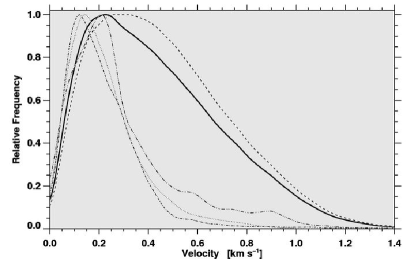
Figure 7: Relative frequency distributions of horizontal proper motions computed for all solar features (solid curve), G-band bright points (dotted curve), granulation (dashed curve), umbra (dash-dotted curve) and penumbra (dash-dot-dotted curve).

The values describing the respective frequency distributions are given in Tab. 3. They were computed for areas with granulation covering the full FOV. However, to visualize the minute changes in the flow maps, we show in Fig. 8 only an area of 8 Mm $\times$ 8 Mm. In the top row of Fig. 8 flow vectors are superposed on one-hour average G-band images with different image scales. This scene on the Sun is dominated by converging motions towards the X-shaped alignment of G-band bright points. The grid spacing corresponds to 320 km and the length of the arrows was chosen so that an arrow with a length of exactly the grid spacing corresponds to 0.5 km s^-1. The difference are so minute that they only show up in difference images of the LCT maps. The bottom row of Fig. 8 shows the flow speed for each pixel in the FOV at the same color scale as used in all the other figures. The overall appearance to the flow field is the same. However, the low resolution maps look blockier due to the coarser sampling and some of the fine structure starts to fade out.

Table 3: Statistical parameters describing the frequency distributions of the horizontal proper motions for various image scales.

Image scale $\alpha$		$\bar{v}$	$v_{\mathrm{med}}$	$v_{10}$	$v_{\mathrm{max}}$	$\sigma^{2}_{v}$	$\sigma_{v}$	$\gamma_{1,v}$	$\gamma_{2,v}$
[pixel-1]	[km pixel-1]	[km s-1]	[km s-1]	[km s-1]	[km s-1]	[km2 s-2]	[km s-1]
0.055″	040	0.54	0.52	0.89	1.60	0.07	0.26	0.42	$-0.09$
0.110″	080	0.53	0.52	0.88	1.62	0.07	0.26	0.42	$-0.09$
0.165″	120	0.52	0.51	0.87	1.58	0.07	0.26	0.46	$-0.04$
0.220″	160	0.50	0.48	0.83	1.54	0.06	0.25	0.50	$\phantom{0}0.05$
0.275″	200	0.47	0.45	0.79	1.57	0.06	0.24	0.55	$\phantom{0}0.19$

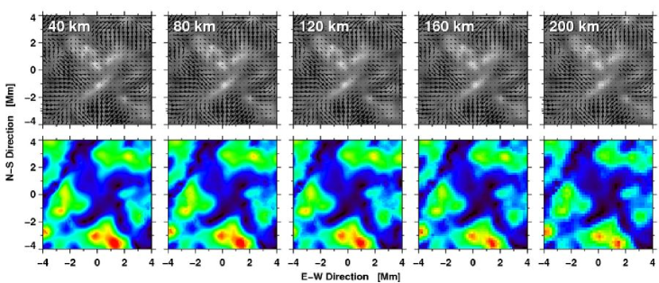
Figure 8: Time averaged G-band images with horizontal flow vectors (top ) and flow speed maps (bottom ) for different spatial resolution. Arrows with the length corresponding to the grid spacing indicate velocities of 0.5 km s^-1.

In summary, the average velocity diminishes from 0.54 km s^-1 at the highest spatial resolution to 0.47 km s^-1 at the lowest resolution. This trend is the same for all other parameter with the exception of kurtosis and skewness, which show some (negligible) scatter. Changes of less than 15% in velocity cannot explain the broad range of velocity values for horizontal proper motion reported in literature. Note, however, that Hinode data is not susceptible to the adverse affect of seeing, i.e., ground-based LCT measurements will be much more affected depending on the spatial resolution. Even though seeing should not introduce a systematic bias in LCT (see November & Simon, 1988), it will still affect the noise in the LCT measurements.

5 Conclusions

Many case studies exist in the literature describing horizontal proper motions based on LCT or FT techniques. Even though most of them agree on the morphology of the observed flows, significant differences are found when quantifying the flow properties. Besides obvious differences inherent to the techniques, the choice of parameters such as sampling window, time cadence, and duration can significantly impact the outcome. Some results of previous studies are provided in Tab. 4 for convenience and to ease comparison with the present investigation.

We have presented the implementation of an LCT algorithm, which was used to create a database of flow maps derived from time-series of G-band images observed with Hinode/SOT. The parameter study and error analysis will also be beneficial to other studies using LCT techniques. Even for observations from the ground our results provide guidance, since LCT techniques are not biased by seeing (see November & Simon, 1988) so that our error estimates can be understood as a lower limit.

Justifying the choice of parameters for LCT and FT algorithms is always a challenging task, which should be driven by the scientific purpose of the study. In the present study, the emphasis was on creating a database of flow maps, which can be used in statistical investigations regardless of the type of solar feature, location on the Sun, or solar activity. In the following list, we summarize our choice of LCT parameters.

Table 4: Summary of LCT results in previous studies.

$\alpha$	FWHM	$d_{\mathrm{grid}}$	$\Delta t$	$\Delta T$	$\bar{v}\pm\sigma_{v}$	$v_{\mathrm{med}}$	$v_{\mathrm{max}}$	Remarks
[pixel-1]			[s]	[min]	[km s-1]	[km s-1]	[km s-1]
November & Simon (1988) and November (1989)								continuum images at $\lambda 517.5$ nm, Universal Birefringent Filter (UBF), 12 s exposure time, Dunn Solar Telescope/Sacramento Peak
0.250″	3.3″	2.0″	67	80	0.5–1.0 (for source regions)
Brandt et al. (1988)								broad-band (5.4 nm) images at $\lambda 469.6$ nm, Solar Optical Universal Polarimeter (SOUP), 20 ms exposure time, Swedish Solar Vacuum Telescope/Observatorio del Roque de los Muchachos
0.035″	2.4″	0.8″	60	79	0.67		01.2
Title et al. (1989)								broad-band (100 nm) images at $\lambda 600$ nm, SOUP, short-exposure images recorded on photographic film, Spacelab 2, provides also proper motion measurements for other FWHM down to 1.0″
0.161″	4.0″	2.5″	60	28	0.37$\pm 0.45$		$<$1.2
Berger et al. (1998)								G-band images $\lambda 430.5\pm 0.6$ nm, SOUP, 20 ms exposure time, SVST, LCT parameter study and comparison of proper motions between granulation and network
0.083″	0.83″	0.4″	24	70	$1.10\pm 1.30$	0.70	$\sim$4.0
Shine et al. (2000)								continuum images near the Ni i $\lambda$676.8 nm line, Michelson Doppler Imager (MDI), Solar Heliospheric Observatory (SoHO), long-duration sequence of 45.5 h
0.600″	4.8″	2.4″	60	60	0.49	0.47	01.5

• $\alpha$: image scale, FWHM: width of the sampling window, $d_{\mathrm{grid}}$: grid spacing on which LCT flow vectors are computed, $\Delta t$: image cadence, $\Delta T$: time interval over which individual LCT maps are averaged, $\bar{v}\pm\sigma_{v}$: average flow speed and standard deviation, $v_{\mathrm{med}}$: median value of the frequency distribution, and $v_{\mathrm{max}}$: highest observed flow speed.

• The flow maps are based on time-series of G-band images with cadences $\Delta t$ between 60 s and 90 s. If the cadence is shorter, features with low velocities cannot be accurately tracked, whereas in longer cadences features will have evolved too much so that the algorithm might not recognize them any longer. Our cadence selection is conservative in the sense that we limit our database in favor of better comparability. Note that there is a significant number of G-band time-series with cadences of about 2 min, which are not included in our database.

• The evolution of individual features (granules, bright points, penumbral grains, umbral dots, etc.) dominate flow fields on short time scales. Therefore, averaging over time scales significantly longer than the lifetime of the aforementioned features is necessary to yield the global flow field. Our choice of $\Delta T=1$ h over which the flow maps are averaged ensures that the global flow fields has emerged from the motions of individual features and that sufficient flow maps were averaged to reduce the numerical rms-errors for magnitude and direction of the flow vectors to reasonable values of 35–70 m s^-1 and 10–15^∘, respectively. Note that $\Delta T=1$ h is not an appropriate choice for studies focusing on meso- and supergranulation because the associated flow pattern is still very noisy and could be more easily perceived in longer time averages. However, long-duration time-series are rare to facilitate such studies. Whenever, time-series with longer durations were available, we computed one-hour flow maps with an overlap of 30 min so that the temporal evolution of the flow field can be monitored, which is of particular interest for the investigation of explosive events such as flares, filament eruptions, and coronal mass ejections.

• In principle, the spatial resolution of Hinode/SOT would allow to track features, which are smaller than one second of arc. Our choice of a Gaussian sampling window with 32 $\times$ 32 pixels and a FWHM of 1200 km was again motivated by establishing a database of flow maps for statistical studies. Therefore, we used a FWHM, which corresponds approximately to the size of a granule, which is one of the ‘largest’ elements of solar fine structures. Tracking flows on larger spatial scales can still be accomplished by smoothing the flow maps after the fact.

In forthcoming studies, we will use the database of flow maps to study the statistical properties of pores, the motions in sunspot penumbrae, and their relation to the flow pattern observed in the moat of sunspots. Several years of G-band time-series and more than 1000 individual flow maps facilitate the study of such flows during the life cycle of solar features and environment, i.e., as a function of solar activity or the complexity of the surrounding magnetic field. Once thoroughly tested, the value-added Hinode/SOT data will be made available as a small project within the scope of GAVO.