QUANTUM VORTICES AND TRAJECTORIES
IN PARTICLE DIFFRACTION

Abstract

We investigate the phenomenon of the diffraction of charged particles by thin material targets using the method of the de Broglie-Bohm quantum trajectories. The particle wave function can be modeled as a sum of two terms $\psi=\psi_{ingoing}+\psi_{outgoing}$. A thin separator exists between the domains of prevalence of the ingoing and outgoing wavefunction terms. The structure of the quantum-mechanical currents in the neighborhood of the separator implies the formation of an array of quantum vortices. The flow structure around each vortex displays a characteristic pattern called ‘nodal point - X point complex’. The X point gives rise to stable and unstable manifolds. We find the scaling laws characterizing a nodal point-X point complex by a local perturbation theory around the nodal point. We then analyze the dynamical role of vortices in the emergence of the diffraction pattern. In particular, we demonstrate the abrupt deflections, along the direction of the unstable manifold, of the quantum trajectories approaching an X-point along its stable manifold. Theoretical results are compared to numerical simulations of quantum trajectories. We finally calculate the times of flight of particles following quantum trajectories from the source to detectors placed at various scattering angles $\theta$, and thereby propose an experimental test of the de Broglie - Bohm formalism.

1 Introduction

The aim of the present paper is to implement the method of quantum trajectories, known as de Broglie - Bohm theory De Broglie [1925]; Bohm [1952] in the phenomenon of the diffraction of charged particles by thin material targets. In the de Broglie - Bohm theory we consider trajectories tracing the quantum currents. A trajectory is determined by the initial particle’s position and by the pilot wave equation of motion

$${d\mathbf{r}\over dt}={\hbar\over m}Im({\nabla\psi(\mathbf{r},t)\over\psi(\mathbf{r},t)})$$ (1)

where $\psi$ is the wavefunction (‘pilot wave’), $m$ is the particle mass and $\hbar$ is Planck’s constant. This equation implies Newton’s equation of motion in a potential

$${U(\mathbf{r},t)}=V(\mathbf{r},t)+Q(\mathbf{r},t)$$ (2)

where ${Q(\mathbf{r},t)}$ is the ‘quantum potential’, an extra term caused by the wavefunction $\psi$ :

$${Q(\mathbf{r},t)}=-{\hbar^{2}\over 2m}{\nabla^{2}|\psi|\over|\psi|}.$$ (3)

The probability density of an ensemble of particles guided by the same $\psi$ - field is ${\rho(\mathbf{r},t)}=|\psi(\mathbf{r},t)|^{2}$. The equations of motion (1) imply the continuity equation for $\rho$. Furthermore, in the one-particle case, the Bohmian trajectories are equivalent to the stream lines defined by the quantum probability current $\mathbf{j}=(\hbar/2mi)(\psi^{*}\nabla\psi-\psi\nabla\psi^{*})$. Thus, the Bohmian method yields practically equivalent results to Madelung’s quantum hydrodynamics Madelung [1926].

Bohm’s trajectories have been proved useful in i) constructing efficient numerical schemes for the integration of Schrödinger’s equation via swarms of trajectories (e.g. Wyatt [2005]; Sanz et al. [2002]; Oriols [2007]), and ii) visualizing processes for which no other intuitive picture could be obtained. Examples of the latter are the quantum tunneling effect Lopreore [1999], the (particle) two-slit experimentPhilippidis et al. [1979], ballistic transport through ‘quantum wires’ Beenakker & van Houten [1991], molecular dynamics Gindensperger [2003], dynamics in nonlinear systems with classical focal points or caustics Zhao & Makri [2003] and rotational or atom-surface scattering Sanz et al. [2004]. A final application regards the relation of chaotic quantum motions to the dynamical origin of ‘quantum relaxation’ Vallentini & and Westman [2005]; Efthymiopoulos & and Contopoulos [2006]; Bennett [2010]; Colin & Struyve [2010], namely the justification of the approach (as time increases) of a quantum system to Born’s rule $\rho=|\psi|^{2}$, even if the initial conditions were allowed to deviate from this rule ($\rho_{initial}\neq|\psi_{initial}|^{2}$).

In the case of the diffraction of charged particles, we find some new phenomena due to the structure of quantum currents and to their effects on quantum trajectories. In particular, we find that the quantum flow is always characterized by the formation of an array of quantum vortices delineated along a locus called separator, i.e. a sharp boundary between the domains of prevalence of the ingoing and outgoing flow. The local current structure in a vortex forms a pattern called ‘nodal point - X-point complex’. This has been previously investigated theoretically in Efthymiopoulos et al. [2007]; Contopoulos & Efthymiopoulos [2008]; Efthymiopoulos et al. [2009]. Here we adapt this analysis in the particular problem of particle diffraction, in order to determine the number and location of all critical points of the quantum flow, as well as to determine the size of the nodal point - X-point complexes. The main result of this analysis is that the deflection of quantum trajectories is due to their approaches close to X-points. In fact, the trajectories follow the directions of the asymptotic manifolds of the X-points, and this fact alone suffices to explain the emergence of the whole diffraction pattern.

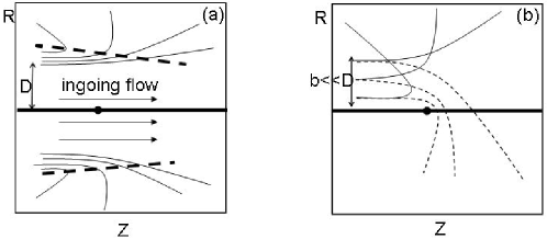
Figure 1: (a) Schematic representation of the quantum trajectories in the scattering or diffraction problem. Deflection takes place for quantum trajectories with initial conditions of an $O(D)$ distance away from the principal beam axis (z-axis). The thick dashed curves illustrate the separator between ingoing and outgoing (from the target) flow. The concentration of the quantum trajectories to various Bragg angles is shown in Figure 5 below. (b) Same as in (a) but in the approximation of classical Rutherford scattering for repelling (—), or attracting ($\cdot\cdot\cdot$) forces.

Passing to a global description of the quantum trajectories, we identify a number of important differences between Bohmian and classical trajectories, which are summarized with the help of a schematic representation (Figure 1). Four main differences are:

a) In the case of quantum trajectories, the scattering angle increases when the impact parameter increases (Fig.1a)(this is explained in section 4), while the opposite is true in the classical case.
b) The deflection of Bohmian trajectories takes place for initial conditions at an $O(D)$ distance from the principal axis of the ingoing beam (z-axis), where $D$ is the transverse quantum coherence length. A typical value for $D$ in electron beams is $D\geq 10^{-6}m$. On the contrary, for classical Rutherford scattering the impact parameter $b$ is many orders of magnitude smaller $(b\sim 10^{-13}m$ ).
c) Bohmian trajectories have the same form in both cases of repelling and attractive forces (Figure 1a), a behavior contrasted to the form of trajectories in the approximation of classical Rutherford scattering (Fig.1b).
d) The most important difference regards the times of flight of particles to detectors placed at different scattering angles $\theta$. The times of flight are shorter for larger impact parameters in the quantum case, independently of the sign of the interacting charges (while the times of flight depend on this sign in the classical case and they are, in general, much shorter than in the quantum case). This effect suggests an interesting experimental test that will be described in section 5.

2 Wave function

We consider a cylindrical beam of particles of mass $m$ and charge $Z_{1}e$ incident on a material target centered at the origin of the coordinate system of reference. Cylindrical coordinates are denoted by $z$ (horizontal), $R$ (transverse) and by the azimuth $\varphi$. Use is also made of spherical coordinates $r=(z^{2}+R^{2})^{1/2}$, $\theta=\tan^{-1}(R/z)$, and $\varphi$.

The quantum-mechanical description of the diffraction process has been discussed extensively (see, for example, Peng et al. [2004]; Peng [2005] for reviews and further references). Here, we adopt a simplified model which is sufficient for all practical purposes in the analysis below. For the interaction of the incident charged particles with any individual atom in the target, we adopt a screened Coulomb potential

$$U(\mathbf{r-r_{j}})={1\over 4\pi\epsilon_{0}}{Z_{1}Ze^{2}\exp(-|\mathbf{r}-\mathbf{r}_{j}|/r_{0})\over|\mathbf{r}-\mathbf{r}_{j}|}$$ (4)

where $Z$ is the nuclear charge, $\mathbf{r}_{j}$ is the position of the $j-th$ atom in the target and $r_{0}$ is a constant representing the screening range, whose value is taken of the order of the atomic size. The total potential felt by one incident particle is the sum of the individual potentials:

$$V(\mathbf{r})=\sum_{j=1}^{N}U(\mathbf{r}-\mathbf{r}_{j})~{}~{}$$ (5)

where $N$ is the total number of atoms effectively participating in the process of diffraction.

In order to describe diffraction quantum-mechanically, we specify a model for the wavefunction $\psi$ of diffracted particles (considering only elastic scattering). To this end, we first find the eigenfunctions $\phi$ of the time-independent Schrödinger equation:

$$-{\hbar^{2}\over 2m}\nabla^{2}\phi+V(\mathbf{r})\phi=E\phi$$ (6)

where $\phi$ is an eigenfunction corresponding to the energy value $E>0$ of an incident particle, and $V(r)$ in (6) is a time-averaged form of (5). We solve Eq.(6) following Born’s approximation method (for $|V|<<E$)and expand $\phi$ as

$$\phi=\phi_{0}+\phi_{1}+\phi_{2}+...$$ (7)

where $\phi_{0}=O(1)$, $\phi_{1}=O(V/E)$, $\phi_{2}=O(V^{2}/E^{2})$ etc. All the essential phenomena appear already when only the two first terms of the expansion $\phi\simeq\phi_{0}+\phi_{1}$ are considered. We then find

$$\phi_{\mathbf{k}}(\mathbf{r})\simeq e^{i\mathbf{k\cdot r}}-{Z_{1}Ze^{2}\over 4\pi\epsilon_{0}}{m\over\hbar^{2}}{e^{ikr}\over r}\left(\sum_{j=1}^{N}e^{i\mathbf{(k-k_{n})\cdot r_{j}}}\right){1\over k^{2}\sin^{2}(\theta/2)+1/r_{0}^{2}}\left[1+O\left({k<r_{j}^{2}>\over r}\right)\right]$$ (8)

where i) the label $\mathbf{k}$ refers to any vector in Fourier space with modulus equal to $k=(2mE)^{1/2}/\hbar$, ii) $\mathbf{k_{n}}=k\mathbf{n}$ with $\mathbf{n}=\mathbf{r}/r$, and iii) $<r_{j}^{2}>=(1/N)\sum_{j=1}^{N}r_{j}^{2}$. The corrections due to the $O(k<r_{j}^{2}>/r)$ and $1/r_{0}^{2}$ terms will be omitted since they do not affect essentially the analysis.

The time-dependent eigenfunctions are now given by $\psi_{\mathbf{k}}(\mathbf{r},t)=\exp(-i\hbar k^{2}t/2m)\phi_{\mathbf{k}}(\mathbf{r})$. The electron wavefunction can be modeled as a superposition of eigenfunctions

$$\psi(\mathbf{r},t)={1\over(2\pi)^{3/2}}\int d^{3}\mathbf{k}~{}\tilde{c}(\mathbf{k})\psi_{\mathbf{k}}(\mathbf{r},t)$$ (9)

where $\tilde{c}(\mathbf{k})$ are Fourier coefficients. Because of the collimation, the ingoing term of the wavefunction at $t=0$ can be modeled as a traveling plane wave along the z-direction times a Gaussian in the transverse direction with dispersion $\sim D$, i.e.

$$\psi_{ingoing}(\mathbf{r},t=0)={1\over\sqrt{2}\pi D}\times\exp\left(-{R^{2}\over 2D^{2}}+i(k_{0}z)\right)~{}~{},$$ (10)

where, assuming that the particles are monoenergetic, the constant $k_{0}$ yields the average momentum $p_{0}=\hbar k_{0}$, or kinetic energy $E_{0}=\hbar^{2}k_{0}^{2}/2m$ along the z-direction. The value of the transverse quantum coherence length $D$, which turns to be a crucial parameter in the analysis below, depends on the details of the electron emission and collimation process.

The Fourier coefficients $\tilde{c}(\mathbf{k})$ for which $\psi_{ingoing}$ has the form (10) are given by:

$$\tilde{c}(\mathbf{k})=\int d^{3}\mathbf{r}~{}\psi_{ingoing}(\mathbf{r},t=0){e^{-i\mathbf{k\cdot r}}\over(2\pi)^{3/2}}={\delta(k_{z}-k_{0})\over\pi^{1/2}\sigma_{\perp}}\exp\left(-{k_{x}^{2}+k_{y}^{2}\over 2\sigma_{\perp}^{2}}\right)$$ (11)

where $\sigma_{\perp}=D^{-1}$. Substituting (11) into (9), and using (8), we can evaluate the form of the wavefunction at all times $t$. After some algebra we find

$$\psi(\mathbf{r},t)=\psi_{ingoing}(\mathbf{r},t)+\psi_{outgoing}(\mathbf{r},t)$$ (12)

where

$$\psi_{ingoing}(\mathbf{r},t)={1\over\sqrt{2}\pi}{D\over{\left(D^{2}+i\hbar t/m\right)^{1/2}}}e^{-{R^{2}\over 2(D^{2}+i\hbar t/m)}+i(k_{0}z-k_{0}^{2}\hbar t/2m)}$$ (13)

$$\psi_{outgoing}(\mathbf{r},t)=-{1\over\sqrt{2}\pi}{D\over{\left(D^{2}+i\hbar t/m\right)^{1/2}}}{Z_{1}Ze^{2}\over 4\pi\epsilon_{0}}{m\over 2\hbar^{2}}{S_{eff}(k_{0};\theta,\varphi)\over k_{0}^{2}\sin^{2}(\theta/2)}{e^{i(k_{0}r-\hbar k_{0}^{2}t/2m)}\over r}+O\left({\sigma_{\perp}^{2}\over k_{0}^{2}}\right)$$ (14)

and $S_{eff}(k_{0};\theta,\varphi)$, hereafter called the effective Fraunhofer function, denotes the following sum over all $N$ atomic positions $\mathbf{r}_{j}\equiv(x_{j},y_{j},z_{j})$ in the target:

$$S_{eff}(k_{0};\theta,\varphi) = \sum_{j=1}^{N}\Bigg{[}\exp\bigg{(}-{x_{j}^{2}+y_{j}^{2}\over 2(D^{2}+i\hbar t/m)}\bigg{)}$$ (15)

$$\times \exp\bigg{(}ik_{0}(2z_{j}\sin^{2}(\theta/2)-x_{j}\sin\theta\cos\varphi-y_{j}\sin\theta\sin\varphi)\bigg{)}\Bigg{]}~{}~{}.$$

The effective Fraunhofer function $S_{eff}(k_{0};\theta,\varphi)$ accounts for the usual diffraction effects. In numerical calculations we consider, for simplicity, the case where the target has a polycrystalline structure. Then, the diffraction pattern becomes axisymmetric and the dependence of $S_{eff}$ on $\varphi$ disappears. We then derive a fitting model for $S_{eff}$ (see Appendix A) which substitutes the sum (15) in all subsequent calculations. This model reads:

$$S_{eff}(\theta) = {D\over a}e^{i\delta}\Bigg{[}\sum_{q=0}^{q_{max}}C_{coherent}e^{-{1\over 2}4k_{0}^{2}\sin^{4}(\theta/2)\sigma_{a}^{2}}\frac{2\sin\left[k_{0}d\sin(\theta_{q})(\theta-\theta_{q})/2\right]}{k_{0}a\sin(\theta_{q})(\theta-\theta_{q})}$$ (16)

$$+ (1-e^{-{1\over 2}4k_{0}^{2}\sin^{4}(\theta/2)\sigma_{a}^{2}})C_{diffuse}\sqrt{d/a}\Bigg{]}$$

where $\theta_{q}$ are Bragg angles defined by

$$\sin^{2}(\theta_{q}/2)={q\pi\over k_{0}a},~{}~{}~{}q=1,2,...q_{max}$$ (17)

In Eq.(16), $d$ is the target thickness, $a$ is the distance between nearest atoms (assuming for simplicity a cubic unit cell, see appendix A). The first term in the r.h.s. of Eq.(16) describes a coherent contribution to the outgoing electron wave exhibiting sharp peaks at all Bragg angles $\theta_{q}$. The second term describes diffuse scattering due e.g. to thermal fluctuations or recoil effects in the target. These are modeled by the constant $\sigma_{a}$ (dimension of length) which measures the amplitude of random motions of the atoms (see Appendix A). Accordingly, the exponential factors in Eq.(16) are Debye-Waller factors. Finally, the constants $C_{coherent}$ and $C_{diffuse}$ are fitting constants whose values are fixed by a numerical simulation, while $\delta$ is an arbitrary phase (see Appendix A).

In all subsequent calculations, we use the set of Eqs.(13,14,16) which completely specify the wavefunction. In numerical examples we adopt the following set of parameter values: $Z_{1}=-1$, $m=m_{e}$, $k_{0}=8.877\times 10^{2}$nm^-1 (corresponding to electrons with energy $E=30$KeV, or wavelength $\lambda_{0}=7\times 10^{-3}$nm), $D=1000$nm (corresponding to a transverse quantum coherence length 1$\mu$m), $Z=79$ (gold), $d=420$nm, $a=0.257$nm, $\sigma_{a}=0.0086$nm, $C_{coherent}=0.060$, $C_{diffuse}=0.077$ (found by numerical fitting), $q_{max}=40$, $\delta=\pi$. These values are relevant to the case of electron diffraction, while they conform with a number of limitations imposed by our approximations to the wavefunction model. Some main limitations are:

a)The energy $E$ (determined by the particles’ mass $m$ and wavenumber $k_{0}$) must be well above the atomic energy levels in the crystal (which are of the order of 1KeV) and below the nuclear energies (which are of the order of 1MeV). In our case the energy $E=30KeV$ is within these limits. Thus only the elastic term in the outgoing wavefunction needs to be considered.

b) The use of Born’s approximation is valid only sufficiently far from all atoms so that $|V|<<E$. In the case of the potential of Eqs.(4) and (5), this is true at all points $\mathbf{r}$ of space with distance greater than a few times the size of the atoms in the target. All calculated Bohmian trajectories in the sequel lie in regions exceeding by far such distances.

c) The inequality $D^{2}>(\hbar t/m)$ sets an upper limit in the time during which the ingoing wavefunction remains coherent in the transverse direction. Setting $D=1\mu m$ as above, we find $t<10^{-8}$sec, so that the total distance traveled by individual electrons should be less than 1m, which is a quite long, hence a feasible value.

Finally, we note that the representation of the beam as a plane wave in the z-direction can also be improved by introducing a finite ‘longitudinal coherence length’ $l$, i.e. a wavepacket approach in the z-direction as well. In this case, the fitting model of Appendix A is no longer valid and a separate analysis must be made covering the cases $D<l$ or $D>l$ (work in progress Delis et al. [2011]).

3 Quantum vortices

The form of the quantum currents in the model defined by Eqs. (13,14,16) can be understood qualitatively by the following remarks:

3.1 Separator

The ingoing and outgoing waves become equal in size if $|\psi_{ingoing}|=|\psi_{outgoing}|$. Since $\hbar t/m<<D^{2}$ for all times of interest, one has from Eqs.(13) and (14)

$$R\exp\left(-{R^{2}\over 2D^{2}}\right)\simeq G(\theta)\equiv\left({|Z_{1}Z|e^{2}\over 4\pi\epsilon_{0}}{m\over\ 2k_{0}^{2}\hbar^{2}}{|S_{eff}(\theta)|\sin\theta\over\sin^{2}(\theta/2)}\right)~{}~{}~{}.$$ (18)

The roots of Eq.(18) yield a separator line on the meridian plane $(R,z=R/\tan\theta)$ which acts as a delimiter between the domains of prevalence of the axial ingoing from the radial outgoing flow. Figure 2 corresponds to a numerical calculation, where the arrows indicate the local direction of the quantum flow at every point of the configuration space. Clearly, the transition from axial ingoing to radial outgoing flow takes place essentially through the separator lines (bold lines).

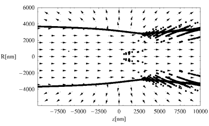
Figure 2: Structure of the quantum currents in the model of Eqs.(13,14,16) and parameters as specified in the text.

Ray-like structures in the right part of Fig.(2) correspond to the form taken by the separator locally near every Bragg angle. Important details of the separator structure are not discernible at this resolution, appearing only when we zoom very close to one Bragg angle. From Eq.(18) we can see that roots exist only if $G(\theta)$ satisfies $G(\theta)<C(D)$, where $C(D)$ is the maximum value of $R\mbox{e}^{-{R^{2}/2D^{2}}}$, equal to $D/\sqrt{\mbox{e}}$. Then the two roots $R_{1}(\theta)<D$ and $R_{2}(\theta)>D$ define a lower and un upper branch of the separator. Only the upper branch $R_{2}(\theta)$ is shown in Figure 2, since for most angles $\theta$ the lower branch corresponds to values of $R_{1}(\theta)$ smaller than $R_{2}(\theta)$ by many orders of magnitude.

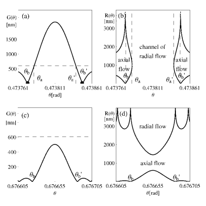
Figure 3: (a) The function $G(\theta)$ in a small neighborhood of the fourth Bragg angle $\theta_{q}=\theta_{4}=0.473811$rad. The horizontal dashed line corresponds to the level value $C(D)=De^{-0.5}=606.53$nm. The inner and outer separator curves are joined at the angles $\theta_{a}=0.4737825$rad and $\theta_{a}^{\prime}=0.4738395$rad, and a channel of radial flow is formed, of width $\Delta\theta=\theta_{a}^{\prime}-\theta_{a}=5.7\times 10^{-5}$rad. The function $G(\theta)$ becomes zero at the two closest zeros of the effective Fraunhofer function near the Bragg peak at $\theta_{q}=\theta_{4}$, namely at the angles $\theta_{b}=0.473773$ and $\theta_{b}^{\prime}=0.47385$. At these angles $R_{1}$ becomes zero while $R_{2}$ tends to infinity. (b) The form of the separator curves $R(\theta)$ in the same range of angles $\theta$ as in (a). (c,d) Same as in (a,b) but for a neighborhood of the Bragg angle $\theta_{q}=\theta_{8}=0.676655$.

The above picture changes very close to one Bragg angle $\theta_{q}$, where $R_{1}(\theta)$ becomes also important. This is because the local peaks of $|S_{eff}(\theta)|$ imply also local peaks of the function $G(\theta)$ in Eq.(18). According to the local value of the function $G(\theta=\theta_{q})$ we distinguish the following two cases:

Case I: $G(\theta_{q})>C(D)$. In this case there is an interval of values $\theta_{a}<\theta<\theta_{a}^{\prime}$ containing the Bragg angle $\theta_{q}$ such that Eq.(18) has no roots within it (Figure 3a). Then, the inner separator $R_{1}(\theta)$ of Fig.3b joins the outer separator $R_{2}(\theta)$ at the angles $\theta_{a}$ and $\theta_{a}^{\prime}$ and takes the form shown in Fig.3b (in coordinates $R$ vs. $\theta$). The gap between the left and right domains of prevalence of the ingoing flow corresponds to a narrow angular strip (hereafter called a ‘channel’) along which the flow is radial.

Case II: $G(\theta_{q})<C(D)$. In this case there are roots of both $R_{1}(\theta)$ and $R_{2}(\theta)$ for all angles $\theta$ surrounding and including $\theta_{q}$ (Fig.3c). However, $R_{1}(\theta)$ has a local maximum and $R_{2}(\theta)$ a local minimum at $\theta_{q}$ as well as on all other peaks caused by the side lobes of the Fraunhofer function. The separator then develops oscillations as shown in Fig.3d. Furthermore, in this case there may be one or more pairs of angles $(\theta,\theta^{\prime})$ where the inner, and outer, separator reaches the z-axis, and infinity, respectively. Two such pairs are visible in Fig.3d.

3.2 Nodal point - X-point complexes

Along the separator, a large number of quantum vortices are formed. Their location is given by all points where the conditions i) $\psi=0$, and ii)$\nabla\psi\neq 0$ hold. Such points are called nodal points. The condition $\psi=0$, or $\psi_{ingoing}=-\psi_{outgoing}$ yields, besides Eq.(18), a condition for the equality of phases, which takes the form (ignoring again $O(\hbar t/m)$ terms)

$$k_{0}R\tan(\theta/2)=2\bar{q}\pi~{}~{}~{}~{}~{}~{}~{}~{}\bar{q}\in{\cal Z}~{}~{}.$$ (19)

The pair of equations (18,19) specifies completely the coordinates of one nodal point(R,$\theta$). We locate many nodal points numerically by choosing different values of $\bar{q}$. It follows from Eq.(19) that the separation between two nearby nodal points, defined by two values $\bar{q}$ and $\bar{q}+1$, is of order $\pi/k_{0}\sim\lambda_{0}$.

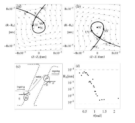
Figure 4: (a) Instantaneous form of the quantum flow around a nodal point placed at the left separator of the channel formed around the Bragg angle $\theta_{4}$ ($z_{0}=4505.7354$nm, $R_{0}=2310.6028$nm). The flow forms a ‘nodal point - X-point’ complex (Nodal point (N), X-point (X)) and follows in general one branch of the stable manifold (S) and then one branch of the unstable manifold (U) of the X-point. The other branches (SS,UU) are joined to form a loop. (b) Same as in (a) but for a nodal point placed on the right separator of the channel of $\theta_{4}$ ($z_{0}=4507.1939$, $R_{0}=2310.9549$nm). (c) Schematic representation of the quantum flow at the crossing of the channel, along with the directions of the stable and unstable manifolds of the X-points formed near the separator nodal points. The dashed lines represent the separator. (d) The size of some nodal point - X-point complexes, quantified by the distance $R_{X}$ from the nodal point to the X-point, as a function of $\theta$. The upper and lower dashed lines correspond to the estimates of Eq.(25) for the domains of Bragg angles and of diffuse scattering respectively.

The local form of the quantum flow in a very small neighborhood around one nodal point is very different from the general picture of the flow as given in Fig.2. If we ‘freeze’ the time $t$, the instantaneous pattern formed by the vector field of quantum probability current $\mathbf{j}$ corresponds to a characteristic structure called nodal point - X-point complex Efthymiopoulos et al. [2007]; Contopoulos & Efthymiopoulos [2008]; Efthymiopoulos et al. [2009]. That is, close to a nodal point we find a second critical point of the flow, where one has $\mathbf{j}=0$. This is called an ‘X-point’, since it can be shown that it is always simply unstable, i.e. there are two real eigenvalues of the matrix of the linearized flow around X, which are one positive and one negative. Accordingly, there are two opposite branches of unstable (U) and stable (S) manifolds emanating from X. On the other hand, the nodal point can be an attractor, center, or repellor. This determines the local form of the invariant manifolds U and S. It has been established theoretically Efthymiopoulos et al. [2007] that, except for a set of very small measure, most quantum trajectories avoid the nodal point, being instead scattered along the asymptotic directions of the manifolds of the X-point, leading to large distances from the nodal point - X-point complex. Furthermore, while, in general, the motion of nodal point - X-point complexes introduces chaos (Frisk [1997]; Wisniacki & Pujals [2005]; Efthymiopoulos et al. [2007, 2009]), in the present problem this effect is negligible because i) the speed of vortices is extremely small (of order $\sim\hbar/(k_{0}mD^{2})<<v_{0}$), and ii) the quantum trajectories exhibit only a finite number of encounters with nodal point - X-point complexes, as will be shown with numerical examples below. In conclusion, the effect of the nodal point - X-point complexes on the trajectories can be described as a scattering process without recurrences.

Figures 4a,b show two examples of such nodal point - X-point complexes, in which the central nodal points are located on the left side (Fig.4a) and right side (Fig.4b) respectively of the main channel around the fourth Bragg angle shown in Fig.3b. The stable and unstable manifolds of the X-points (found numerically) are shown like thick curves in the same figures. In Fig.4a, the left branch of the stable manifold is almost horizontal far from the X-point, while the right branch of the unstable manifold follows a radial direction which coincides with the direction defined by the local value of the scattering angle $\theta$. The other two branches form loops around the nodal point. If the terms $\hbar t/m$ in the wavefunction are ignored, the two branches join each other smoothly and the nodal point is a center. If however, all terms are taken into account, the nodal point is either an attractor or a repellor (see Efthymiopoulos et al. [2009]). Then one of the two branches in-spirals towards the nodal point, while the other deviates outwards after forming a nearly complete loop around the nodal point. In the present case, the time dependence of the wavefunction introduces negligible effects and the loops formed around all nodal points can be considered as practically closed. Then, in Fig.4a we see that, due to the form of the stable and unstable manifolds, trajectories approaching the X-point from the left in a nearly horizontal direction are scattered by the X-point. A scattered trajectory may or may not form a loop around the nodal point. In either case, the trajectories eventually recede from the X-point along the unstable manifold, and follow asymptotically a radial direction (upwards and to the right in Fig.4a). However, these directions are swapped in Fig.4b. The swapping can be understood with the help of a schematic figure (Fig.4c).

Details on the size of a nodal point - X-point complex are found by expanding the wavefunction $\psi$ as well as the Bohmian equations of motion in variables $u=z-z_{0}$, $v=R-R_{0}$ around a nodal point $(z_{0},R_{0})$.

Namely, from Eqs.(13,14), the wavefunction takes the form

$$\psi = \left[{1\over\sqrt{2}\pi}{D\over{\left(D^{2}+i\hbar t/m\right)^{1/2}}}e^{-ik_{0}^{2}\hbar t/2m}\right]\times\psi^{\prime}$$ (20)

where

$$\psi^{\prime}=e^{-{R^{2}\over 2(D^{2}+i\hbar t/m)}+ik_{0}z}-{\bar{P}S_{eff}(\theta)\over\sin^{2}(\theta/2)}{e^{ik_{0}r}\over r}$$ (21)

and $\bar{P}=(Z_{1}Ze^{2}m)/(8\pi\epsilon_{0}\hbar^{2})$. The prefactor in front of $\psi^{\prime}$ in Eq.(20) is simplified in the Bohmian equations of motion, which take the form

$${dz\over dt}={\psi^{\prime}_{*}(\partial\psi^{\prime}/\partial z)-\psi^{\prime}(\partial\psi^{\prime}_{*}/\partial z)\over\psi^{\prime}\psi^{\prime}_{*}},~{}~{}~{}~{}{dR\over dt}={\psi^{\prime}_{*}(\partial\psi^{\prime}/\partial R)-\psi^{\prime}(\partial\psi^{\prime}_{*}/\partial R)\over\psi^{\prime}\psi^{\prime}_{*}}~{}~{}.$$ (22)

Following Efthymiopoulos et al. [2009], the main characteristics of the equations of motion are found by the second order development of $\psi^{\prime}$ around a nodal point $(z_{0},R_{0})$. For $\bar{P}S_{eff}>0$ (as in the numerical parameters above), the condition $\psi^{\prime}(z_{0},R_{0})=0$ yields, if we disregard the term $i\hbar t/m$,

$$\bar{P}S_{eff}(\theta_{0})={R_{0}^{2}e^{-R_{0}^{2}/2D^{2}}\over 2(r_{0}+z_{0})},~{}~{}~{}e^{ik_{0}z_{0}}=e^{ik_{0}r_{0}}$$

where $r_{0}=\sqrt{R_{0}^{2}+z_{0}^{2}}$ and $\theta_{0}=\tan^{-1}(R_{0}/z_{0})$. Inserting this expression into the second order development of $\psi^{\prime}$,

$$\psi^{\prime}(u,v;z_{0},R_{0}) = (a_{10}+ib_{10})u+(a_{01}+ib_{01})v$$ (23)

$$+ {1\over 2}(a_{20}+ib_{20})u^{2}+{1\over 2}(a_{02}+ib_{02})v^{2}+(a_{11}+ib_{11})uv+\ldots,$$

where $u=z-z_{0}$, $v=R-R_{0}$, we find expressions for the coefficients $a_{10}$, $b_{10}$ ,$a_{01}$ ,$b_{01}$, $a_{20}$ ,$b_{20}$, $a_{02}$, $b_{02}$, $a_{11}$, $b_{11}$ (see Appendix B). The position of the X-point in the ‘adiabatic approximation’ (i.e. ignoring time variations of $\psi^{\prime}$) can be estimated (see equations (4) and (11) of Efthymiopoulos et al. [2009]) as:

$$0\simeq Av_{X}+B_{1}u_{X}^{2}+C_{1}v_{X}^{2}+D_{1}u_{X}v_{X}$$

$$0\simeq-Au_{X}+B_{2}u_{X}^{2}+C_{2}v_{X}^{2}+D_{2}u_{X}v_{X}$$ (24)

where

$$A=a_{01}b_{10}-a_{10}b_{01},$$

$$B_{1}={a_{02}b_{10}-a_{10}b_{02}\over 2},~{}~{}C_{1}={a_{02}b_{10}-a_{10}b_{02}-2a_{11}b_{01}\over 2},~{}~{}D_{1}=a_{02}b_{01}-a_{01}b_{02}$$

$$B_{2}={a_{01}b_{02}-a_{02}b_{01}\over 2},~{}~{}C_{2}={a_{01}b_{02}-a_{02}b_{01}-2a_{11}b_{10}\over 2},~{}~{}D_{2}=a_{10}b_{02}-a_{02}b_{10}~{}~{}.$$

The variational matrix at $(u_{X},v_{X})$ yielding the eigenvalues and eigenvectors at the X-point is determined by the same coefficients.

In Appendix B we estimate the size of all coefficients $a_{ij},b_{ij}$ near and far from Bragg angles. Using the set of equations (3.2) we then find an estimate for the quantity $R_{X}=(u_{X}^{2}+v_{X}^{2})^{1/2}$, i.e. for the size of a nodal point - X-point complex. The final result is

$$R_{X}=O\left({d\over Dk_{0}}\right)~{}~{} \mbox{domain of Bragg angles},~{}~{}~{}~{}$$ (25)

$$R_{X}=O\left({1\over Dk_{0}^{2}}\right)~{}~{} \mbox{domain of diffuse scattering}~{}.$$

Figure 4d shows the dependence of $R_{X}$ on $\theta$, obtained by computing numerically a sample of nodal point -X-point complexes along the separator at various angles $\theta$. The upper and lower dashed lines correspond to the upper and lower estimates of Eq.(25) respectively. We note that the transition from the validity of one estimate to the other occurs around the angle $\theta\approx 0.8$rad, This is nearly the angle beyond which the second term in the r.h.s. of Eq.(16) (diffuse scattering) becomes more important than the first term (coherent scattering).

4 Quantum trajectories. Emergence of the diffraction pattern

4.1 Trajectories

The results of the previous section will now be used in order to understand the form of Bohm’s trajectories of diffracted particles. A numerical calculation of a swarm of such trajectories is shown in Figure 5a. The initial conditions were chosen as $z_{0}=-10\mu$m, and $x_{0}$ taken uniformly in the interval $[1.5,3.3]\mu$m, for 360 trajectories. In Fig.5a a selective sample of trajectories is plotted so as to follow, at $t=0$ the distribution $dN/dR\propto R\mbox{e}^{-R^{2}/D^{2}}$, with $D=1\mu$m, corresponding to the choice of $\psi_{ingoing}$ as in Eq.(13). The numerical integration was done with adjustable time step of maximum value $\Delta t=0.1\pi\hbar/E$ (where $E=30$KeV) so as to ensure that the segment of a trajectory covered within one time step is significantly smaller than the wavelength $\lambda_{0}$.

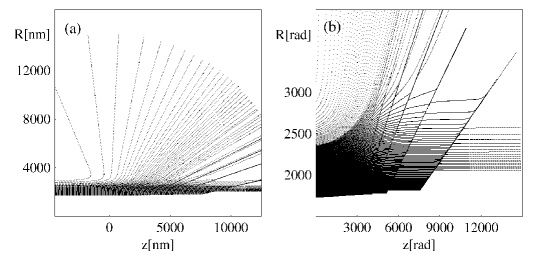
Figure 5: (a) A swarm of quantum trajectories (initial conditions: $z_{0}=-10^{4}$nm, $R_{0}$ in the interval $1.5\times 10^{3}$nm$\leq R_{0}\leq 3.3\times 10^{3}$nm). The plot shows a sample of trajectories selected by their values of $R_{0}$ being distributed according to ${\Delta N\over\Delta R}\propto 2\pi R\mbox{e}^{-R^{2}/D^{2}}$ which corresponds to the choice of $\psi_{ingoing}$ as in Eq.(13). (b) A zoom of (a) in the region where the trajectories are forced to follow a diffraction pattern by crossing the channels of consecutive Bragg angles. The sharp deflections seen correspond to the Bragg angles $\theta_{q}$, $q=1,...,8$ (right to left).

The main feature of Fig.5a is that the trajectories with larger initial normal distance $R_{0}$ from the z-axis are deflected to larger angles $\theta$. This effect is in contrast to the picture of classical Rutherford scattering and it can be regarded as a clear manifestation of the quantum character of diffraction for a large transverse quantum coherence length. Such behavior of the quantum trajectories is readily accounted for by the fact that the average inclination of the separator in the $(z,R)$ plane is negative. Namely, since all trajectories are horizontal until they encounter the separator, trajectories of larger initial $R_{0}$ encounter the separator at a larger angle $\theta$ satisfying Eq.(18) with $R=R_{0}$(Fig.1a). We thus have that $\theta$ is an increasing function of $R_{0}$.

Figure 5b shows now a zoom in the domain of forward-scattered trajectories, leading to the formation of a diffraction pattern. The trajectories that started closer to the z-axis follow initially the general flow due to $\psi_{ingoing}$, but they are subject to abrupt deflections at the crossing of any Bragg angle. Such deflections are due to the entering of the trajectories into channels of radial flow. This effect is depicted in detail in Figure 6a, showing only one trajectory that suffers five consecutive deflections by passing through consecutive channels of radial flow before exiting to the domain of prevalence of the radial flow leading to the first Bragg angle $\theta_{q}=\theta_{1}=0.23$. A comparison of the deflections at the Bragg angles $\theta_{q}=\theta_{2}$ and $\theta_{q}=\theta_{1}$ is shown in panels (b) and (c) of the same figure, where the coordinates are locally rotated so that the vertical axis always coincides with the radial direction. We clearly see the channels of radial quantum flow formed around each Bragg angle. The dashed vertical lines show local segments of the separator lines which mark essentially the limits of the channels in either case. The deflection of an orbit is caused at the crossing of the separator, and it is due to the orbit necessarily following the flow around the X-points that exist along the separator. The deflection causes a trajectory to follow a path nearly parallel to the radial direction, albeit with a small transverse angle, as in Fig.6b, due to $\psi_{ingoing}$, which still has some (small) influence in that region of the channel. Then there are two possibilities: i) the trajectory traverses the whole channel and exits from it from the side opposite to the entry, regaining almost horizontal flow afterwards (Fig.6b), or ii) the orbit is entrained by the channel all along its length, in which case the particle exits from the scattering domain to infinity along the Bragg angle associated with that particular channel (Fig.6c).

Figure 6: (a) One quantum trajectory (bold), initial conditions $(z_{0},R_{0})=(-10000$nm$,1865$nm$)$, which exits from the first Bragg angle after a number of visible consecutive encounters with the channels of subsequent Bragg angles (solid lines). (b) The crossing of the channel of the second Bragg angle $\theta_{q}=\theta_{2}=0.33345266$ as viewed in locally rotated coordinates $x_{1}=z\cos(\pi/2-\theta_{2})-R\sin(\pi/2-\theta_{2})$, $x_{2}=z\sin(\pi/2-\theta_{2})+R\cos(\pi/2-\theta_{2})$. Note the different scale on the axes. The arrows indicate the local direction of the quantum flow, which changes abruptly in a narrow zone near $x_{1}=0$, corresponding to $\theta$ being exactly equal to the Bragg value. The dashed vertical lines indicate the positions of the pair of closest zeros to the peak of the effective Fraunhofer function near $\theta=\theta_{2}$. (c) Same as in (b) but for the crossing of the channel of the first Bragg angle $\theta_{q}=\theta_{1}=0.23523778$. In this case the trajectory never reaches the right border of the channel.

Since $\psi_{ingoing}$ is larger closer to the z-axis, the orbits that started closer to the z-axis have larger probability to cross more channels and end either with horizontal motion, or radial motion along the direction of one of the first Bragg angles. This leads to a complete stratification of the flow as shown in Fig.5. On the other hand, due to attenuation effects (section 2) the channels practically disappear beyond some Bragg angle and the separator takes locally the form of Fig.3d, with oscillations of smaller and smaller amplitude. This causes a gradually smaller concentration of the exiting trajectories around the Bragg angles $\theta_{q}$ with high $q$ , leading eventually to a diffuse form of the radial outward flow at large angles $\theta$.

5 Times of flight

An important practical utility of the quantum trajectory approach regards the possibility to unambiguously determine the times of flight of particles, i.e. the time it takes for a particle to travel between an emitter surface and a detector surface. This question is of particular interest, because it is related to a well known open problem of quantum theory, namely the so-called ‘problem of time’ (see Muga & Leavens [2000]; Muga et al. [2002] for reviews). This problem stems from a theorem of Pauli Pauli [1926], according to which it is not possible to properly define a self-adjoint time operator consistent with all axioms of quantum mechanics. This implies that the usual (Copenhagen)) formalism based on state vectors or density matrices is not applicable to a quantum-theoretical calculation of probabilities related to time observables (e.g. the distribution of arrival times to a detector or the times of flight defined as above). In fact, in standard quantum mechanics (i.e. in both Schrödinger’s and Heisenberg’s pictures), time is considered only as a parameter of the quantum equations of motion.

Among various proposals in the literature aiming to remedy this gap of standard quantum theory (Muga & Leavens [2000]), the Bohmian formalism offers a straightforward solution, since the time of flight is well-defined along the Bohmian trajectories. This is in principle subject to experimental testing, and one such test will be proposed below. We note in passing two other approaches on the same subject, namely the ‘history approach’, based on Feynman paths, and the Kijowski approach (Kijowski [1974]), based on so-called ‘Bohm-Aharonov (Hartle [1988]; Yamada & Takagi [1993]) operators. However these approaches have not been so far as clearly formulated as the Bohmian formulation.

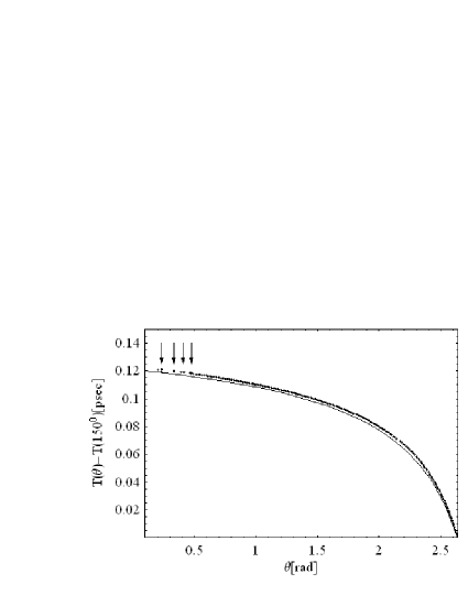
Figure 7: The difference $T(\theta)-T(150^{\circ})$ of the arrival times of particles to detectors placed at the angles $\theta$ and $150^{\circ}$ respectively and at the same distance from the center, for the quantum trajectories of Fig.5a. The solid curve corresponds to the analytic estimate of Eq.(26). The arrows correspond to the first four Bragg angles.

A calculation of the times of flight in the case of the trajectories of Fig.5 can be done as follows. We note first that, as a simple visual inspection of of Fig.5 shows, starting from a fixed horizontal distance from the left (source), the trajectories that are deflected to large angles are shorter in length than the trajectories deflected to small angles, provided that the final detection point is at the same distance $r$ from the center. We can quantify this difference by approximating the form of the trajectories as horizontal up to their deflection at the outer separator and radial afterwards. The modulus of the velocity remains nearly constant $v\simeq\hbar k_{0}/m$ in both the horizontal and radial segments of the trajectory. Taking into account the separator equation (Eq.(18)), we estimate the length, and hence the time difference between two trajectories deflected at two arbitrary angles $\theta_{1}$ and $\theta_{2}$ by a simple geometric analysis. If the separator is approximated by a straight line between the two angles (e.g. in the forward and backward directions $\theta_{1}=30^{\circ}$, $\theta_{2}=150^{\circ}$) we find:

$$T(\theta_{1})-T(\theta_{2})\approx{m\over\hbar k_{0}}\left({(R_{0,2}+\lambda(\theta_{1}-\theta_{2})(\cos\theta_{1}-1)\over\sin\theta_{1}}-{R_{0,2}(\cos\theta_{2}-1)\over\sin\theta_{2}}\right)$$ (26)

where the slope $\lambda$ is normalized to its value for the pair $(\theta_{1},\theta_{2})=(30^{\circ},150^{\circ})$ namely

$$\lambda={R_{0,2}-R_{0,1}\over\theta_{2}-\theta_{1}}$$

with $R_{0,j}$, $j=1,2$ calculated by Eq.(18) with $\theta$ substituted by $\theta_{1}$ and $\theta_{2}$ respectively.

Eq.(26) agrees well with a numerical computation of the times of flight for various angles $\theta$ (see Fig.7). The main remark is that, since $R_{0}\propto D$ (cf. Eq.(18)), the time difference $T(\theta_{1})-T(\theta_{2})$ for two fixed angles is proportional to the transverse quantum coherence length $D$. That is, Eq.(26) leads to the estimate $T(\theta_{1})-T(\theta_{2})=O(D/v_{0})$. This is a relation that can be tested experimentally. In fact, it is very different to what is found in the case of Rutherford scattering (compare Figs.1a and 1b), where a straightforward analysis yields

$$T(\theta_{1})-T(\theta_{2})\approx{ZZ_{1}e^{2}\over 2\pi\epsilon_{0}mv_{0}^{3}}\ln\left(\sqrt{1+\cot^{2}(\theta_{2}/2)\over 1+\cot^{2}(\theta_{1}/2)}\right)$$ (27)

i.e. the time difference $T(\theta_{1})-T(\theta_{2})$ does not depend on the transverse quantum coherence length $D$ and it has a different dependence $O(1/v_{0}^{3})$, rather than $O(D/v_{0})$, on the particles’ velocities. In the case of electrons, the classical time difference is of order $10^{-20}sec$, while, assuming $D\sim 10^{-6}m$ the quantum time difference is of order $10^{-12}sec$. We note that the latter time-resolution scale is within present-day experimental possibilities. However, in order that the experiment becomes feasible, one should be able to combine very accurate time measurements with single-electron detectors (see Steinberg [2008] for a review of recent experimental techniques on quantum-mechanical time measurements). Furthermore, one should also be able to have a control signal for the emission times of electrons. This is a largely unexplored subject (one possibility is probably offered by the so-called LASER induced field emission; see Barwick et al. [2007]). At any rate, in view of theoretical results like the above, we think it is safe to anticipate that the advent of experimental time measurement techniques in systems with a genuinely quantum behavior will open a new window for probing quantum mechanics at a very fundamental level.

6 Conclusions

We applied the method of the de Broglie - Bohm quantum trajectories in the problem of charged particle diffraction from thin material targets, focusing on the case of significant transverse quantum coherence of the particle beam, where new genuinely quantum phenomena appear. In particular:

1) We constructed a model for the wavefunction of diffracted particles which takes into account both processes of coherent (giving rise to Bragg angles) and diffuse scattering.

2) We developed a theory for the quantum-current structure near a locus called separator, i.e. the border between an inner tube of ingoing flow surrounding the beam’s axis of symmetry and an outer domain, where the radial outward flow prevails. Analytical expressions are found for the separator. The separator forms thin channels of radial flow very close to every Bragg angle. Such channels are responsible for the concentration of quantum trajectories to particular directions of exit from the ingoing flux tube.

3) The deflection of quantum trajectories is due to their interaction with an array of quantum vortices formed around a large number of nodal points located on the separator. The quantum flow near every nodal point takes the form of a ‘nodal point - X-point complex’. The size of quantum vortices is estimated analytically close to and far from Bragg angles, the estimate being in close agreement with numerical results.

4) The emergence of a diffraction pattern is explained in terms of numerically calculated quantum trajectories. In particular, we demonstrate the sharp deflections of the trajectories as they approach one or more X-points along the latters’ stable manifolds, and recede from these points along their unstable manifolds. The radically non-classical character of the quantum trajectories is demonstrated. We find that trajectories with larger initial distance $R_{0}$ from the central axis of the ingoing flux tube (i.e. larger impact parameter) are deflected to larger angles $\theta$. This is contrary to the classical Rutherford scattering, where the trajectories with larger impact parameter are deflected to smaller angles $\theta$.

5) The times of flight $T(\theta)$ of particles to detectors placed at constant distances and various angles $\theta$ from the target are calculated by an analytical approximation and compared to numerical results. It is demonstrated that the time difference $T(\theta_{1})-T(\theta_{2})$ follows the scaling $T(\theta_{1})-T(\theta_{2})=O(D/v_{0})$, where $D$ is the transverse quantum coherence length and $v_{0}$ the average particles’ velocity. This scaling is different than in classical Rutherford scattering where $T(\theta_{1})-T(\theta_{2})=O(|ZZ_{1}|e^{2}/(2\pi\epsilon_{0}mv_{0}^{3}))$ and it leads to the possibility of an experimental test of the Bohmian formalism in a sector of quantum theory where the Copenhagen approach offers no standard recipe, i.e. the sector of time observables. Acknowledgments C. Delis was supported by the State Scholarship Foundation of Greece (IKY) and by the Hellenic Center of Metals Research.

Effective Fraunhofer function

We consider the simplest example of a cubic lattice arrangement of the atoms in the target. The atomic positions $\mathbf{r}_{j}$ are given by:

$$\mathbf{r}_{j}=(n_{x},n_{y},n_{z})a+\Delta a\mathbf{u}_{j}(t),$$ (28)

$$(n_{x},n_{y},n_{z}) \in (-{N_{\perp}\over 2},{N_{\perp}\over 2})\times(-{N_{\perp}\over 2},{N_{\perp}\over 2})\times(-{N_{z}\over 2},{N_{z}\over 2})$$

where $a$ is the lattice constant (equal to the length of one side of the primitive cell), $\Delta a$ is the amplitude of random oscillations (due to thermal or recoil motions; $\Delta a$ is taken equal to a small fraction of $a$) and $\mathbf{u_{j}}\equiv(u_{j,x},u_{j,y},u_{j,z})$ are random variables with a uniform distribution in the intervals $[-0.5,0.5]$. The number of atoms $N_{z}$ in the z-direction is $N_{z}=d/a$, where $d$ is the target thickness. On the other hand, the value of $N_{\perp}$ can be chosen as $N_{\perp}=D/a$, since by such a choice the value of the Gaussian weight in Eq.(15) can be approximated by $\approx 1$ for all $|n_{x}|<N_{\perp}/2$ and $|n_{y}|<N_{\perp}/2$, and $\approx 0$ for $|n_{x}|>N_{\perp}/2$ or $|n_{y}|>N_{\perp}/2$. Given these approximations, we find a model for the effective Fraunhofer function (Eq.(15)) accounting for diffraction effects when $k_{0}a\sim 1$ (if $k_{0}a>>1$ the diffraction effects disappear). In this case we have

$$S_{eff}(k_{0};\mathbf{r})\approx\sum_{n_{z}=-N_{z}/2}^{N_{z}/2}\sum_{n_{x}=-N_{\perp}/2}^{N_{\perp}/2}\sum_{n_{y}=-N_{\perp}/2}^{N_{\perp}/2}e^{2ik_{0}(n_{z}a+\Delta au_{z})\sin^{2}(\theta/2)}$$

$$\times e^{-i[(n_{x}a+\Delta au_{x})\sin\theta\cos\varphi-(n_{y}a+\Delta au_{y})\sin\theta\sin\varphi]}$$ (29)

Equation (6) is still not convenient for a practical use in numerical calculations, since the triple sum in the r.h.s. has a prohibitive cost to compute. However, a drastic simplification takes place by considering a material target having a polycrystalline structure. In this case, we can effectively proceed by randomizing the value of $\varphi$ in the terms of (6) (which is mathematically equivalent to considering random rotations of small crystallites, on planes normal to the beam). In this case, the dependence of the sum in Eq.(6) on $u_{x}$, $u_{y}$ effectively disappears, since the corresponding terms in the exponential argument are effectively dominated by the random variations due to $\varphi$. Furthermore, since $u_{z}$ is also random, the distribution of values of $S_{eff}$ for different samples of values $(u_{x},u_{y},u_{z})$ becomes practically equivalent to the distribution of values of the quantity

$$S_{eff}(k_{0};\mathbf{r})\approx\sum_{n_{z}=-N_{z}/2}^{N_{z}/2}e^{2ik_{0}(n_{z}a+\Delta au_{z})\sin^{2}(\theta/2)}$$

$$\times\sum_{n_{x}=-N_{\perp}/2}^{N_{\perp}/2}\sum_{n_{y}=-N_{\perp}/2}^{N_{\perp}/2}e^{-i[(n_{x}a+\Delta au_{x})\sin\theta\cos\varphi-(n_{y}a+\Delta au_{y})\sin\theta\sin\varphi]}$$ (30)

i.e. where the triple sum is decomposed to a $1\times 2$ sum. Denoting by $S_{xy}$ an rms value of the double sum in (6), we find that $S_{xy}$ is of order $N_{\perp}\sim D/a$. We then substitute $S_{xy}=(D/a)C_{coherent}$, where $C_{coherent}$ is a fitting constant, in the place of the double sum. Equation (6) takes the form

$$S_{eff}(\theta)\approx(D/a)e^{i\delta}\sum_{n_{z}=-N_{z}/2}^{N_{z}/2}C_{coherent}\exp(i2k_{0}(n_{z}a+\Delta au_{n_{z}})\sin^{2}(\theta/2))$$ (31)

where $\delta$ is a random phase. The value of the fitting constant $C_{coherent}$ is determined numerically by running a realization of the sums appearing in (31) in the computer, and comparing the computed quantities with the results with the full sum (6) for various values of $N_{\perp}$ and $N_{z}$. To arrive at a final fitting model, we note first that if the noise is taken equal to zero ($u_{n_{z}}=0$), the form of $S_{eff}$ near an angle $\theta_{q}$ is:

$$S_{q,eff}(\theta)\approx(D/a)e^{i\delta}C_{coherent}\frac{2\sin\left[k_{0}N_{z}a\sin(\theta_{q})(\theta-\theta_{q})/2\right]}{k_{0}a\sin(\theta_{q})(\theta-\theta_{q})}~{}~{}.$$ (32)

Taking now into account the noise, the attenuation of the maxima can be estimated by a Debye-Waller factor (see e.g. Peng [2005]), changing (32) into

$$S_{q,eff}(\theta)\approx$$

$$(D/a)e^{i\delta}C_{coherent}\exp\left(-{1\over 2}4k_{0}^{2}\sin^{4}(\theta/2)\sigma_{a}^{2}\right)\frac{2\sin\left[k_{0}N_{z}a\sin(\theta_{q})(\theta-\theta_{q})/2\right]}{k_{0}a\sin(\theta_{q})(\theta-\theta_{q})}$$ (33)

Equation (6) yields the form of the Fraunhofer function locally, very close to a Bragg angle. The total ‘coherent’ contribution to the Fraunhofer function is a sum of terms like (6) over all Bragg angles:

$$S_{coherent}(\theta)\approx$$

$$(D/a)e^{i\delta}\sum_{q=0}^{q_{max}}C_{coherent}\exp\left(-{1\over 2}4k_{0}^{2}\sin^{4}(\theta/2)\sigma_{a}^{2}\right)\frac{2\sin\left[k_{0}N_{z}a\sin(\theta_{q})(\theta-\theta_{b})/2\right]}{k_{0}a\sin(\theta_{q})(\theta-\theta_{q})}~{}~{}$$ (34)

where $q_{max}$ is the total number of Bragg angles. To this we add a ‘diffuse’ term accounting for random phasor sums away from all Bragg angles. We have $S_{diffuse}\sim N_{\perp}N_{z}^{1/2}$, weighted by the complement of the Debye-Waller factor $1-e^{-{1\over 2}4k_{0}^{2}\sin^{4}(\theta/2)\sigma_{a}^{2}}$. Thus, a final model for the Fraunhofer function reads:

$$S_{eff}(\theta) = {De^{i\delta}\over a}\Bigg{[}\sum_{q=0}^{q_{max}}C_{coherent}e^{-{1\over 2}4k_{0}^{2}\sin^{4}(\theta/2)\sigma_{a}^{2}}\frac{2\sin\left[k_{0}N_{z}a\sin(\theta_{q})(\theta-\theta_{q})/2\right]}{k_{0}a\sin(\theta_{q})(\theta-\theta_{q})}$$ (35)

$$+ (1-e^{-{1\over 2}4k_{0}^{2}\sin^{4}(\theta/2)\sigma_{a}^{2}})C_{diffuse}\sqrt{N_{z}}\Bigg{]}$$

where $C_{diffuse}$ is also a fitting constant specified numerically. Substituting $N_{z}=d/a$ we obtain Eq.(16).

Size of quantum vortices

Starting from Eq.(23), we obtain an estimate of the size of the coefficients $a_{ij}$, $b_{ij}$ near and far from Bragg angles as follows: For an angle $\theta_{0}$ close to a Bragg angle, using the definition (32), one has for the derivatives of $S_{eff}(\theta)$ the following estimates:

$${dS_{eff}\over S_{eff}d\theta_{0}}\sim{N_{z}k_{0}a}\sim k_{0}d,~{}~{}~{}{d^{2}S_{eff}\over S_{eff}d\theta_{0}^{2}}\sim{N_{z}^{2}k_{0}^{2}a^{2}}\sim(k_{0}d)^{2}~{}~{}.$$

Since $d/D<<1$, from the above expressions we find the dominant terms of all the coefficients $a_{ij}$, $b_{ij}$. These are:

$$a_{10}=e^{-R_{0}^{2}/2D^{2}}\bigg{[}-\sin(k_{0}z_{0})k_{0}(1-\cos\theta_{0})+O(k_{0}d/D)\bigg{]}$$

$$b_{10}=e^{-R_{0}^{2}/2D^{2}}\bigg{[}\cos(k_{0}z_{0})k_{0}(1-\cos\theta_{0})+O(k_{0}d/D)\bigg{]}$$ (36)

$$a_{01}=e^{-R_{0}^{2}/2D^{2}}\bigg{[}\sin(k_{0}z_{0})k_{0}\sin\theta_{0}+O(k_{0}d/D)\bigg{]}$$

$$b_{01}=e^{-R_{0}^{2}/2D^{2}}\bigg{[}-\cos(k_{0}z_{0})k_{0}\sin\theta_{0}+O(k_{0}d/D)\bigg{]}$$

$$a_{20}=e^{-R_{0}^{2}/2D^{2}}\bigg{[}-\cos(k_{0}z_{0}){k_{0}^{2}\over 2}\sin^{2}\theta_{0}+O(k_{0}^{2}d^{2}/D^{2})\bigg{]}$$

$$b_{20}=e^{-R_{0}^{2}/2D^{2}}\bigg{[}-\sin(k_{0}z_{0}){k_{0}^{2}\over 2}\sin^{2}\theta_{0}+O(k_{0}^{2}d^{2}/D^{2})\bigg{]}$$

$$a_{02}=e^{-R_{0}^{2}/2D^{2}}\bigg{[}\cos(k_{0}z_{0}){k_{0}^{2}\over 2}\sin^{2}\theta_{0}+O(k_{0}^{2}d^{2}/D^{2})\bigg{]}$$ (37)

$$b_{02}=e^{-R_{0}^{2}/2D^{2}}\bigg{[}\sin(k_{0}z_{0}){k_{0}^{2}\over 2}\sin^{2}\theta_{0}+O(k_{0}^{2}d^{2}/D^{2})\bigg{]}$$

$$a_{11}=e^{-R_{0}^{2}/2D^{2}}\bigg{[}\cos(k_{0}z_{0}){k_{0}^{2}\over 2}\sin 2\theta_{0}+O(k_{0}^{2}d^{2}/D^{2})\bigg{]}$$

$$b_{11}=e^{-R_{0}^{2}/2D^{2}}\bigg{[}\sin(k_{0}z_{0}){k_{0}^{2}\over 2}\sin 2\theta_{0}+O(k_{0}^{2}d^{2}/D^{2})\bigg{]}$$

The quantities $r_{0},z_{0},R_{0}$ are all of order $O(D)$. The equalities $a_{20}=-a_{02}$, and $b_{20}=-b_{02}$ (to leading order) are due to the fulfilment of the continuity equation by the wavefunction $\psi$ (see Efthymiopoulos et al. [2009]). However, since the outgoing term was evaluated only up to $O(\sigma_{\perp}^{2}/k_{0}^{2})=O(1/D^{2}k_{0}^{2})$, the above equalities are also violated at the same order, resulting in a small relative error (of order $10^{-6}$). Substituting these expressions into Eq.(3.2), we remark that the products of the leading terms of the coefficients $a_{10},b_{10},a_{01},b_{01}$ cancel exactly in the coefficient $A$ (while they do not cancel in all other contributions). As a result, near a Bragg angle one has

$$A=O\left({k_{0}^{2}d\over D}\right),~{}~{}B_{i}=O(k_{0}^{3}),~{}~{}C_{i}=O(k_{0}^{3}),~{}~{}D_{i}=O(k_{0}^{3}),~{}~{}i=1,2$$

whence, in view of (3.2),

$$u_{X}=O\left({d\over Dk_{0}}\right),~{}~{}~{}~{}v_{X}=O\left({d\over Dk_{0}}\right)~{}~{}.$$ (38)

Substituting the above estimates in the expression $R_{X}=(u_{X}^{2}+v_{X}^{2})^{1/2}$ we find the first of Eqs.(25).

On the other hand, far from Bragg angles all the terms with derivatives $dS_{eff}/d\theta_{0}$, $d^{2}S_{eff}/d\theta_{0}^{2}$ in the equations specifying the coefficients $a_{ij},b_{ij}$ become negligible. Then, we have precisely the same leading terms in all the coefficients $a_{ij},b_{ij}$ as before. In the subsequent order, however, the terms are $O(1/D)$ for the coefficients $a_{10},b_{10}$, $a_{01},b_{01}$, and $O(k_{0}/D)$ for the coefficients $a_{20},b_{20}$, $a_{11},b_{11}$, $a_{02},b_{02}$. Then

$$A=O\left({k_{0}\over D}\right),~{}~{}B_{i}=O(k_{0}^{3}),~{}~{}C_{i}=O(k_{0}^{3}),~{}~{}D_{i}=O(k_{0}^{3}),~{}~{}i=1,2$$

Thus

$$u_{X}=O\left({1\over Dk_{0}^{2}}\right),~{}~{}~{}~{}v_{X}=O\left({1\over Dk_{0}^{2}}\right)~{}~{}$$ (39)

which, upon substitution to $R_{X}=(u_{X}^{2}+v_{X}^{2})^{1/2}$ leads to the second of the estimates (25).

References

- Barwick et al. [2007] Barwick, B., Corder, C., Strohaber, J., Chandler-Smith, N., Uiterwaal, C., & Batelaan, H. 2007, New Journal of Physics, 9, 142
- Beenakker & van Houten [1991] Beenakker, C.W., and van Houten, H.: 1991, Solid State Phys. 44, 1.
- Bennett [2010] Bennett, A.: 2010, J. Phys. A 43, 5304.
- Bohm [1952] Bohm, D.: 1952,Phys. Rev. 85, 166; 85 194.
- Colin & Struyve [2010] Colin, S., and Struyve, W.: 2010, New J. Phys. 12, 3008.
- Contopoulos & Efthymiopoulos [2008] Contopoulos, G., and Efthymiopoulos, C.:2008, Celest. Mech. Dyn. Astron. 102, 219.
- De Broglie [1925] De Broglie, L.: 1925,Ann. Phys. Paris 3, 22.
- Delis et al. [2011] Delis, N., Efthymiopoulos C., and Contopoulos, G.: 2011, ‘Wavepacket approach to electron diffraction: Bohmian trajectories and arrival times’ (in preparation).
- Efthymiopoulos & and Contopoulos [2006] Efthymiopoulos C., and Contopoulos, G.: 2006, J. Phys. A 39, 1819.
- Efthymiopoulos et al. [2007] Efthymiopoulos, C., Kalapotharakos, C., and Contopoulos, G.: 2007, J. Phys. A 40, 12945.
- Efthymiopoulos et al. [2009] Efthymiopoulos, C., Kalapotharakos, C., and Contopoulos, G.: 2009, Phys. Rev. E 79, 036203.
- Frisk [1997] Frisk, H.: 1997, Phys. Lett. A 227, 139.
- Gindensperger [2003] Gindensperger, E.: 2003, Phys. Rev. D37, 2818.
- Hartle [1988] Hartle, J.B.: 1988, Phys. Rev. D37, 2818.
- Kijowski [1974] Kijowski, J: 1974, Rev. Mod. Phys. 6, 361.
- Lopreore [1999] Lopreore, C.L. and Wyatt, R.E.: 1999, Phys. Rev. Lett. 82, 5190.
- Madelung [1926] Madelung, E: 1926,Z. Phys. 40, 332.
- Muga & Leavens [2000] Muga, J.G., and Leavens, C.R.: 2000, Phys. Rep. 338, 353.
- Muga et al. [2002] Muga, J.G., Sala Mayato, R., and Egusquiza I.L.: 2002, Lect. Notes Phys. 72, 1.
- Oriols [2007] Oriols, X: 2007, Phys. Rev. Lett. 98, 066803.
- Pauli [1926] Pauli, W: 1926, Hanbuch der Physik 22, pp.1-278, Springer, Berlin.
- Peng et al. [2004] Peng, L.M., Dudarev, S.L., and Whelan, M.J.: 2004, High-Energy Electron Diffraction and Microscopy, Oxford University Press, Oxford.
- Peng [2005] Peng, L.M.: 2005, J. El. Micr. 54, 199.
- Philippidis et al. [1979] Philippidis, C., Dewdney, C. and Hiley, B.: 1979, Nuovo Cimento B 52, 15.
- Sanz et al. [2002] Sanz, A.S., Borondo, F., and Miret-Artés, S: 2002, J. Phys.: Condens. Matter 14, 6109.
- Sanz et al. [2004] Sanz,A.S., Borondo, F., and Miret-Artés, S: 2004, J. Chem. Phys. 120, 8794.
- Steinberg [2008] Steinberg, A.S.: 2008, Lect. Notes Phys. 734, 333.
- Vallentini & and Westman [2005] Vallentini, A., and Westman, H.: 2005, Royal Soc. London Proc. A 461, 253.
- Wyatt [2005] Wyatt, R.: 2005,Quantum Dynamics with Trajectories, Springer, New York.
- Wisniacki & Pujals [2005] Wisniacki, D.A., and Pujals, E.R.: 2005, Europhys. Lett. 71, 159.
- Yamada & Takagi [1993] Yamada, N. and Takagi, S.: 1993, Prog. Theor. Phys. 86, 599.
- Zhao & Makri [2003] Zhao, Y., and Makri, N.: 2003, J. Chem. Phys. 119, 60.