Higher particle form factors of branch point twist fields in integrable quantum field theories
Olalla A. Castro-Alvaredo and Emanuele Levi
Centre for Mathematical Science, City University London,
Northampton Square, London EC1V 0HB, UK
In this paper we compute higher particle form factors of branch point twist fields. These fields were first described in the context of massive 1+1-dimensional integrable quantum field theories and their correlation functions are related to the bi-partite entanglement entropy. We find analytic expressions for some form factors and check those expressions for consistency, mainly by evaluating the conformal dimension of the corresponding twist field in the underlying conformal field theory. We find that solutions to the form factor equations are not unique so that various techniques need to be used to identify those corresponding to the branch point twist field we are interested in. The models for which we carry out our study are characterized by staircase patterns of various physical quantities as functions of the energy scale. As the latter is varied, the -function associated to these theories comes close to vanishing at several points between the deep infrared and deep ultraviolet regimes. In other words, renormalisation group flows approach the vicinity of various critical points before ultimately reaching the ultraviolet fixed point. This feature provides an optimal way of checking the consistency of higher particle form factor solutions, as the changes on the conformal dimension of the twist field at various energy scales can only be accounted for by considering higher particle form factor contributions to the expansion of certain correlation functions. o.castro-alvaredo@city.ac.uk emanuele.levi.1@city.ac.uk
1 Introduction
Entanglement is the most distinct and bizarre of all quantum phenomena. The idea that the quantum states of objects so wide apart from each other that they are not even causally connected can be entangled seems counterintuitive and has been hotly debated [1]. Although the interpretation of quantum mechanics and quantum entanglement continues to be discussed, the reality of entanglement as a physical phenomenon was finally established through the experiments of Alain Aspect and his collaborators [2]. In addition, in recent years, entanglement has started to reveal its powerful practical applications, specially in the context of quantum computation, quantum cryptology and quantum teleportation (see e.g. [3, 4]).
From a theoretical point of view entanglement is intimately linked to the structure of quantum states so that developing methods to “measure” entanglement is a very efficient way to learn more about the fundamental properties of quantum systems. In that sense, many different theoretical measures of entanglement have been proposed in the literature [5, 6, 7, 8, 9] of which the entanglement entropy [5] is just an example. In recent years much work has been carried out to compute the entanglement entropy of extended quantum systems with many degrees of freedom, such as quantum spin chains [10, 11, 12, 13, 14, 15, 16, 17, 18, 19, 20] and quantum field theories [21, 22, 23, 24, 25].
Consider a quantum system, with Hilbert space , in a pure state . The bi-partite entanglement entropy is the von Neumann entropy [26] associated to the reduced density matrix of the subsystem , , defined as
| (1.1) |
One way of interpreting is to understand it as a measurement of the entanglement of the quantum state of subsystem when the latter is considered in isolation (ignoring the existence of subsystem ).
In a series of recent works involving one of the present authors [24, 27, 28, 25] a new approach to the computation of (1.1) for 1+1-dimensional integrable quantum field theories (QFT) has been proposed and developed. This approach takes as starting point the “replica trick”. This consists of replacing the theory under scrutiny by a new model consisting of non-interacting copies or “replicas” of the original theory. Although this might seem to lead to an unnecessary complication of the problem, it does in fact simplify it by producing a new theory which possesses an extra symmetry under cyclic permutations of the -copies of the model. Associated to this symmetry there exists a special class of twist fields and which have been named branch point twist fields. The key result is
| (1.2) |
that is, the trace of the density matrix of the replica theory is proportional to the two-point function of twist fields. is the size of subsystem in the quantum field theory. Therefore, once the trace has been computed, the von Neumann entropy follows from the identity,
| (1.3) |
This identity does however involve a highly non-trivial analytic continuation of the function to positive non-integer values of which makes the limit above extremely hard to compute [24, 27, 28]. It is sometimes more convenient to compute another type of entanglement entropy known as Rényi entropy [29] which is given by
| (1.4) |
and whose limit gives (1.1) once more.
In the current work we wish to take the identity (1.2) as our main motivation to investigate the form factors of the twist field . As is well known, the correlation function in (1.2) can be expanded in terms of form factors of the fields involved. Therefore knowing the form factors allows us in principle to extract both the von Neumann and Rényi entropies of any integrable QFT under consideration.
This paper is organised as follows: In section 2 we summarise the form factor programme for branch point twist fields [24]. In section 3 we introduce the -sum rule [30] and the two models which we want to study in detail: the roaming trajectories (RT) model and the -homogenous sine-Gordon (HSG) model. In section 4 we describe in detail the construction of higher particle form factors for the RT-model. We place special emphasis on the existence of multiple solutions to the form factor equations. We successfully apply the cluster decomposition property to identify those that must correspond to the branch point twist field which is related to the bi-partite entanglement entropy of the model. In section 5 we carry out a similar analysis for the -HSG model concentrating less on the non-uniqueness of solutions and more on the extra challenges posed by the more complex particle spectrum of the model. In section 6 we provide numerical results for the ultraviolet conformal dimension of the twist field in the RT- and HSG-model which are fully consistent with the theoretical predictions. We present our conclusions in section 7.
2 Form factors of branch point twist fields
In this paper we will be concerned with the computation of matrix elements of the branch point twist field for particular models. Once the form factors are known they may be used in the expansion of any correlation functions involving the twist field. For example, the two-point function can be written as
| (2.5) | |||||
where represents a generic local field of the theory. Here is the -particle form factor of the field (similarly for the other field) which is defined as
| (2.6) |
where represents the vacuum state and are the physical “in” asymptotic states of massive QFT. They carry indices , which are double indices of the form
| (2.7) |
where labels the particle species and labels the copy number within the replica theory. The mass of the corresponding particle is denoted by and its energy and momentum are parameterized by the real parameter , called the rapidity. The form factors also depend on , the number of replicas of the model whose entropy we want to investigate. In particular, for the twist field should reduce to the identity field so that all form factors, except the vacuum expectation value should vanish.
For most QFTs the form factors defined above are only accessible perturbatively. However, one of the remarkable advantages of integrable QFTs is that integrability is constraining enough as to almost fix the functions (2.6) completely. This feature was realized several decades ago [31, 32, 33] when it was shown that form factors such as (2.6) may be systematically obtained as the solutions to a set of consistency equations which only require the knowledge of the scattering (S) matrix of the theory under consideration as input. This solution process is sometimes referred to as the form factor programme. This fact has triggered an enormous amount of work in computing form factors in a multitude of models of integrable QFT (see [34, 35, 36] for reviews).
The special nature of the twist fields and has however made it necessary to rethink the form factor programme described above from first principles in order to adapt it to replica theories [24]. In order to make expressions more compact, we will be dropping the explicit -dependence of the form factors defined by (2.6). If we consider integrable QFTs without backscattering or bound states (theories with backscattering and bound states have been considered in [28] and [24], respectively), then the new form factor equations are given by
| (2.8) | |||||
| (2.9) |
where and . The function is the two particle S-matrix of the replica theory, defined as
| (2.10) |
and represents the -matrix of the original (non-replica) model. Equations (2.8) is the same for form factors of other local fields, whereas equation (2.9) is slightly different, in that the index is involved. This difference is responsible for the fact that, on top of the standard kinematic poles at , the form factors have extra poles at in the extended physical strip . Thus we have two kinematic residue equations, which provide expressions for the residues at those poles
| (2.14) | |||||
| (2.18) |
Here is the anti-particle of . The equations (2.14) and (2.18) are in fact not independent from each other, as solutions to (2.18) may be obtained from the solutions to (2.14) by employing the first two form factor equations. This is the reason why later on we will concentrate on solving (2.14).
2.1 Minimal form factors
In order to solve equations (2.8)-(2.18) it is common practise to adopt a recursive approach whereby one starts by computing the two-particle form factors (the zero-particle and one-particle form factors are constant for spinless fields, with ) and then uses equations (2.14)-(2.18) to obtain higher particle form factors iteratively. A minimal solution (e.g. with no poles on the physical sheet) can be obtained by solving the two particle versions of equations (2.8) and (2.9), that is
| (2.19) |
which, combined with the requirement that the two particle form factor must have simple poles at and and that the residue at the first pole must be
| (2.23) |
gives the general solution [24]
| (2.24) |
where represent the copy number associated to each of the particles as defined in (2.7).
3 Introducing the models and the -sum rule
In [24] a general expression for the two-particle form factors of the twist field was found that applies to all integrable QFTs. This expression was then specialised to the Ising and sinh-Gordon models and checked against the -sum rule [30]. In its original form, the -sum rule can be expressed as
| (3.25) |
where the subindex in the two-point function stands for “connected”, meaning that the product of the vacuum expectation values of the fields has been subtracted. is the trace of the energy momentum tensor of the model. Eq. (3.25) provides an expression for the conformal dimension of a primary field. The remarkable fact is that the dimension is given in terms of a two point function involving the field which represents the counterpart of the primary field in the perturbed (massive) model. Therefore (3.25) allows us to extract information about the underlying CFT from the two-point function of a massive theory.
A slightly more general version of (3.25) was employed in [37]
| (3.26) |
so that taking we recover (3.25) whereas for larger values of we are now able to trace changes in the value of along the renormalisation group (RG) flow, that is as we move from low energies or large to high energies or . Observing such intermediate behaviour is particularly interesting for models where the RG-flows approach the vicinity of more than one critical point, as the ones we will consider below.
Taking , employing (2.5) and performing the integration in (3.26) becomes
| (3.27) | |||||
where stands for the sum of the on-shell energies [37]. In those models for which the form factors of and are known, one can in principle identify the conformal dimension by computing (3.27) and taking . This dimension is known a priori to be
| (3.28) |
so that evaluating (3.25) effectively allows for a consistency check of the form factors of . Such a check was carried out successfully in [24] for the Ising and sinh-Gordon models. There only the two-particle contribution to the expansion of the two-point function was considered and very good agreement with the predicted value was reached (the agreement was exact for the Ising model). The reason why the two-particle approximation works so well is that the expansion (2.5) is in fact rapidly convergent as a function of the particle numbers involved in the form factors. Therefore, in general the two-particle contribution is the more major and for many models other contributions are almost negligible.
Although this is a very useful feature which has been widely exploited for integrable models, it is inconvenient if one wants to use (3.27) to test higher particle form factor solutions. There is however a way to overcome this obstacle, that is, by considering models for which the two particle contribution is far from providing a good picture of the ultraviolet behaviour of the theory. In the upcoming subsections we will describe two models which have precisely this feature: the roaming trajectories model and the -homogeneous sine-Gordon model.
3.1 The roaming trajectories model
The first theory we want to investigate here is the roaming trajectories (RT) model [38]. This is a model with a single particle spectrum and no bound states which is closely related to the sinh-Gordon model. The model is characterized by the two-particle S-matrix,
| (3.29) |
On the other hand, the sinh-Gordon S-matrix [39, 40] is given by
| (3.30) |
It is easy to see that the S-matrix (3.29) can be obtained from (3.30) by the replacement
| (3.31) |
This relationship implies in particular that computing the form factors of the sinh-Gordon model and setting to the value (3.31) gives the form factors of the RT-model.
The roaming trajectories the model’s name refers to emerged in the computation of the effective central charge within the thermodynamic Bethe ansatz approach [41, 42] carried out in [38]. For massive QFTs it is expected that the function “flows” from the value zero in the infrared (large ) to a finite value in the ultraviolet (small ). For many theories, including the sinh-Gordon model, the constant value reached as is the central charge of the underlying conformal field theory associated to the model. In this case, that theory is the free massless boson, a conformal field theory with central charge . Therefore, in the sinh-Gordon model, the function flows from the value zero to the value 1 as decreases.
Crucially, when the same function is computed for the RT-model it shows a very different behaviour. It still flows from the value 0 to the value 1, but it does so by “visiting” infinitely many intermediate values of giving rise to a staircase (or roaming) pattern. The values of that are visited correspond exactly to the central charges of the unitary minimal models of conformal field theory
| (3.32) |
Another observation made in [38] is that the size of the intermediate plateaux that the function develops at the values (3.32) is determined by the value of . For there is a single plateaux at , thus the usual sinh-Gordon behaviour is recovered, whereas the plateaux at (3.32) become more prominent as is increased. In the limit a single plateaux at remains which reflects the fact that the -matrix (3.29) becomes -1 in this limit, hence the model reduces to the Ising field theory. This interesting limit behaviour was studied in [43] within the form factor approach.
3.2 The -Homogeneous sine-Gordon model
The second model we want to study is the -Homogeneous sine-Gordon (HSG) model. The model is just one of the simplest representatives of a large class of theories first named in [44] whose spectrum [44, 45, 46], S-matrix [47], form factors [48, 49, 37, 50] and thermodynamic properties [51, 52, 53] have been extensively investigated over the last two decades. The HSG-models are very interesting theories, as they include a number of distinct features rarely found for integrable models: they posses both unstable particles and bound states in their spectrum and their -matrices are generally non-parity invariant, that is for . In particular, the -HSG model contains two particles, which we will label as and . They are self-conjugated and interact with each other by means of the following S-matrix
| (3.33) |
Thus particles of the same species interact with each other as free fermions, whereas particles of different species interact by means of parity-breaking S-matrix which depends on a free parameter . These S-matrix amplitudes have a pole in the unphysical sheet (that is ), with real part given by . Such type of poles are a signature of the presence of unstable particles in the spectrum.
The scattering picture is that particles and interact with each other by creating an unstable particle, whose mass and decay width depend on the parameter through Breit-Wigner’s formula [54]. More precisely, for large, the mass of the unstable particle can be approximated by , where is the mass of the stable particles [37]. Therefore, the limit corresponds to an infinitely massive unstable particle, that is a particle that can not be formed at any finite energy scales. At the level of the S-matrix we find that , that is, the model reduces to two non-interacting copies of the Ising field theory. This property is very useful as a consistency check in form factor calculations. It implies that when the form factors of any field should reduce to those of the Ising model, which are generally known.
As for the RT-model described before, the effective central charge of the -HSG model also exhibits a staircase pattern, albeit with only two steps (at most) [51]. The same structure was found for Zamolodchikov’s -function and the conformal dimensions of certain local fields [55, 37]. In this case the appearance of steps is directly related to the presence of the unstable particle and its mass. There is only one step if in which case the unstable particle’s mass is of the same order as that of the stable particles and a second step emerges if whose onset and length are related to the precise value of . All these features have been analysed in detail in [51, 37]. In section 6 we will see that the conformal dimension of the twist field (3.27) is no exception to this behaviour.
4 Twist field form factors for the RT-model
We will start our analysis by considering the simplest of the two models described above, in terms of its particle spectrum. The two-particle minimal form factor of the sinh-Gordon model
| (4.34) |
was first obtained in [24] and can be easily rewritten as an infinite product of ratios of Gamma functions. The explicit expression can be also found in [24].
It is natural to make the following ansatz,
| (4.35) |
where we have introduced the new variables and so that, for example
| (4.36) |
A similar ansatz was already used in [56] in a different context. We use the simplified notation to represent the -particle form factor of particles all of which live in the same copy of the model. The functions are symmetric in all variables and have no poles on the physical sheet. are rapidity independent.
The ansatz (4.35) is reminiscent of the solution procedure that is traditionally used in the original form factor programme (see e.g. [57] where the sinh-Gordon model was studied). This ansatz is useful as it isolates the pole structure of the form factors in the product. Provided that are analytic functions, symmetric in all variables, then it automatically satisfies equations (2.8) and (2.9). For , the condition (2.23) implies the normalization and .
Once the ansatz (4.35) has been made it remains to identify the functions and the constants . In the sinh-Gordon model symmetry considerations imply that only even particle form factors are non-vanishing, so that our first new results would correspond to the case and will always be an even number. We therefore turn to solving equation (2.14), which we can now rewrite as
| (4.37) |
where .
In order to turn the equation (4.37) into an equation for the functions and the constants the following identity will be needed,
| (4.38) |
where and is the coupling constant that appears in the sinh-Gordon -matrix (3.30). This identity can be easily derived from the Gamma function representation of the minimal form factor [24].
Substituting the ansatz (5.61) into (4.37) and simplifying we obtain
| (4.39) |
where
and is the -th elementary symmetric polynomial on variables , which can be defined by means of the generating function,
| (4.41) |
The equation for can be easily solved to
| (4.42) |
whereas equations for the polynomials will need to be solved on a case by case basis. Unfortunately the solutions get very involved very quickly. There are three main reasons for this:
-
•
The degree of the polynomial in the denominator of (4.35) is much higher than would be the case in the standard form factor programme. Since the twist field is spinless, the degree of such polynomial must equal the degree of the polynomial and this means that its degree will be very high for relatively small values of . As an example, for the RT-model we will see later that the degree of is just 2, but the degrees of and are 12 and 30 respectively.
-
•
The polynomial is a very complicated function in terms of elementary symmetric polynomials, which again complicates the solution procedure and makes it very difficult to identify any patterns as is increased.
-
•
The reduction properties of the elementary symmetric polynomials are much more involved for the twist field than in the usual form factor programme. In general,
(4.43) where is an elementary symmetric polynomial on the variables and are elementary symmetric polynomials in the variables . We will also adopt the conventions for and . The usual reduction properties are recovered for or .
The polynomial can be easily obtained by setting in (4.39) which gives the equation,
| (4.44) |
There are actually two combinations of elementary symmetric polynomials of two variables and that correctly reduce to the identity above. The most general solution is
| (4.45) |
with an arbitrary constant and
| (4.46) |
the kernel of equation (4.44), that is the most general order 2 polynomial on the variables which solves
| (4.47) |
with . Substituting (4.45) together with in (4.35) it is easy to see that (2.24) is only recovered for if we choose . Hence we have fixed the constant above and can now go on to compute the four particle form factor.
Solving now for we find that the most general solution to (4.39) takes the form
| (4.48) | |||||
where we have abbreviated . The constants and are fixed functions of , whose explicit form is given in appendix A. The function is the most general order 12 polynomial on the variables and that solves the equation (4.47) and is an arbitrary constant. The function has the form
| (4.49) | |||||
where the constants are given in appendix A.
We have also computed the most general polynomial which solves (4.39) with . The solution is an order 30 polynomial on the variables and too cumbersome to be reported here. For (we will see below why this choice is sensible), depends once more on a free parameter , which as above acts as coefficient to the function which satisfies the same equation (4.47) above.
Therefore, a structure seems to emerge where the most general -particle form factor depends on free parameters. A similar structure was found when studying the boundary form factors of specific fields in the -affine Toda field theory [58, 59], although no physical interpretation for the result was provided there. A more thorough analysis of solutions to equations of the form (4.47) was carried out in [60] for the case and the field .
4.1 Identifying the twist field form factors
In this section we would like to argue that choosing in (4.48) corresponds to the specific twist field we are interested in. The general solution (4.48) is a one-parameter family of solutions characterized by the choice of the constant . Given the usual assumption that the space of fields in a local QFT is linear, we expect that the form factor of a linear combination of fields is a linear combination of form factors, that is, in general
| (4.50) |
and therefore the solution (4.48) must describe the form factors of a linear combination of local fields (as would the solution (4.45)). Since we are interested only in one very particular field, the twist field , we must find a suitable mechanism that allows us to select the particular value of corresponding to the four-particle form factor of the twist field.
An interesting way of identifying the form factors of the twist field is to use the form factor cluster decomposition property, which has been studied for various models in the past [61, 62, 63, 49] and analysed from a more general point of view in [30]. It is a factorization property of form factors which, for the four particle case, can be expressed as
| (4.51) |
In general, the fields and on the r.h.s. may not necessarily correspond to the same field as the form factor on the l.h.s. A notable example of this is the model studied in [49] and the form factors of the field studied in [60]. In [30] it was argued that for theories without internal symmetries, the cluster decomposition would be a consequence of the decoupling of right- and left-moving modes in the conformal limit and would hold for any field whose counterpart in the underlying conformal field theory is a primary field.
Given that the twist field does certainly correspond to a primary field in the underlying conformal field theory we expect a factorization of the type (4.51). Imposing (4.51) is in fact sufficient to select a single value of in (4.48). Indeed, if we carry out the cluster limit in (4.51) for the general expression (4.48) and we call and we find that
| (4.52) | |||||
Clearly, this expression factorises if and only if . In that case, we recover exactly (4.51) with . We will therefore choose as our twist field solution.
If we had chosen to use the cluster decomposition property to fix the constant in (4.45) we would have found
| (4.53) |
so that our choice guarantees that .
In general, it appears from our two-, four- and six-particle form factor solutions that for every there exists a field whose form factors solve (2.8)-(2.18) and have the interesting property that
| (4.54) |
consequently solves (4.47) for , that is, it has no kinematic poles.
At this stage we can only speculate about the nature of the fields . From the example, the cluster decomposition property suggests that the field does not correspond to a primary at conformal level, since at least its four particle form factor does not factorize under clustering. Furthermore, given that the form factors of all fields are solutions to the twist field form factor equations they must be twist fields of some kind. Finally, their non-vanishing form factors involve even particle numbers, which points to a particular kind of symmetry. One may think of linear combinations of composite fields such as or etc. As a future project it would be very interesting to identify the precise nature of the fields .
5 Twist field form factors for the -HSG model
We turn now to the second model whose twist field form factors we wish to investigate. The complexity of the model is increased by a number of features, notably the fact that its spectrum has two particles and the presence of the free parameter in the -matrix (3.33). The solutions to the equations (2.19) with the S-matrices (3.33) are
| (5.55) |
and
| (5.56) |
with given by the limit,
| (5.57) |
The solution (5.55) is nothing but the Ising model solution first obtained in [24], as we would expect from the first S-matrix in (3.33).
The form factors (5.56) can also be expressed in terms of an infinite product of Gamma functions
| (5.58) |
with .
The function defined above would seem a strange choice of normalization. The motivation for it is to ensure that the following minimal form factor relations
| (5.59) |
hold, without involving complicated constants. In particular, , where is the Catalan constant that appears in the normalization of the form factors of the one-copy model [64, 48]. It is worth noticing however that with respect to the latter normalization our minimal form factor at is multiplied by the extra factor .
Once the two-particle form factor and minimal form factor have been computed the basic monodromy and pole structure features of the form factors are fixed so that higher particle form factors can be constructed in terms of the solutions already found. Let us introduce the following notation:
| (5.60) |
This represents the -particle form factor of the twist field with particles of type and particles of type living in one particular copy of the model. For the model under consideration, we will make the following ansatz
| (5.61) | |||||
In terms of the new variables we can rewrite for example
| (5.62) |
It is easy to check that, the ansatz (5.61) automatically satisfies equations (2.8) and (2.9) provided that the functions are separately symmetric in both sets of variables and have no poles on the physical sheet and are rapidity independent. Notice that there are kinematic poles associated to pairs of and particles, but not to the combination , as the two particles in the model are self-conjugated (their own antiparticle). The ansatz (5.61) is reminiscent of the solution procedure used in [48, 49] where the form factors of local fields of the present model were also studied.
Once the ansatz (5.61) has been made it remains to identify the functions and the constants . A useful benchmark that can be employed for this model is the fact that whenever or , the resulting form factor must be the -particle or -particle form factor of the Ising model, respectively. This relationship with the Ising model, combined with the kinematic residue equation (2.14) also implies that only form factors with both and even will be non-vanishing.
Substituting the ansatz (5.61) into (2.14) we obtain the following recursive relations for and the constants ,
| (5.63) |
and
| (5.64) |
with
| (5.65) |
where are elementary symmetric polynomials on the variables and , respectively. To simplify notation, in (5.65) and (5.68) we have dropped the explicit variable dependence of the symmetric polynomials.
In the ansatz (5.61) we have chosen a particular ordering of the particles with type + appearing first and type - last. Of course this ordering can be changed by employing the first form factor equation (2.8). Alternatively, we could have worked with the form factor where we now have particles of type - first, followed by particles of type +. For this ordering, the recurrence equations above become instead
| (5.66) |
and
| (5.67) |
with
| (5.68) |
From the definition (5.61) and equations (2.8) and (2.19) it is easy to show that
| (5.69) |
which provides a useful relationship between the solutions of (5.67) and those of (5.64).
5.1 Solutions to the recursive equations
Given the structure of the -matrix (3.33) we know that form factors involving only particles of type + or only particles of type - should equal the form factors of the Ising model. We will therefore split our solutions into Ising model solutions and solutions involving particles of both types.
5.1.1 Ising model solutions
For in (5.63)-(5.64) or equivalently in (5.66)-(5.67) the equations reduce to the form factor equations of the Ising model. That is,
| (5.70) |
and
| (5.71) |
with
| (5.72) |
Interestingly even for the Ising model, these equations are not easy to solve and the solutions for become very cumbersome beyond . The first few solutions are,
| (5.73) | |||||
| (5.74) | |||||
| (5.75) | |||||
with
| (5.76) |
However the twist field form factors are already know for the Ising model. They were computed in [28] not by solving equations (2.8)-(2.18) but by using the special free fermion features of the model. It was found that
| (5.77) |
where and is an matrix whose entries are given by Comparing to our original ansatz we have the remarkable identity
| (5.78) |
Bringing the r.h.s. of (5.78) into the form of a combination of symmetric polynomials is highly non-trivial for . In particular, for it yields the result (5.75). It would be nice to develop a general proof of (5.78).
5.2 Solutions involving both particle types
Starting with the two particle solutions (5.73) we find the following new four particle form factor solutions
| (5.79) | |||||
| (5.80) |
where are symmetric polynomials on the variables .
Going beyond four particles is rather difficult, but because of their relationship to the form factors of the Ising model, it is possible to find closed formulae for certain types of form factors. For example, when and is general. In this particular case the form factor equations become simply
| (5.81) |
and
| (5.82) |
where is the Ising model solution given by (5.78). Particular solutions to (5.81) and (5.82) take the form,
| (5.83) |
and
| (5.84) |
They provide closed solutions to the equations (5.81)-(5.82) valid for any values of . Unfortunately, this is not enough to conclude they are fully consistent with all form factor equations. What we mean is that the relation (5.69) must also hold, which means that for example the solution constructed above, must also solve the form factor equation satisfied by (up to constants). This imposes a set of further constraints on the solutions to (5.81) and (5.82). Let us consider an example.
From (5.83) we find
| (5.85) |
This function solves (5.81), however it does not solve the equation for which can be obtained from (5.68) with , . If we solve that equation, we obtain a completely different solution. Therefore (5.85) is not a consistent solution to all form factor equations. As we studied in detail for the RT-model, we can generally add an extra function to any solution, as long as that function is in the kernel of the equation we are trying to solve. In our case, this means that we can always add to (5.85) any function which satisfies,
| (5.86) |
The most general solution to this equation, up to a multiplicative constant is,
| (5.87) |
Solving for we find that
| (5.88) | |||||
and from equation (5.69) it follows that
| (5.89) |
Therefore, in general, the solutions (5.83) and (5.84) need to be modified by adding some function in the kernel of (5.81) or (5.82) which is consistent with (5.69).
6 Numerical results
In this section we want to provide numerical evidence that the twist field form factors computed thus far do indeed correspond to the correct twist field. Our method is to check numerically the form factors of the two models presented in sections 3.1 and 3.2 against the -sum rule. For both models, we considered only the two and four particle terms in the expansion (3.27).
For each model, we have adopted a different numerical approach: For the RT-model we have only evaluated (3.26) directly in the ultraviolet limit . This is because the numerical recipe used was particularly slow. We employed a truncated version of the infinite product of Gamma functions given in [24] to evaluate the minimal form factor (4.34). We also employed a Newton-Cotes method and a Montecarlo simulation which uses the Vegas algorithm to perform the integrals in the two-particle and four-particle case, respectively.
For the HSG-model though we have been able to consider a wide range of values of by employing a very precise, piece-wise polynomial interpolation of the functions which dramatically reduces the running time of our programme. In this case we have carried out the integrals by means of the Vegas algorithm.
The numerical results are shown below.
6.1 Numerical results for the roaming trajectories model
As explained in section 3.1, the function or effective central charge of this model exhibits an infinite set of plateaux between and . A similar type of behaviour is expected for as is varied. Here we have only considered , however our results still allow us to identify two values of , that is the value obtained in the two-particle approximation and the value obtained in the four-particle approximation. Each of these values agrees with what we would have expected for the first two plateaux of the function .
The precise location of the plateaux can be easily predicted by combining (3.32) with (3.28). The first two values of the central charge correspond to and , respectively. Inserting these values in (3.28) we obtain a value of for each central charge and each value of .
The two particle contribution takes exactly the same form as for the sinh-Gordon model and was given in [24]. Evaluating it for we obtain the values listed below
| 2 | 0.03125 | 0.0312548 |
|---|---|---|
| 3 | 0.0555556 | 0.055676 |
| 4 | 0.078125 | 0.0785953 |
| 5 | 0.1 | 0.101033 |
| 6 | 0.121528 | 0.123257 |
| 7 | 0.142857 | 0.145351 |
| 8 | 0.164062 | 0.167351 |
| 9 | 0.185185 | 0.189277 |
| 10 | 0.20625 | 0.211143 |
Employing the four-particle form factors of the energy-momentum tensor obtained in [57] and [63] and our solution (4.48) with , the four-particle contribution is given by
| (6.90) | |||||
where and above represent elementary symmetric polynomials in the variables with . The values of (6.90) for different values of are given in Table 2.
| 2 | 0.012500 | 0.013086 |
|---|---|---|
| 3 | 0.022200 | 0.022169 |
| 4 | 0.031250 | 0.028611 |
| 5 | 0.040000 | 0.042555 |
| 6 | 0.048611 | 0.047566 |
| 7 | 0.057143 | 0.057996 |
| 8 | 0.065625 | 0.064736 |
| 9 | 0.074074 | 0.072281 |
| 10 | 0.082500 | 0.068762 |
Both Table 1 and 2 show relatively good agreement between the values predicted by the theory and those numerically obtained. The difference between the theoretical and numerical values is considerable for some of the results in Table 2, specially as is increased. However it is always within the standard deviation of the computation.
6.2 -sum rule for the -HSG model
From (2.24) and the two particle form factor of the energy-momentum tensor for the thermally perturbed Ising model
| (6.91) |
the two particle contribution can be easily calculated to
| (6.92) |
where is a dimensionless parameter proportional to the mass scale. From a physical point of view, we expect this contribution to produce a function with a plateau at exactly , which is the value corresponding to two copies of the Ising model or .

The four particle contribution is also quite simple to compute, as only few form factors contribute. This is because, for each copy of the model, the only non-vanishing four particle form factors of the energy-momentum tensor are and all other form factors that can be obtained from this one by changing the particle ordering. This form factor was given explicitly in [48]. Together with our solution (5.80) and the ansatz (5.61) it gives the four particle contribution
| (6.93) |
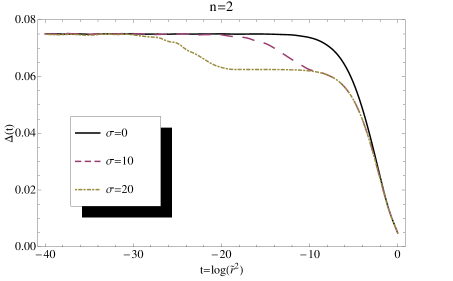
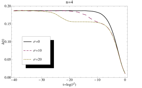
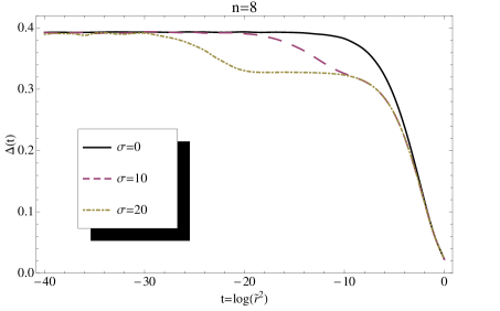
where and . This contribution, when added to (6.92) should bring the value of closer to the expected one, which is obtained by setting in (3.28). Our numerical results shown in Fig. 1 clearly demonstrate this to be the case for various values of . As the functions all approach the expected value (3.28) for or 8 and with great accuracy.
In Fig. 1 we also see that the function exhibits two finite plateaux along the renormalization group flow, which in numerical terms exactly correspond to the two particle and four particle contributions. The position at which the second plateau emerges changes as a function of , as is also illustrated in the figure. An entirely similar behaviour was found in [37] for the -function of the same model and in [51] for its effective central charge. A detailed physical interpretation has been given there.
Unfortunately, the errors on the 6 particles contribution were too large to give acceptable results.
7 Conclusions
This work has been inspired by the relationship between branch point twist fields and the ground state entanglement entropy of 1+1 dimensional integrable QFTs. This connection provides one of the main motivations to study the properties of this kind of twist field. Particularly valuable information is provided by the form factors. They can be directly employed to generate a low energy (infrared) form factor expansion of the Rényi entropy (1.4) or, as we have seen here, to extract the ultraviolet conformal dimension of the twist field. From a mathematical viewpoint one can also consider the equations (2.8)-(2.18) in their own right, investigate the properties of their solutions and try to find patterns as the particle numbers are increased.
In this paper we have constructed higher particle solutions to (2.8)-(2.18) for two particular models and have tested those solutions against the -sum rule. Our computations have revealed a number of interesting features: first, although the solution procedure and equations have many similarities with those for other local fields, it is considerably harder to find higher particle solutions for the twist field. This is mainly due to the increased number of poles the form factors have within the extended physical sheet. As a consequence, even for simple models it does not seem possible to find the nice closed determinant formulae found for example in [57, 63, 48, 49].
Second, this extra difficulty becomes particularly clear for the Ising model for which one would expect to be able to find more general results. In fact, the Ising model case suggests that solving equations (2.8)-(2.18) may not be the most effective way to construct the form factors of twist fields. In line with this, we would like to investigate whether or not other approaches, such as angular quantization [65, 66, 67] may be more suitable. In particular, the expression (2.24) found in [24] was obtained in a very natural way by the latter method.
Finally, for the RT-model we have noted that solutions to the form factors equations for branch point twist fields are generally not unique. This lack of uniqueness is not unexpected. This is because this geometric picture of the twist field as an object that connects the various sheets in a Riemann surface is not the only feature that characterizes the twist field. As its name indicates it is mainly characterized by a branch cut. One may also change the features of the twist field by putting other fields at the corresponding branch point. The expectation is that such changes will give rise to other twist fields with higher ultraviolet conformal dimensions. Our analysis of the RT-model, including the investigation of the cluster decomposition property of form factors, has revealed that some of these other twist fields correspond to non primary fields at conformal level and are likely to be related to composite fields involving the entropy-related twist field and other fields of the theory. We have found that for the RT-model and generally any model with a single particle spectrum, the most general solution for the -particle form factor of the twist field depends on free parameters. It would be very interesting to count the number of twist fields systematically by counting the number of solutions to (2.8)-(2.18). Also, we would like to investigate the conformal dimensions of all these extra fields and generally identify their counterparts at conformal level.
Concerning the numerical computations performed here, our aim has been to test the few form factor solutions obtained for two theories: the roaming trajectories model and the -homogeneous sine-Gordon model. Both share the appearance of staircase patterns for the associated effective central charges [38, 51]. For the HSG-model the same pattern has been reproduced for Zamolodchikov’s -function [55, 37] and for the conformal dimensions of certain local fields [37]. Our numerics demonstrate that such pattern is again reproduced for the conformal dimension of the twist field which exhibits two plateaux at and . For the RT-model we focused on the first and second steps in the staircase pattern only, corresponding to and , respectively.
An interesting conclusion that can be drawn from our numerics, specially for the -HSG model, is that the function given by (3.26) behaves exactly as
| (7.94) |
where is Zamolodchikov’s -function. Should this identity be exact, it would mean that the function is positive definite and monotonically decreasing (as a function of ), just as . It is however not obvious why (3.26) should have these features. Clearly, they tell us something fundamental about the nature of the correlation function and the branch point twist field. It would be very interesting to investigate this further, particularly its implications (if any) for the bi-partite entanglement entropy of integrable QFTs [68].
Acknowledgments:
The authors are grateful to Patrick Dorey, Benjamin Doyon and Andreas Fring for their feedback on this manuscript.
Appendix A Explicit formulae for and
The constants in (4.48) are given by
| (A.95) | |||||
| (A.96) | |||||
| (A.97) | |||||
| (A.98) | |||||
| (A.99) | |||||
| (A.100) | |||||
All the constants above are real for real and they remain real when , as one would expect.
The constants in (4.49) are given by
| (A.101) | |||||
| (A.102) | |||||
| (A.103) | |||||
| (A.104) | |||||
| (A.105) |
| (A.106) | |||||
| (A.107) | |||||
| (A.108) | |||||
| (A.109) | |||||
| (A.110) |
References
- [1] A. Einstein, B. Podolsky, and N. Rosen, Can quantum-mechanical description of physical reality be considered complete?, Phys. Rev. 47, 777–780 (1935).
- [2] A. Aspect, J. Dalibard, and G. Roger, Experimental test of Bell’s inequalities using time-varying analyzers, Phys. Rev. Lett. 49, 1804–1807 (1982).
- [3] M. A. Nielsen and I. L. Chuang, Quantum computation and quantum information, Cambridge University Press (2000).
- [4] C. Macchiavello, G. M. Palma, and A. Zeilinger, Quantum computation and quantum information theory, World Scientific (2000).
- [5] C. H. Bennet, H. J. Bernstein, S. Popescu, and B. Schumacher, Concentrating partial entanglement by local operations, Phys. Rev. A53, 2046–2052 (1996).
- [6] A. Osterloh, L. Amico, G. Falci, and R. Fazio, Scaling of entanglement close to a quantum phase transition, Nature 416, 608–610 (2002).
- [7] T. J. Osborne and M. A. Nielsen, Entanglement in a simple quantum phase transition, Phys. Rev. A66, 032110 (2002).
- [8] H. Barnum, E. Knill, G. Ortiz, R. Somma, and L. Viola, A subsystem-indepent generalization of entanglement, Phys. Rev. Lett. 92, 107902 (2004).
- [9] F. Verstraete, M. A. Martin-Delgado, and J. I. Cirac, Diverging entanglement length in gapped quantum spin systems, Phys. Rev. Lett. 92, 087201 (2004).
- [10] K. Audenaert, J. Eisert, M. B. Plenio, and R. F. Werner, Entanglement properties of the harmonic chain, Phys. Rev. A66, 042327 (2002).
- [11] G. Vidal, J. I. Latorre, E. Rico, and A. Kitaev, Entanglement in quantum critical phenomena, Phys. Rev. Lett. 90, 227902 (2003).
- [12] J. I. Latorre, E. Rico, and G. Vidal, Ground state entanglement in quantum spin chains, Quant. Inf. Comput. 4, 48–92 (2004).
- [13] J. I. Latorre, C. A. Lutken, E. Rico, and G. Vidal, Fine-grained entanglement loss along renormalization group flows, Phys. Rev. A71, 034301 (2005).
- [14] B.-Q. Jin and V. Korepin, Quantum spin chain, Toeplitz determinants and Fisher-Hartwig conjecture, J. Stat. Phys. 116, 79–95 (2004).
- [15] N. Lambert, C. Emary, and T. Brandes, Entanglement and the phase transition in single-mode superradiance, Phys. Rev. Lett. 92, 073602 (2004).
- [16] J. P. Keating and F. Mezzadri, Entanglement in quantum spin chains, symmetry classes of random matrices, and conformal field theory, Phys. Rev. Lett. 94, 050501 (2005).
- [17] R. A. Weston, The entanglement entropy of solvable lattice models, J. Stat. Mech. 0603, L002 (2006).
- [18] E. Ercolessi, S. Evangelisti, and F. Ravanini, Exact entanglement entropy of the XYZ model and its sine- Gordon limit, Phys. Lett. A374, 2101–2105 (2010).
- [19] E. Ercolessi, S. Evangelisti, F. Franchini, and F. Ravanini, Essential singularity in the Renyi entanglement entropy of the one-dimensional XYZ spin-1/2 chain, Phys. Rev. B83, 012402 (2011).
- [20] O. A. Castro-Alvaredo and B. Doyon, Permutation operators, entanglement entropy, and the XXZ spin chain in the limit , J. Stat. Mech. 1102, P02001 (2011).
- [21] C. Holzhey, F. Larsen, and F. Wilczek, Geometric and renormalized entropy in conformal field theory, Nucl. Phys. B424, 443–467 (1994).
- [22] P. Calabrese and J. L. Cardy, Entanglement entropy and quantum field theory, J. Stat. Mech. 0406, P002 (2004).
- [23] P. Calabrese and J. L. Cardy, Evolution of entanglement entropy in one-dimensional Systems, J. Stat. Mech. 0504, P010 (2005).
- [24] J. L. Cardy, O. A. Castro-Alvaredo, and B. Doyon, Form factors of branch-point twist fields in quantum integrable models and entanglement entropy, J. Stat. Phys. 130, 129–168 (2008).
- [25] O. A. Castro-Alvaredo and B. Doyon, Bi-partite entanglement entropy in massive 1+1-dimensional quantum field theories, J. Phys. A42, 504006 (2009).
- [26] J. Von Neumann, Mathematische Grundlagen der Quantenmechanik, Berlin, Springer Verlag (1955).
- [27] O. A. Castro-Alvaredo and B. Doyon, Bi-partite entanglement entropy in integrable models with backscattering, J. Phys. A41, 275203 (2008).
- [28] O. A. Castro-Alvaredo and B. Doyon, Bi-partite entanglement entropy in massive QFT with a boundary: the Ising model, J. Stat. Phys. 134, 105–145 (2009).
- [29] A. Rényi, Probability Theory, North-Holland, (1970).
- [30] G. Delfino, P. Simonetti, and J. L. Cardy, Asymptotic factorisation of form factors in two-dimensional quantum field theory, Phys. Lett. B387, 327–333 (1996).
- [31] P. Weisz, Exact quantum sine-Gordon soliton form-factors, Phys. Lett. B67, 179 (1977).
- [32] M. Karowski and P. Weisz, Exact S matrices and form-factors in (1+1)-dimensional field theoretic models with soliton behavior, Nucl. Phys. B139, 455–476 (1978).
- [33] F. Smirnov, Form factors in completely integrable models of quantum field theory, Adv. Series in Math. Phys. 14, World Scientific, Singapore (1992).
- [34] M. Karowski, Exact S-matrices and form-factors in (1+1)-dimensional field theoretic models with solition behaviour, Phys. Rep. 49, 229–237 (1979).
- [35] F. H. L. Essler and R. M. Konik, Applications of massive integrable quantum field theories to problems in condensed matter physics, in From Fields to Strings: Circumnavigating Theoretical Physics, edited by M. Shifman, A. Vainshtein and J. Wheater, Ian Kogan Memorial Volume, Wold Scientific (2004) .
- [36] G. Mussardo, Statistical Field Theory: An Introduction To Exactly Solved Models In Statistical Physics, Oxford University Press (2009).
- [37] O. A. Castro-Alvaredo and A. Fring, Renormalization group flow with unstable particles, Phys. Rev. D63, 021701 (2001).
- [38] A. Zamolodchikov, Resonance factorized scattering and roaming trajectories, J. Phys. A39, 12847–12861 (2006).
- [39] A. Mikhailov, M. Olshanetsky, and A. Perelomov, Two-dimensional generalized Toda lattice, Comm. Math. Phys. 79, 473–488 (1981).
- [40] A. Arinshtein, V. Fateev, and A. Zamolodchikov, Quantum S-matrix of the (1 + 1)-dimensional Toda chain, Phys. Lett. B87, 389–392 (1979).
- [41] A. B. Zamolodchikov, Thermordynamic Bethe ansatz in relativistic models. Scaling three state Potts and Lee-Yand models, Nucl. Phys. B342, 695–720 (1990).
- [42] T. R. Klassen and E. Melzer, The Thermodynamics of purely elastic scattering theories and conformal perturbation theory, Nucl. Phys. B350, 635–689 (1991).
- [43] C. Ahn, G. Delfino, and G. Mussardo, Mapping between the sinh-Gordon and Ising models, Phys. Lett. B317, 573–580 (1993).
- [44] C. Fernandez-Pousa, M. Gallas, T. Hollowood, and J. Miramontes, The symmetric space and homogeneous sine-Gordon theories, Nucl. Phys. B484, 609–630 (1997).
- [45] C. R. Fernandez-Pousa, M. V. Gallas, T. J. Hollowood, and J. L. Miramontes, Solitonic integrable perturbations of parafermionic theories, Nucl. Phys. B499, 673–689 (1997).
- [46] C. R. Fernandez-Pousa and J. L. Miramontes, Semi-classical spectrum of the homogeneous sine-Gordon theories, Nucl. Phys. B518, 745–769 (1998).
- [47] J. L. Miramontes and C. R. Fernandez-Pousa, Integrable quantum field theories with unstable particles, Phys. Lett. B472, 392–401 (2000).
- [48] O. A. Castro-Alvaredo, A. Fring, and C. Korff, Form factors of the homogeneous sine-Gordon models, Phys. Lett. B484, 167–176 (2000).
- [49] O. A. Castro-Alvaredo and A. Fring, Identifying the operator content, the homogeneous sine- Gordon models, Nucl. Phys. B604, 367–390 (2001).
- [50] O. A. Castro-Alvaredo and A. Fring, Decoupling the homogeneous sine-Gordon model, Phys. Rev. D64, 085007 (2001).
- [51] O. A. Castro-Alvaredo, A. Fring, C. Korff, and J. L. Miramontes, Thermodynamic Bethe ansatz of the homogeneous sine-Gordon models, Nucl. Phys. B575, 535–560 (2000).
- [52] O. A. Castro-Alvaredo, J. Dreissig, and A. Fring, Integrable scattering theories with unstable particles, Eur. Phys. J. C35, 393–411 (2004).
- [53] P. E. Dorey and J. L. Miramontes, Mass scales and crossover phenomena in the homogeneous sine-Gordon models, Nucl. Phys. B697, 405–461 (2004).
- [54] G. Breit and E. Wigner, Capture of slow neutrons, Phys. Rev. 49(7), 519–531 (1936).
- [55] A. B. Zamolodchikov, Irreversibility of the flux of the renormalization group in a 2-D field theory, JETP Lett. 43, 730–732 (1986).
- [56] M. Niedermaier, Varying the Unruh Temperature in Integrable Quantum Field Theories, Nucl. Phys. B535, 621–649 (1998).
- [57] A. Fring, G. Mussardo, and P. Simonetti, Form-factors for integrable Lagrangian field theories, the sinh-Gordon theory, Nucl. Phys. B393, 413–441 (1993).
- [58] T. Oota, Functional equations of form factors for diagonal scattering theories, Nucl. Phys. B466, 361–382 (1996).
- [59] O. A. Castro-Alvaredo, Form factors of boundary fields for -affine Toda field theory, J. Phys. A41, 194005 (2008).
- [60] G. Delfino and G. Niccoli, The composite operator in sinh-Gordon and a series of massive minimal models, JHEP 05, 035 (2006).
- [61] F. A. Smirnov, Reductions of the sine-Gordon model as a perturbation of minimal models of conformal field theory, Nucl. Phys. B337, 156–180 (1990).
- [62] A. B. Zamolodchikov, Two point correlation function in scaling Lee-Yang model, Nucl. Phys. B348, 619–641 (1991).
- [63] A. Koubek and G. Mussardo, On the operator content of the sinh-Gordon model, Phys. Lett. B311, 193–201 (1993).
- [64] G. Delfino, G. Mussardo, and P. Simonetti, Correlation functions along a massless flow, Phys. Rev. D51, 6620–6624 (1995).
- [65] S. L. Lukyanov and S. L. Shatashvili, Free field representation for the classical limit of quantum Affine algebra, Phys. Lett. B298, 111–115 (1993).
- [66] S. L. Lukyanov, Free field representation for massive integrable models, Commun. Math. Phys. 167, 183–226 (1995).
- [67] V. Brazhnikov and S. L. Lukyanov, Angular quantization and form factors in massive integrable models, Nucl. Phys. B512, 616–636 (1998).
- [68] O.A. Castro-Alvaredo, B. Doyon and E. Levi, in preparation.