COMET: A Recipe for Learning and Using Large Ensembles on Massive Data

Abstract

COMET is a single-pass MapReduce algorithm for learning on large-scale data. It builds multiple random forest ensembles on distributed blocks of data and merges them into a mega-ensemble. This approach is appropriate when learning from massive-scale data that is too large to fit on a single machine. To get the best accuracy, IVoting should be used instead of bagging to generate the training subset for each decision tree in the random forest. Experiments with two large datasets (5GB and 50GB compressed) show that COMET compares favorably (in both accuracy and training time) to learning on a subsample of data using a serial algorithm. Finally, we propose a new Gaussian approach for lazy ensemble evaluation which dynamically decides how many ensemble members to evaluate per data point; this can reduce evaluation cost by 100X or more.

I Introduction

The integration of computer technology into science and daily life has enabled the collection of massive volumes of data. However, this information cannot be practically analyzed on a single commodity computer because the data is too large to fit in memory. Examples of such massive-scale data include website transaction logs, credit card records, high-throughput biological assay data, sensor readings, GPS locations of cell phones, etc. Analyzing massive data requires either a) subsampling the data down to a size small enough to be processed on a workstation; b) restricting analysis to streaming methods that sequentially analyze fixed-sized subsets; or c) distributing the data across multiple computers that perform the analyses in parallel. While subsampling is a simple solution, the models it produces are often less accurate than those learned from all available data [1, 2]. Streaming methods benefit from seeing all data but typically run on a single computer, which makes processing large datasets time consuming. Distributed approaches are attractive because they can exploit multiple processors to construct models faster.

In this paper we propose to learn quickly from massive volumes of existing data using parallel computing and a divide-and-conquer approach. The data records are evenly partitioned across multiple compute nodes in a cluster, and each node independently constructs an ensemble classifier from its data partition. The resulting ensembles (from all nodes) form a mega-ensemble that votes to determine classifications. The complexities of data distribution, parallel computation, and resource scheduling are managed by the MapReduce framework [3]. In contrast to many previous uses of MapReduce to scale up machine learning that require multiple passes over the data [4, 5, 6, 7, 8, 9], this approach requires only a single pass (single MapReduce step) to construct the entire ensemble. This minimizes disk I/O and the overhead of setting up and shutting down MapReduce jobs.

Our approach is called COMET (short for Cloud Of Massive Ensemble Trees), which leverages proven learning algorithms in a novel combination. Each compute node constructs a random forest [10] based on its local data. COMET employs IVoting (importance-sampled voting) [11] instead of the usual bagging [12] to generate the training subsets used for learning the decision trees in the random forest. Chawla et al. [13] showed that IVoting produces more accurate ensembles than bagging in distributed settings. IVoting Random Forests combine the advantages of random forests (good accuracy on many problems [14, 15] and efficient learning with many features [10]) with IVoting’s ability to focus on more difficult examples. The local ensembles are combined into a mega-ensemble containing thousands of classifers in total. Using such a large ensemble is computationally expensive and overkill for data points that are easy to classify. Thus, we employ a lazy ensemble evaluation scheme that only uses as many ensemble members as are needed to make a confident prediction. We propose a new Gaussian-based approach for Lazy Ensemble Evaluation (GLEE) that is easier to implement and more scalable than previously proposed approaches.

Our main contributions are as follows:

• We present COMET, a novel MapReduce-based framework for distributed Random Forest ensemble learning. Our method uses a divide-and-conquer approach for learning on massive data and requires only a single MapReduce pass for training, unlike recent work using MapReduce to learn decision tree ensembles [7]. We also use a sampling approach called IVoting rather than the usual bagging technique.

• We develop a new approach for lazy ensemble evaluation based on a Gaussian confidence interval, called GLEE. GLEE is easier to implement and asymptotically faster to compute than the Bayesian approach proposed by Hernández-Lobato et al. [16]. Simulation experiments show that GLEE is as accurate as the Bayesian approach.

• Applying COMET to two publicly available datasets (the larger of which contains 200M examples), we demonstrate that using more data produces more accurate models than learning from a subsample on a single computational node. Our results also confirm that the IVoting sampling strategy significantly outperforms bagging in the distributed context.

II Learning on Massive Data via COMET

COMET is a recipe for large-scale distributed ensemble learning and efficient ensemble evaluation. The recipe has three components:

1. MapReduce: We write our distributed learning algorithm using MapReduce to easily parallelize the learning task. The mapper tasks build classifiers on local data partitions (“blocks” in MapReduce nomenclature), and one or more reducers can combine together and output the classifiers. The learning phase only takes a single MapReduce job. If the learned ensemble is large and/or the number of data points to be evaluated is large, evaluation can also be parallelized using at most two MapReduce jobs.

2. IVoting Random Forest: Each mapper builds an ensemble based on its local block of data (assigned by MapReduce). The mapper runs a variant of random forests that replaces bagging with IVoting (described in II-B). IVoting has the advantage that it gives more weight to difficult examples. Unlike boosting [17], however, each model in the ensemble votes with equal weight, allowing us to trivially merge the ensembles from all mappers into a single large ensemble.

3. Lazy Ensemble Evaluation: Many inputs are “easy” and the vast majority of the ensemble members agree on the classification. For these cases, querying a small sample of the members is sufficient to determine the ensemble’s prediction with high confidence. Lazy ensemble evaluation significantly lowers the prediction time for ensembles.

The rest of this section describes these three components in more detail.

II-A Exploiting MapReduce for Distributed Learning

We take a coarse-grained approach to distributed learning that minimizes communication and coordination between compute nodes. We assume that the training data is partitioned randomly into blocks in such a way that class distributions are roughly the same across all blocks. Such shuffling can be accomplished in a simple pre-processing step that maps each data item to a random block.

In the learning phase, each mapper independently learns a predictive model from an assigned data block. The learned models are aggregated together into a final ensemble model by the reducer. This is the only step that requires internode communication, and only the final models are transmitted (not the data). Thus, we only require a single MapReduce pass for training.

We implement the above strategy in the MapReduce framework [3] because the framework’s abstractions match our needs, although other parallel computing frameworks (e.g., MPI) could also be used. To use MapReduce, one loads the input data into the framework’s distributed file system and defines map and reduce functions to process key-value pair data during Map and Reduce stages, respectively. Mappers execute a map function on an assigned data block (usually read from the node’s local file system). The map function produces zero or more key-value pairs for each input; in our case, the values correspond to learned trees (with random keys). During the Reduce stage, all the pairs emitted during the Map stage are grouped by key and passed to reducer nodes that run the reduce function. The reduce function receives one key and all the associated values produced by the Map stage. Like the map function, the reduce function can emit any number of key-value pairs. Resulting pairs are written to the distributed file system. The MapReduce framework manages data partitioning, task scheduling, data replication, and restarting from failures. The reducer(s) write the learned trees to one or more output files.

The map and reduce functions for distributed ensemble learning are straightforward. The map function trains an ensemble on its local data block and then emits the learned trees. Each tree is emitted with a random key to automatically partition the ensemble across the reducers.

II-B IVoting Random Forests for Mega-Ensembles

Each mapper in COMET builds an ensemble from the local data partition using IVoting. IVoting (Importance-sampled Voting) [11] builds an ensemble by repeatedly applying the base learning algorithm (e.g., decision tree induction [18, 19]) to small samples called bites. Unlike bagging [12], examples are sampled with non-uniform probability. Suppose that $k$ IVoting iterations have been run, producing ensemble $E_{k}$ comprised of $k$ base classifiers. To form the $k+1^{\rm st}$ bite, training examples $(x,y)$ are drawn randomly. If $E_{k}$ incorrectly classifies $x$, $(x,y)$ is added to training set $B_{k+1}$. Otherwise $(x,y)$ is added to $B_{k+1}$ with probability $e(k)/(1-e(k))$, where $e(k)$ is the error rate of $E_{k}$. This process is repeated until $|B_{k+1}|$ reaches the specified bite size $b$; $b$ is typically smaller than the size of the full data. Out-of-bag (OOB) [20] predictions are used to get unbiased estimates of $e(k)$ and $E_{k}$’s accuracy on sampled points $x$. The OOB prediction for $x$ is made by voting only the ensemble members that did not see $x$ during training, i.e., $x$ was outside the base models’ training sets.

IVoting’s sequential and weighted sampling is reminiscent of boosting [17] and is similar to boosting in terms of accuracy [11]. IVoting differs from boosting in that each base model receives equal weight for deciding the ensemble’s prediction. This property simplifies merging the multiple ensembles produced by independent IVoting runs.

Breiman [11] showed that IVoting sampling generates bites containing roughly half correct and half incorrect examples. Our implementation (Algorithm 1) draws, with replacement, 50% of the bite from the examples $E_{k}$ correctly classifies and 50% from the examples $E_{k}$ incorrectly classifies (based on OOB predictions). This implementation avoids the possibility of drawing and rejecting large numbers of correct examples for ensembles with very high accuracy.

Input: Dataset $D\in(\mathcal{X},\mathcal{Y})^{*}$; Ensemble size $m$; Bite size $b\in\mathbb{N}$; Base learner $L:(\mathcal{X},\mathcal{Y})^{*}\rightarrow(\mathcal{X}\rightarrow\mathcal{Y})$

Output: Ensemble $E$

Initialize $D^{+}_{0}=D$, $D^{-}_{0}=D$, $V_{oob}[\cdot,\cdot]=0$, $E=\emptyset$;

for $i\in[1,m]$ do

       // Create the bite to train on.

       $B^{+}_{i}$ = $b/2$ uniform random samples from $D^{+}_{i-1}$;

       $B^{-}_{i}$ = $b/2$ uniform random samples from $D^{-}_{i-1}$;

       $B_{i}=B^{+}_{i}+B^{-}_{i}$;

       // Train a new ensemble member.

       $T_{i}=L(B_{i})$;

       Add $T_{i}$ to $E$;

       // Update running votes.

       for $(x_{j},y_{j})\notin B_{i}$ do

             $V_{oob}[j,T_{i}(x_{j})]$ += 1;

            

      $D^{+}_{i}=\{(x_{j},y_{j})\in D\mid y_{j}=\text{arg max}_{z}V_{oob}[j,z]\}$;

       $D^{-}_{i}=\{(x_{j},y_{j})\in D\mid y_{j}\neq\text{arg max}_{z}V_{oob}[j,z]\}$;

      

return $E$;

Algorithm 1 IVoting — Ensemble learning that samples correct & incorrect examples in equal proportions.

Any classification learning algorithm could be used for the base learner in IVoting. Our experiments use decision trees [19, 21] because they generally form accurate ensembles [22]. The trees are grown to full size (i.e., each leaf is pure or contains fewer than ten training examples) using information gain as the splitting criterion. We use full-sized trees because they generally yield slightly more accurate ensembles [22]. To increase the diversity of trees and reduce training time for data sets with large numbers of features, only a random subset of features are considered when choosing the test predicate for each tree node. This attribute subsampling is used in random forests and has been shown to improve performance and decrease training time [10]. We employ the random forest heuristic for choosing the attribute sample size $d^{\prime}=\lfloor 1+\log_{2}d\rfloor$, where $d$ is the total number of attributes.

II-C Lazy Ensemble Evaluation via a Gaussian Approach

A major drawback to large ensembles is the cost of querying all ensemble members for their predictions. In practice, many data points are easy to classify: the vast majority of the ensemble members agree on the classification. For these cases, querying a small sample of the members is sufficient to determine the ensemble’s prediction with high confidence.

We exploit this phenomena via lazy ensemble evaluation. Lazy ensemble evaluation is the strategy of only evaluating as many ensemble members as needed to make a good prediction on a case by case basis for each data point. Ensemble voting is stopped when the “lazy” prediction has high probability of being the same as the prediction from the entire ensemble. The risk that lazy evaluation stops voting too early (i.e., the probability that the early prediction is different from what the full ensemble prediction would have been) is bounded by a user-specified parameter $\alpha$. Algorithm 2 lists the lazy ensemble evaluation procedure. Let $x$ be a data point to classify using ensemble $E$, with $E$ containing $m$ base models. Initially all $m$ models are in the unqueried set $U$. In each step, a model $T$ is randomly chosen and removed from $U$ to vote on $x$; the vote is added to the running tallies of how many votes each class has received. Based on the accumulated tallies and how many ensemble members have not yet voted, the stopping criterion decides if it is safe to stop and return the classification receiving the most votes. If it is not safe, a new ensemble member is drawn, and the process is repeated until it is safe to stop or all $m$ ensemble members have been queried. Note that lazy evaluation is agnostic to whether the base models are correlated. Its goal is to approximate the (unmeasured) vote distribution from a sample of votes, and the details of the process generating the votes are irrelevant.

Input: Input $x\in\mathcal{X}$

Input: Ensemble $E$ with $m$ members of $f:\mathcal{X}\rightarrow\{1,...,c\}$

Input: $\alpha$, max. disagreement freq. for lazy vs. full eval.

Input: Vote stopping criteria $\mathrm{Stop}:(\mathbb{N}_{0}^{c},\mathbb{N}_{1},\mathbb{R}\in[0,1])\rightarrow\{\mathrm{true},\mathrm{false}\}$

Output: Approximate prediction from $E$ for input $x$.

Set $U=E$, $V=[0,...,0]$, $|V|=c$;

for $i\in[1,m]$ do

       Sample $T$ uniformly from $U$;

       Remove $T$ from $U$;

       Evaluate $v_{i}=T(x)$;

       Increment $V[v_{i}]$;

      

      if $\mathrm{Stop}(V,m,\alpha)$ then

             return $\operatorname*{arg\,max}_{i}V[i]$;

            

      

return $\operatorname*{arg\,max}_{i}V[i]$

Algorithm 2 Lazy Ensemble Evaluation

In binary categorization, the vote of each base model can be modeled as a Bernoulli random variable. Accordingly, the distribution of votes for the full ensemble is a binomial distribution with proportion parameter $p$. Provided that the number of members queried is sufficiently large, we can invoke the Central Limit Theorem and approximate the binomial distribution with a Gaussian distribution.

We propose Gaussian Lazy Ensemble Evaluation (GLEE), which uses the Gaussian distribution to infer a $(1-\alpha)$ confidence interval around the observed mean $\hat{p}$. The interval is used to test the hypothesis that the unobserved proportion of positive votes $p$ falls on the same side of 0.5 as $\hat{p}$ (and consequently, that the current estimated classification agrees with the full ensemble’s classification). If 0.5 falls outside the interval, GLEE rejects the null hypothesis that $p$ and $\hat{p}$ are on different sides of 0.5 and terminates voting early. Formally, denote the interval bounds as $\hat{p}\pm\rho\delta$, where

$$\delta =z_{\alpha/2}\frac{\sigma}{\sqrt{n}}=z_{\alpha/2}\frac{\sqrt{\hat{p}(1-\hat{p})}}{\sqrt{n}}$$

and

$$\rho =\begin{cases}\sqrt{\frac{m-n}{m-1}}&\text{ if }n>0.05m\\ 1&\text{ otherwise.}\end{cases}$$

The critical value $z_{\alpha/2}$ is the usual value from the standard normal distribution. The finite population correction (FPC) $\rho$ accounts for the fact that base models are drawn from a finite ensemble. Intuitively, uncertainty about $p$ shrinks as the set $U$ becomes small. To ensure the Gaussian approximation is reasonable, GLEE only stops evaluation only once some minimum number of models have voted. Using simulation experiments we found 15, 30, and 45 reasonable for $\alpha\geq 10^{-2}$, $\alpha=10^{-3}$, and $\alpha=10^{-4}$, respectively. (Simulation methodology is described in Section III.)

The above hypothesis test only requires the lower bound (if $\hat{p}>0.5$) or the upper bound (if $\hat{p}<0.5$). Consequently we can improve GLEE’s statistical power by computing a one-sided interval; i.e., use $z_{\alpha}$ instead of $z_{\alpha/2}$. When the GLEE stopping criteria is invoked, the leading class (the class with the most votes so far) is treated as class 1, and the runner-up class is treated as class 0. GLEE stops evaluation early if the lower bound $\hat{p}-\delta$ is greater than 0.5.

Hernández-Lobato et al. [16] present another way of deciding when to stop early using Bayesian inference. We compare to this method in Section III and refer to it as Madrid Lazy Ensemble Evaluation (MLEE). In MLEE, the distribution of vote frequencies for different classes is modeled as a multinomial distribution with a uniform Dirichlet prior. The posterior distribution of the class vote proportions is updated at each evaluation step to reflect the observed base model prediction. MLEE computes the probability that the final ensemble predicts class $c$ by combinatorially enumerating the possible prediction sequences for the as-yet unqueried ensemble members, based on the current posterior distribution. Like GLEE, ensemble evaluation stops when the probability of some class exceeds the specified confidence level or when all base models have voted. MLEE is exponential in the number of classes but is $\operatorname*{\mathrm{O}}(m^{2})$ for binary classification ($m$ ensemble members), and approximations exist to make it tractable for some multi-class problems [23].

II-D Lazy Evaluation in a Distributed Context

Large ensembles (too large to fit into memory) can make predictions on massive data (also too large to fit into memory) using lazy committee evaluation. Each input is first evaluated by a sub-committee—a random subset of the ensemble small enough to fit in memory—using a lazy evaluation rule. In most cases, the sub-committee will be able to determine the ensemble’s output with high confidence and output a decision. In the rare cases where the sub-committee cannot confidently classify the input, the input is sent to the full ensemble for evaluation.

Lazy committee evaluation requires two MapReduce jobs. In the first job each mapper randomly chooses and reads one of the $p$ ensemble partitions to be the local sub-committee and lazily evaluates the sub-committee on the mapped test data it receives; only one test input needs to be in memory at a time. If the sub-committee reaches a decision, the input’s identifier and label are written directly to the file system. Otherwise, a copy of the input is written to each of $p$ reducers by using keys $1,2,\ldots,p$. In the reduce stage, each reducer reads a different ensemble partition so that every base model votes exactly once. Reducers output the vote tallies for each input they read, keyed on the input identifier. The second job performs an identity map with reducers that sum the vote tallies for each input; reducers output the class with the most votes keyed to the input’s identifier. Combining the two sets of label outputs, from the first map and second reduce, provides a label for every input.

III Comparison of Lazy Evaluation Rules

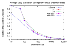
(a) Average savings from lazy evaluation when requiring 99.99% confidence that lazy prediction matches full ensemble prediction.

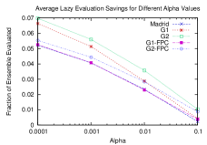
(b) Average evaluation savings for ensemble with 10K members at different confidence levels ($1-\alpha$).

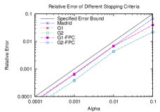
(c) Relative error of all five lazy evaluation rules is less than the specified error bound (that is, $\alpha$) for an ensemble with 10K members.

Figure 1: Lazy ensemble evaluation drastically reduces the cost of evaluating large ensembles and introduces predictable, small relative error. Graphs show five variants of lazy evaluation rules applied to simulated ensembles (see text). The rules are Madrid (MLEE), G1 (Gaussian one-tail), G2 (Gaussian two-tail), G1-FPC (G1 with finite population correction) and G2-FPC (G2 with finite population correction). All five methods provide similar speed-ups for ensembles with 500 members or more, with G1-FPC and Madrid requiring slightly fewer votes than the others. The relative errors of G1-FPC and Madrid rules are nearly identical.

This section explores the efficacy of the GLEE rule across a wide range of ensemble sizes and for varying confidence levels. We simulate votes from large ensembles to explore the rule’s behavior and to compare it to the MLEE rule.

The stopping thresholds for both methods are pre-computed and stored in a table that is indexed by the number of votes received by the leading class. One table is needed per ensemble size $m$. Pre-computing and caching the thresholds is necessary to make MLEE practical for large ensembles. Once the thresholds are computed, evaluating them requires an array lookup and comparison.

Computing the large factorials in MLEE requires care to avoid numerical overflow. Martínez-Muñoz et al. [23] suggest representing numbers in their prime factor decomposition to avoid overflow; this approach requires $\operatorname*{\mathrm{O}}(m^{3}/\log m)$ time to compute the table. We instead compute the factorials for MLEE in log-space which produces the same results and requires $\operatorname*{\mathrm{O}}(m^{2})$ total complexity. In comparison, computing the threshold table for GLEE takes $\operatorname*{\mathrm{O}}(m)$ time. This difference is significant for very large ensembles (Table I).

TABLE I: Time to Pre-compute Stopping Thresholds

	Ensemble Size
	100	1K	10K	100K	200K	1M
GLEE	1ms	1ms	3ms	12ms	17ms	57ms
MLEE	4ms	38ms	2.35s	2.76m	10.12m	3.70h

Ensemble votes are simulated as follows. A uniform random number $p\in[0,1]$ is generated to be the proportion of ensemble members that vote for class 1. The correct label for the example is 1 if $p\geq 0.5$ and 0 otherwise. Each model in the ensemble votes by sampling from a Bernoulli random variable with probability $\Pr(x=1)=p$. The ensemble is evaluated until the stopping criterion is satisfied or all $m$ ensemble members have voted. The lazy predictions under the different stopping rules and the prediction from evaluating the full ensemble are compared to the correct label to determine their relative accuracies. This process is repeated 1 million times to simulate making predictions for 1 million data points.

We report the results in terms of the average fraction of the ensemble evaluated before lazy evaluation stopped and relative error. Relative error is the relative increase in error rate from lazy evaluation (i.e., 1 - $\frac{\text{lazy accuracy}}{\text{full accuracy}}$).

Figure 1a compares five approaches to lazy ensemble evaluation. The five different approaches are Madrid (MLEE), G1 (Gaussian one-tail), G2 (Gaussian two-tail), G1-FPC (G1 with finite population correction) and G2-FPC (G2 with finite population correction). All five methods provide similar speed-ups for $m\geq 500$, with G1-FPC and Madrid requiring slightly fewer votes than the others. More importantly, we see that there is a significant benefit to applying these methods for ensembles with as few as 100 members and that the benefit becomes greater as the ensemble size grows.

In Figures 1b and 1c, we fix the ensemble size at $m=10000$ and vary $\alpha$. As one might expect, more stringent values of $\alpha$ (i.e., smaller) require evaluating more of the ensemble. Figure 1c shows that $\alpha$ upper bounds the relative error for all methods. For example, with $\alpha=0.01$ the relative error is less than 1%, and less than 3% of the ensemble needs to be evaluated by G1-FPC and MLEE. In the rest of the paper we use G1-FPC for lazy evaluation and will refer to it as the GLEE rule. Section IV presents results for GLEE on real data.

IV Experiments

To understand how well our COMET approach performs we ran a set of experiments on two large real-world datasets.

IV-A Datasets

The data sets are described in detail below; the characteristics are summarized in Table II.

IV-A1 ClueWeb09 Dataset

ClueWeb09 [24] is a web crawl of over 1 billion web pages (approximately 5TB compressed, 25TB uncompressed). For this dataset we use language categorization as the prediction task. Specifically, the task is to predict if a given web page’s language is English or non-English. The features are proportions of alpha-numeric characters ($0-9$, $a-z$, $A-Z$) plus one additional feature for any other character, for a total of 63 features.

We used MapReduce to extract features for each web page and randomly divide the data into blocks by mapping each example to a random key. Preprocessing the full ClueWeb dataset took approximately 2 hours on our Hadoop cluster and created 1000 binary files totaling approximately 259 GB and containing nearly 1B examples. From this, we randomly extracted 200M training and 1M testing examples. The training data was divided into 200 blocks, each approximately 1/4GB in size and containing 1M examples.

TABLE II: Dataset Characteristics

Name	Train	Test	Features	% Positive
ClueWeb	200M	1M	63	48.4%
eBird	1M	400K	1143	31.8%

IV-A2 eBird

The second dataset we use to evaluate COMET is the US48 eBird reference dataset [25]. Each record corresponds to a checklist collected by a bird watcher and contains counts of how many birds, broken down by species, were observed at a given location and time. In addition to the count data, each record includes attributes describing the environment in which the checklist was collected (e.g., climate, land cover), the time of year, and how much effort the observer spent. The eBird data tests how well COMET scales for problems with data having hundreds of attributes.

The prediction task in our experiment is to predict if an American Goldfinch (Carduelis tristis) will be observed at a given place and time based on the environmental and data collection attributes. We chose American Goldfinches because they are widespread throughout the United States (and thus, frequently observed) and exhibit complex migration patterns that vary from one region to another (making the prediction task hard). We used the data from 1970–2008 for training and the data from 2009 for testing. All non-zero counts were converted to 1 to create a binary prediction task. We used all attributes except meta-data attributes intended for data filtering (country, state_province, sampling_event_id, latitude, longitude, observer_id, subnational2_code).

After pre-processing, the data set contains 1.4M examples and requires 5GB of compressed storage. We subdivided the data into 14 training and 6 testing blocks. Each block contains 70K examples and requires 1/4 GB of storage.

IV-B Implementation Details

For our experiments, we used Hadoop (version 0.21), which includes MapReduce and the Hadoop distributed file system (HDFS). We used the machine learning algorithm implementations from the open-source Cognitive Foundry [26].

All experiments were run on a cluster with 65 worker nodes. Each worker node has one quad-core Intel i-720 (2.66 Ghz) processor, 12 GB of memory, four 2 TB disk drives, and 1Gb Ethernet networking. Each worker node was configured to execute up to four map or reduce tasks concurrently. To make running times directly comparable, we ran the serial algorithm on a worker node with a copy of the training data sample on the local file system.

We loaded the data into HDFS with a big enough block size to ensure each file was contained in one block (i.e., 256MB, vs. the default 64MB block size). Large block sizes improve accuracy by allowing IVoting to sample from more diverse examples.

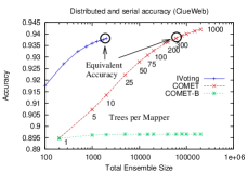
(a) Accuracy Comparison

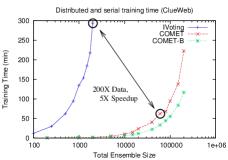
(b) Training Time Comparison

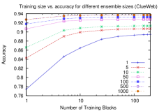
(c) Vary Training Data & Ensemble Size

Figure 2: On ClueWeb data, COMET can achieve better accuracy in less time than IVoting run serially on a subsample (IVoting line)—even though the training data size is 200M examples for COMET (distributed in 200 blocks) vs. 1M for serial IVoting. Circles denote equal accuracy. For comparison, Figures LABEL:sub@fig:clueweb-acc and LABEL:sub@fig:clueweb-time also plot the performance of a COMET variant that uses distributed bagging instead of distributed IVoting (COMET-B line). Figure LABEL:sub@fig:clueweb-data illustrates varying the number of training data blocks (1M examples per block). Different lines correspond to varying size of local ensemble. Lines for ensemble sizes 500 and 1000 are superimposed. Accuracy plateaus at approximately 40 blocks.

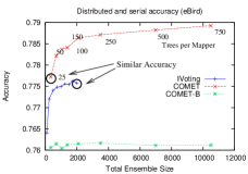
(a) Accuracy Comparison

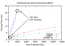
(b) Training Time Comparison

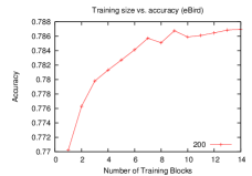
(c) Vary Training Data

Figure 3: Using 1M eBird training examples (distributed in 14 blocks), COMET is more accurate in less time than IVoting applied serially to a 70K subsample (IVoting line)—despite processing 14X more data. Circles denote similar accuracies. The COMET-B line in Figures LABEL:sub@fig:ebird-acc and LABEL:sub@fig:ebird-time shows the performance of COMET if distributed bagging is used instead of distributed IVoting. Figure LABEL:sub@fig:ebird-data illustrates varying the number of training data blocks (70K examples per block) with 200 ensemble members trained per block.

In all experiments the bite size $b$ was set to 100K for ClueWeb and 10K for eBird. These values were chosen by running IVoting for 1000 iterations on one data block with different bite sizes and measuring the accuracy on the test data. For eBird, accuracy peaked at 10K (Table III), possibly because larger bite sizes reduced the diversity of the base models. For ClueWeb, accuracy started to plateau around 100K (Table III). While larger bite sizes yielded small improvements, they also resulted in trees with big enough memory footprints to significantly limit how many ensemble members could be trained per core.

TABLE III: Accuracy for Different Bite Sizes. We used the bite size that corresponded to a leveling off of improvement, i.e., 100K for ClueWeb and 10K for eBird.

	ClueWeb	eBird
Bite Size	Accuracy	Accuracy
100	n/a	0.7265
500	n/a	0.7496
1K	0.8911	0.7614
5K	0.9089	0.7753
10K	0.9163	0.7755
50K	0.9316	0.7713
100K*	0.9359	0.7699
150K	0.9370	n/a
200K	0.9377	n/a

* eBird bite size was 70K (approx. data partition size).

In GLEE, the straightforward way to sample models (without replacement) from the ensemble is to generate a new random number for each ensemble member that is evaluated. If the cost of generating a random number is relatively expensive, lazy evaluation may not provide enough of a speed-up and may even slow down ensemble evaluation. To avoid this, our GLEE implementation permutes the ensemble order once at load time. Each ensemble evaluation is started from a different random index in this order. Thus, only a single random number is generated per ensemble prediction.

IV-C Results

We first compare COMET to subsampling (i.e., IVoting Random Forests run serially on a single block of data) to measure the benefits of learning from all data. Accuracies are computed using full ensemble evaluation (i.e., GLEE is not used).

For the ClueWeb09 data (Figure 2), the serial code trains on a single block (1M examples) using 9 different ensemble sizes: 100, 250, 500, 750, 1000, 1250, 1500, 1750, 2000. The accuracy ranges from 91.8% (100 ensemble members) up to 93.8% (2000 members). The training time ranges from 12min to 5hr. COMET trains on 200 blocks (200M examples), varying across 13 different values for the local ensemble size: 1, 5, 10, 25, 50, 75, 100, 200, 300, 400, 500, 750, 1000. The total ensemble size is 200 times the local ensemble size; thus, the largest total ensemble has 200K members. The accuracy ranges from 89.5% (corresponding to a local ensemble size of 1 and a total ensemble size of 200) to 94.2% (corresponding to a local ensemble size of 1000 and a total ensemble size of 200K) with time varying from less than 1min to 3hr, respectively. As a point of comparison, the distributed COMET model achieves an accuracy of 93.8% (the same as the best serial model) in only 60min, corresponding to a total ensemble size of 60K (300 trees per block). Thus, we achieve a 5X speed-up in training time using 200X more data without sacrificing any accuracy.

On the eBird data (Figure 3), serial IVoting trains from a single block containing 70K examples and uses the same 9 ensemble sizes as for the ClueWeb09 data. The accuracy ranges from 76.4% (for the smallest ensemble) up to 77.6% (for the largest ensemble time), and training time ranges from 1–20min. COMET trains on 14 blocks (1M examples), varying across 8 different values for the local ensemble size: 25, 50, 75, 100, 150, 250, 500, 750. The total ensemble size is 14 times the local ensemble size; thus, the largest total ensemble has 10,500 members. The accuracy ranges from 77.7% (better than the best serial accuracy) to 78.9% with time ranging from 2min to 9min. The best accuracy achieved by the serial version is 77.5% with a total ensemble size of 2000 and a training time of 21min; the distributed version improves on this with an accuracy of 77.8% for a total ensemble size of only 350 (local size of 25) and a training time of 2min. Thus, we see a 10X speed-up in training time while using 14X more data.

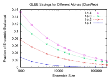
(a) ClueWeb Evaluation Savings from GLEE

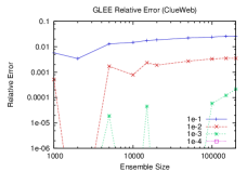
(b) ClueWeb Relative Error from GLEE

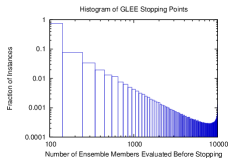
(c) Log-log histogram of GLEE early stopping points for an ensemble of size 10000 and $\alpha=0.01$ on ClueWeb data.

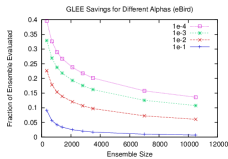
(d) eBird Evaluation Savings from GLEE

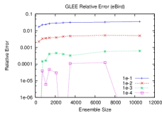
(e) eBird Relative Error from GLEE

Figure 4: For both the ClueWeb and eBird tasks, GLEE significantly reduces the average cost of ensemble evaluation while maintaining relative error below prescribed bounds. The line graphs plot GLEE (called G1-FPC in Fig. 1) using different $\alpha$ values ($1-$ confidence level). Subfigures LABEL:sub@fig:glee-clueweb-votes and LABEL:sub@fig:glee-ebird-votes show that the fraction of the ensemble evaluated decreases as ensemble size grows. In subfigures LABEL:sub@fig:glee-clueweb-err and LABEL:sub@fig:glee-ebird-err, the relative error introduced by GLEE is at most $\alpha$, the specified error rate of the approximation. The $\alpha=10^{-4}$ line in LABEL:sub@fig:glee-clueweb-err always had less than 1e-6 relative error and thus does not appear on the graph. Subfigure LABEL:sub@fig:clueweb-evr-stopping-point shows the frequency of the number of votes required. A few difficult cases require the full number of votes and are still uncertain.

Figures 2c and 3c vary the number of data blocks used in the training. For ClueWeb, all parameters are the same as above except for the following. The number of blocks is varied from 1 to 200 (with 1M examples per block), and the local ensemble size is varied from 1 to 1000. We clearly see a flattening out as the number of blocks increases, essentially flat-lining at 40. Likewise, the gain for increasing the ensemble size becomes small (invisible in this graph) for a local ensemble size of more than 250. For eBird, all parameters are the same as above except that we fix the local ensemble size at 200 and vary the number of blocks between 1 and 14. The accuracy increases almost monotonically with the number of blocks used.

Figures 2 and 3 also show the performance of COMET using bagging instead of IVoting at local nodes (COMET-B; tree construction is still randomized). While COMET-B is faster than COMET, it is less accurate than both serial and distributed IVoting (i.e., standard COMET).

The second set of experiments measures the evaluation savings and relative error incurred by using GLEE for ensembles of different sizes on the ClueWeb and eBird data (Figure 4). As expected, the results show that decreasing $\alpha$ increases the average number of votes (Figures 4a, 4d) and decreases the relative error for any size ensemble (Figures 4b, 4e). For all ensemble sizes and $\alpha$ values evaluated, using GLEE provides a significant speed-up over evaluating the entire ensemble. This speed-up increases with ensemble size, even for small values of $\alpha$. For the ClueWeb data (top row), relative error is less than 1% for $\alpha=0.01$. For an ensemble of size 1K, fewer than 8% of the ensemble needs to be evaluated, on average, and for an ensemble of size 100K, that drops to less than 1%. Similar results hold for eBird (bottom row). Thus, the cost of evaluating a large ensemble can be largely mitigated via GLEE.

Finally, Figure 4c shows a histogram of the number of evaluations needed by GLEE with $\alpha=0.01$ on a log-log scale for ClueWeb, providing insight into why the stopping method works — the vast majority of instances require evaluating only a small proportion of the ensemble. E.g., 75% of instances require 100 or fewer base model evaluations.

V Related Work

V-A Distributed Ensembles

Ensemble learning has long been used for large-scale distributed machine learning. Instead of converting a learning algorithm to be natively parallel, run the (unchanged) algorithm multiple times, in parallel, on each data partition [27, 28, 29, 13]. An aggregation strategy combines the set of learned models into an ensemble that is usually as accurate, if not more accurate, than a single model trained from all data would have been. For example, Chan and Stolfo [27] study different ways to aggregate decision tree classifiers trained from disjoint partitions. They find that voting the trees in an ensemble is sufficient if the partition size is big enough to produce accurate trees. They propose arbiter trees to intelligently combine and boost weaker trees to form accurate ensembles in spite of small partitions. Domingos [28] similarly learns sets of decision rules from partitioned data, but combines them using a simpler weighted vote. Yan et al. [30] train many randomized support vector machines with a MapReduce job; a second job runs forward stepwise selection to choose a subset with good performance. The final ensemble aggregates predictions through a simple vote. In this work we use simple voting as our aggregation strategy because our data partitions are relatively large.

Our distributed learning strategy is inspired by Chawla et al.’s work on distributed IVoting [13]. They empirically compare IVoting applied to all training data to distributed IVoting (DIVoting) in which IVoting is run independently on disjoint data partitions to create sub-ensembles that are merged to make the final ensemble. Their results show that DIVoting achieves comparable classification accuracy to (serial) IVoting with a faster running time, and better accuracy than distributed bagging that used the same sample sizes. Compared to DIVoting, COMET benefits from using MapReduce instead of MPI (for an easier implementation, scaling to data larger than the memory of all nodes, and ability to handle node failures) and incorporates lazy ensemble evaluation for efficient predictions from large ensembles. Lazy evaluation is particularly important when learning from large data sets with many data partitions. The work of Wu et al. [31] is also closely related to ours. They also train a decision tree ensemble using MapReduce in a single pass, but only train one decision tree per partition, do not use lazy ensemble evaluation, and evaluate the ensemble on a single small data set with only 699 records.

Like COMET and DIVoting, distributed boosting [32, 33] trains local ensembles from disjoint data partitions and combines them in a global ensemble. Worker nodes train boosted trees from local data but need to share learned models with each other every iteration to update the sampling weights. The resulting ensembles are at least as accurate as boosted ensembles trained serially and can be trained much faster [33]. Svore and Burges [34] experiment with a variant of distributed boosting in which only one tree is selected to add to the ensemble at each iteration. As a result the boosted ensemble grows slowly but is not as accurate as serial boosting. Chawla et al. [13] showed that DIVoting gives similar accuracy as distributed boosting without the communication overhead of sharing models.

The BagBoo algorithm [35] creates a bagged ensemble of boosted trees with each boosted sub-ensemble trained independently from data subsamples. Like COMET, BagBoo is implemented on MapReduce and creates mega-ensembles when applied to massive datasets (e.g., 1.125 million trees). The ensembles are at least as accurate as boosted ensembles. Unlike COMET, sub-ensembles are small (10–20 models) to mitigate the risk of boosting overfitting, and the non-uniform weights of trees in the ensemble precludes lazy ensemble evaluation. Because each sub-ensemble is trained from a sub-sample, a data point can appear in multiple bags (unlike COMET’s partitions); it is unclear from the algorithm description what communication cost this incurs. Since IVoting and AdaBoost yield similar accuracies [11], we expect that COMET and BagBoo would as well.

A different strategy is to distribute the computation for building a single tree; this subroutine is used to build an ensemble in which every model benefits from all training data. This approach involves multiple iterations of compute nodes calculating and sending split statistics for their local data to a controller node that chooses the best split. Most such algorithms use MPI because of the frequent communications [36, 37]. One exception is PLANET [7] which constructs decision trees from all data via multiple MapReduce passes. PLANET constructs individual trees by treating the construction of each node in the tree as a task involving the partially constructed tree. The mappers look at the examples that fall into the unexpanded tree node, collect sufficient statistics about each feature and potential split for the node, and send this information to the reducers. The reducers evaluate the best split point for each feature on a node. The controller chooses the final split point for the node based on the reducer output. Because many MapReduce jobs will be involved in building a single tree, PLANET includes many optimizations to reduce overhead, including 1) batching together node construction tasks so that each level in the tree is a single job; 2) finishing subtrees with a small number of items in-memory in the reducer; and 3) using a custom job control system to reduce job setup and teardown costs.

V-B Lazy Ensemble Evaluation

Whereas much research has studied removing unnecessary models from an ensemble (called ensemble pruning) [38], only a few studies have used lazy ensemble evaluation to dynamically speed up prediction time in proportion to the ease or difficulty of each data point. Fan et al. [29] use a Gaussian confidence interval to decide if ensemble evaluation can stop early for a test point. Their method differs from the one described in Section II-C in that a) ensemble members are always evaluated from most to least accurate, and b) confidence intervals are based on where evaluation could have reliably stopped on validation data. A fixed ordering is not necessary in our work because the base models have equal voting weight and similar accuracy; this leads to a simpler Gaussian lazy ensemble evaluation rule.

Markatopoulou et al. [39] propose a more complicated runtime ensemble pruning, where the choice of which base models to evaluate is decided by a meta-model trained to choose the most reliable models for different regions of the input data space. Their method can achieve better accuracy than using the entire ensemble, but generally will not lead to faster ensemble predictions.

VI Conclusion

COMET is a single-pass MapReduce algorithm for learning on large-scale data. It builds multiple ensembles on distributed blocks of data and merges them into a mega-ensemble. This approach is appropriate when learning from massive-scale data that is too large to fit on a single machine. It compares favorably (in both accuracy and training time) to learning on a subsample of data using a serial algorithm. Our experiments showed that it is important to use a sequential ensemble method (IVoting in our case) when building the local ensembles to get the best accuracy.

The combined mega-ensemble can be efficiently evaluated using lazy ensemble evaluation; depending on the ensemble size, the savings in evaluation cost can be 100X or better. Two options are available for lazy evaluation: our GLEE rule and the Bayesian MLEE rule [16]. GLEE is easy to implement, is asymptotically faster to compute than MLEE, and provides the same evaluation savings and approximation quality as MLEE. If one desires to further speed up evaluation or reduce the model’s storage requirements, ensemble pruning [38] could be applied to remove extraneous base models, or model compression [40] could be used to compile the ensemble into an easily deployable neural network. Ultimately the appropriateness of sacrificing some small accuracy (and how much accuracy) for faster evaluations will depend on the application domain.

In future work, it will be interesting to contrast COMET to PLANET [7], which builds trees using all available data via multiple MapReduce passes. As there is no open-source version of PLANET currently available and this procedure is highly time-consuming without special modifications to MapReduce [7], we are unable to provide direct comparisons at this time. However, we imagine that there will be some trade-off between accuracy (using all data for every tree) and time (since COMET uses only a single MapReduce pass).

Appendix A Data Preprocessing

We performed several preprocessing steps on the eBird data. First, we removed records for checklists covering $>5$ miles since most attributes are based on a checklist’s location and the location information for checklists covering large distances is less reliable. Second, count types P34 and P35 are rare in the data, so we grouped them with the semantically equivalent count types P22 and P23, respectively, by recoding P34 as P22 and P35 as P23. Third, we rederived the attributes caus_temp_avg, caus_temp_min, caus_temp_max, caus_prec, and caus_snow using the month attribute and the appropriate monthly climate features (e.g., caus_temp_avg01) to remove thousands of spurious missing values. (The eBird data providers plan to correct this processing mistake in future versions.) Fourth, missing values for categorical attributes were replaced with the special token ‘MV’. Similarly, missing and NA values for numerical attributes were recoded as -9999, a value outside the observed range of the data. With these missing value encodings, the decision tree learning algorithm can handle records with missing values as a special case if that leads to better accuracy. Fifth, we converted the categorical features (count_type, bcr, bailey_ecoregion, omernik_l3_ecoregion) into multiple binary features with one feature per valid feature value because our decision tree implementation does not yet handle categorical features.

References

- [1] C. Perlich, F. Provost, and J. S. Simonoff, “Tree induction vs. logistic regression: A learning-curve analysis,” JMLR, vol. 4, pp. 211–255, 2003.
- [2] F. Provost and V. Kolluri, “A survey of methods for scaling up inductive algorithms,” Data Mining and Knowledge Discovery, vol. 3, pp. 131–169, 1999.
- [3] J. Dean and S. Ghemawat, “MapReduce: Simplified data processing on large clusters,” Comm. ACM, vol. 51, pp. 107–113, 2008.
- [4] C.-T. Chu, S. K. Kim, Y.-A. Lin, Y. Yu, G. R. Bradski, A. Y. Ng, and K. Olukotun, “Map-Reduce for machine learning on multicore,” in NIPS 19, 2007, pp. 281–288.
- [5] E. Y. Chang, K. Zhu, H. Wang, H. Bai, J. Li, Z. Qiu, and H. Cui, “Parallelizing support vector machines on distributed computers,” in NIPS 20, 2008, pp. 257–264.
- [6] Z. Liu, H. Li, and G. Miao, “MapReduce-based backpropagation neural network over large scale mobile data,” in ICNC’10, 2010, pp. 1726–1730.
- [7] B. Panda, J. Herbach, S. Basu, and R. Bayardo, “PLANET: Massively Parallel Learning of Tree Ensembles with MapReduce,” Proc. VLDB Endowment, vol. 2, pp. 1426–1437, 2009.
- [8] J. E. Gonzalez, Y. Low, and C. Guestrin, “Residual splash for optimally parallelizing belief propagation,” in AISTATS’09, 2009, pp. 177–184.
- [9] M. Deodhar, C. Jones, and J. Ghosh, “Parallel simultaneous co-clustering and learning with map-reduce,” in IEEE Intl. Conf. on Granular Computing, 2010, pp. 149–154.
- [10] L. Breiman, “Random forests,” Machine Learning, vol. 45, pp. 5–32, 2001.
- [11] ——, “Pasting small votes for classification in large databases and on-line,” Machine Learning, vol. 36, pp. 85–103, 1999.
- [12] ——, “Bagging predictors,” Machine Learning, vol. 24, pp. 123–140, 1996.
- [13] N. V. Chawla, L. O. Hall, K. W. Bowyer, and W. P. Kegelmeyer, “Learning ensembles from bites: A scalable and accurate approach,” Journal of Machine Learning Research, vol. 5, pp. 421–451, 2004.
- [14] R. Caruana and A. Niculescu-Mizil, “An empirical comparison of supervised learning algorithms,” in ICML’06, 2006, pp. 161–168.
- [15] R. Caruana, N. Karampatziakis, and A. Yessenalina, “An empirical evaluation of supervised learning in high dimensions,” in ICML’08, 2008, pp. 96–103.
- [16] D. Hernández-Lobato, G. Martínez-Muñoz, and A. Suárez, “Statistical instance-based pruning in ensembles of independent classifiers,” IEEE Trans. Pattern Anal. Mach. Intell., vol. 31, pp. 364–369, 2009.
- [17] Y. Freund and R. E. Schapire, “Experiments with a new boosting algorithm,” in ICML’96, 1996, pp. 148–156.
- [18] L. Breiman, J. Friedman, C. J. Stone, and R. A. Olshen, Classification and Regression Trees. Chapman & Hall/CRC, 1984.
- [19] J. Quinlan, “Induction of decision trees,” Machine Learning, vol. 1, pp. 81–106, 1986.
- [20] L. Breiman, “Out-of-bag estimation,” ftp://ftp.stat.berkeley.edu/pub/users/breiman/OOBestimation.ps, 1996.
- [21] J. Quinlan, C4.5: Programs for Machine Learning. Morgan Kaufmann, 1993.
- [22] E. Bauer and R. Kohavi, “An empirical comparison of voting classification algorithms: Bagging, boosting, and variants,” Machine Learning, vol. 36, pp. 105–139, 1999.
- [23] G. Martínez-Muñoz, D. Hernández-Lobato, and A. Suárez, “Statistical instance-based ensemble pruning for multi-class problems,” in ICANN’09, 2009, pp. 90–99.
- [24] J. Callan, M. Hoy, C. Yoo, and L. Zhao, “The ClueWeb09 dataset,” http://boston.lti.cs.cmu.edu/Data/clueweb09/, 2009.
- [25] M. A. Munson, K. Webb, D. Sheldon, D. Fink, W. M. Hochachka, M. Iliff, M. Riedewald, D. Sorokina, B. Sullivan, C. Wood, and S. Kelling, The eBird Reference Dataset, Version 2.0, Cornell Lab of Ornithology and National Audubon Society, Ithaca, NY, June 2010.
- [26] J. Basilico, Z. Benz, and K. R. Dixon, “The cognitive foundry: A flexible platform for intelligent agent modeling,” in BRIMS’08, 2008, software available from http://foundry.sandia.gov/.
- [27] P. K. Chan and S. J. Stolfo, “Learning arbiter and combiner trees from partitioned data for scaling machine learning,” in KDD’95, 1995, pp. 39–44.
- [28] P. Domingos, “Using partitioning to speed up specific-to-general rule induction,” in AAAI-96 Workshop on Integrating Multiple Learned Models. Menlo Park, CA, USA: AAAI Press, 1996, pp. 29–34.
- [29] W. Fan, F. Chu, H. Wang, and P. S. Yu, “Pruning and dynamic scheduling of cost-sensitive ensembles,” in AAAI’02, 2002, pp. 146–151.
- [30] R. Yan, M.-O. Fleury, M. Merler, A. Natsev, and J. R. Smith, “Large-scale multimedia semantic concept modeling using robust subspace bagging and MapReduce,” in LS-MMRM’09, 2009, pp. 35–42.
- [31] G. Wu, H. Li, X. Hu, Y. Bi, J. Zhang, and X. Wu, “MReC4.5: C4.5 ensemble classification with MapReduce,” in ChinaGrid ’09, 2009, pp. 249–255.
- [32] C. Yu and D. Skillicorn, “Parallelizing boosting and bagging,” Queen’s University, Kingston, Canada, Tech. Rep., February 2001.
- [33] A. Lazarevic and Z. Obradovic, “Boosting algorithms for parallel and distributed learning,” Distributed and Parallel Databases, vol. 11, pp. 203–229, 2002.
- [34] K. M. Svore and C. J. Burges, “Large-scale learning to rank using boosted decision trees,” in Scaling Up Machine Learning: Parallel and Distributed Approaches. Cambridge University Press, In Press.
- [35] D. Y. Pavlov, A. Gorodilov, and C. A. Brunk, “BagBoo: A scalable hybrid bagging-the-boosting model,” in CIKM’10, 2010, pp. 1897–1900.
- [36] J. Ye, J.-H. Chow, J. Chen, and Z. Zheng, “Stochastic gradient boosted distributed decision trees,” in CIKM’09, 2009, pp. 2061–2064.
- [37] S. Tyree, K. Q. Weinberger, K. Agrawal, and J. Paykin, “Parallel boosted regression trees for web search ranking,” in WWW’11. ACM, 2011, pp. 387–396.
- [38] G. Tsoumakas, I. Partalas, and I. Vlahavas, “An ensemble pruning primer,” in Applications of Supervised and Unsupervised Ensemble Methods. Springer-Verlag, 2009, pp. 1–13.
- [39] F. Markatopoulou, G. Tsoumakas, and I. Vlahavas, “Instance-based ensemble pruning via multi-label classification,” in ICTAI’10, 2010, pp. 401–408.
- [40] C. Bucilǎ, R. Caruana, and A. Niculescu-Mizil, “Model compression,” in KDD’06, 2006, pp. 535–541.