Dressing the electromagnetic nucleon current

Abstract

A field-theory-based approach to pion photoproduction off the nucleon is used to derive a microscopically consistent formulation of the fully dressed electromagnetic nucleon current in an effective Lagrangian formalism. It is shown how the rigorous implementation of local gauge invariance at all levels of the reaction dynamics provides equations that lend themselves to practically manageable truncations of the underlying nonlinearities of the problem. The requirement of consistency also suggests a novel way of treating the pion photoproduction problem. Guided by a phenomenological implementation of gauge invariance for the truncated equations that has proved successful for pion photoproduction, an expression for the fully dressed nucleon current is given that satisfies the Ward-Takahashi identity for a fully dressed nucleon propagator as a matter of course. Possible applications include meson photo- and electroproduction processes, bremsstrahlung, Compton scattering, and $ee^{\prime}$ processes off nucleons.

I Introduction

The electromagnetic interaction provides the cleanest probe of hadronic systems available to experimentalists. Many experimental facilities, such as JLab, MAMI, ELSA, SPring-8, GRAAL, and many others around the world, therefore, use reactions employing real or virtual photons to gain information about the internal dynamics of hadronic systems. (For a recent review, see Ref. Klempt2010 .)

However, while we understand the electromagnetic interaction perfectly well at the elementary level, its applications in actual experiments do not concern elementary particles but composite systems of elementary particles that describe the internal structures of the baryonic or mesonic systems that take part in the experiments. At intermediate energies, for baryons, in particular, there usually is no need to invoke quark degrees of freedom to understand their internal structures since the internal dynamics of baryons can be described very well in terms of baryonic and mesonic degrees of freedom.

One very successful, quite fundamental way of dealing with these degrees of freedom is the effective field-theory framework of chiral perturbation theory ChPT . However, in view of its perturbative nature, this cannot be easily extended to energy regions too far away from threshold. At higher energies, one usually must rely on effective Lagrangian formulations that offer a more direct avenue to the actual meson and baryon degrees of freedom that manifest themselves in the experiments.

It is important, therefore, to understand the nature of the electromagnetic interaction with mesons and baryons in a more detailed picture. One of the most important and most basic systems in this respect is the nucleon itself.

The matrix element of the electromagnetic current operator $J^{\mu}$ of the nucleon between on-shell nucleon spinors is given by

$$\bar{u}J^{\mu}u =\bar{u}(p^{\prime})\bigg{[}e\delta_{N}\,\gamma^{\mu}+e\delta_{N}\left(\gamma^{\mu}k^{2}-k^{\mu}k\!\!\!/\right)\frac{F_{1}(k^{2})-1}{k^{2}}$$

$$\mbox{}\qquad\qquad+e\frac{i\sigma^{\mu\nu}k_{\nu}}{2m}\kappa_{N}F_{2}(k^{2})\bigg{]}u(p)~{},$$ (1)

where $e$ is the fundamental charge unit, $\delta_{N}$ is 1 or 0 for proton or neutron, respectively, and $\kappa_{N}$ is the nucleon’s anomalous magnetic moment; $m$ is the physical nucleon mass (which here is related to the incoming and outgoing nucleon four-momenta by $p^{2}=p^{\prime 2}=m^{2}$). The (scalar) Dirac and Pauli form factors, $F_{1}$ and $F_{2}$, respectively, are functions of the squared photon four-momentum $k=p^{\prime}-p$, normalized here such that $F_{1}(0)=F_{2}(0)=1$. The expression appearing within the square brackets, with two independent coefficient functions, $F_{1}$ and $F_{2}$, is the most general expression for the current $J^{\mu}$ for on-shell nucleons. As such, therefore, it appears only in physical processes involving virtual photons, like electron scattering off the nucleon, for example. While it is well known Bincer1960 that any physical mechanism involving off-shell nucleons, in general, (after having applied all available symmetry constraints) requires an expansion of the current operator in terms of six independent form factors, the simplified expression (1) nevertheless remains the current parametrization of choice for many if not most descriptions of photoprocesses within effective Lagrangian approaches irrespective of whether the photon is real or the incoming and outgoing nucleons are on-shell. A priori, of course, it is not clear how much of the dynamics of the full electromagnetic coupling to the nucleon is ignored by such a simplified approach.

It is the purpose of the present work to provide a more detailed description of the electromagnetic nucleon current $J^{\mu}$. We will start from a comprehensive field theory Haberzettl1997 that utilizes baryon and meson degrees of freedom to describe pion-nucleon scattering and that also provides — via its description of the dressed nucleon propagator — an avenue to the detailed dynamics of the nucleon’s electromagnetic interaction. The full formalism is a very complex and nonlinear Dyson-Schwinger-type approach and, as such, therefore, not easily implemented in practical applications. We will show here how this formalism can be reformulated equivalently in a manner that makes it directly amenable to physically motivated approximation schemes, thus rendering the approach practically manageable. Of decisive importance in this respect will be the fact that the internal dressing effects of the nucleon current and the dynamics of pion photoproduction are very closely related.

The paper is organized as follows. In Sec. II, concentrating on contributions due to pions, nucleons, and photons only, we introduce some basic facts needed for the description of the dressed nucleon current $J^{\mu}$. In doing so, we follow the corresponding field-theory formulation of Haberzettl Haberzettl1997 . In particular, we discuss the structure of the unique minimal current BallChiu1980 that provides the current’s Ward-Takahashi identity WTI ; WeinbergI . It is argued that the internal structure of $J^{\mu}$ is very closely related to pion photoproduction and we therefore revisit this problem in Sec. III where we extend the approach of Haberzettl, Nakayama, and Krewald Haberzettl2006 to make the truncated formalism gauge invariant in a manner that is microscopically consistent with the dressing mechanisms of the nucleon current that are provided in the subsequent Sec. IV. Finally, Sec. V provides a summarizing assessment, including a discussion of possible applications. Throughout the presentation of our formalism, we discuss possible approximations to render the complex nonlinearity of the resulting equations manageable in practice.

II Nucleon Current: Basic Considerations

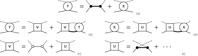
Figure 1: Generic structure of the pion-nucleon $T$ matrix employing pions and nucleons as the only hadronic degrees of freedom Haberzettl1997 . (a) Splitting of $T$ into $s$-channel pole part and non-pole $X$. (b) Bethe-Salpeter integral equation for $T$, with (c) the driving term $V$ according to Eq.(6). (d) Bethe-Salpeter integral equation for non-pole $X$, with (e) non-pole driving term $U$. Dressed vertices are solid circles; undressed ones open circles. Dressed (internal) nucleons are shown as thick lines; undressed ones as thin lines; pions are shown as dashed lines. Note that the $s$-channel pole term in the driving term $V$ is bare [because it gets dressed by the equation (b) itself] whereas, in the full theory, all mechanisms in the non-pole $U$ are fully dressed via Dyson-Schwinger-type mechanisms, as depicted in Fig. 2.

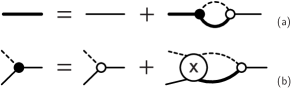
Figure 2: Dressing mechanisms for (a) the nucleon propagator $S$ and (b) the $\pi NN$ vertex $F$ according to Eq. (3) that appears in the nucleon’s self-energy contribution $\Sigma$ shown in (a) as a loop. The notation is the same as in Fig. 1.

The generic structure of the electromagnetic current $J^{\mu}$ of the nucleon can be determined in a formulation that involves pions and nucleons and photons only. Any additional hadronic degrees of freedom will only complicate the situation, but will not add any qualitatively new structure to $J^{\mu}$; in other words, they will not add anything of substance to the discussion. Using these degrees of freedom, the field-theory approach of Haberzettl Haberzettl1997 provides an expression for the current based on a Lorentz-covariant effective Lagrangian formalism. Rather than recapitulating all of the details of Ref. Haberzettl1997 , we summarize the result given there in several diagrams.

To define the dressed nucleon current $J^{\mu}$, we need the dressed nucleon propagator $S$ which is obtained from the $T$ matrix for $\pi N$ scattering. Figure 1 shows the structure of this $T$ matrix; Fig. 1(a), in particular, depicts the splitting of the full amplitude $T$ into its $s$-channel pole part and its non-pole part $X$, i.e., Haberzettl1997

$$T=\ket{F}S\bra{F}+X~{},$$ (2)

relevant for some of the present considerations. The first term here contains the nucleon propagator $S$ that provides the $s$-channel pole. The $F$s are the fully dressed $\pi NN$ vertices related to the bare vertex $f$ by

$$\ket{F}=\ket{f}+XG_{0}\ket{f}~{},$$ (3)

which is part of the nonlinear Dyson-Schwinger-type equations shown in Fig. 2. Both $T$ and $X$ are obtained as solutions of Bethe-Salpeter-type integral equations according to

$$T=V+VG_{0}T~{},$$ (4)

and

$$X=U+UG_{0}X~{},$$ (5)

as depicted in Figs. 1(b) and 1(d), respectively. The respective driving terms $V$ and $U$ differ by the bare $s$-channel diagram, as shown in Figs. 1(c) and 1(e), i.e.,

$$V=\ket{f}S_{0}\bra{f}+U~{},$$ (6)

where $S_{0}$ stands for the bare nucleon propagator. $G_{0}$ in Eqs. (3)-(5) describes the intermediate propagation of free pion and nucleon states that share the same total four-momentum of the process.

The fully dressed electromagnetic nucleon current $J^{\mu}$ derived in Ref. Haberzettl1997 is shown in Fig. 3. Formally, it results from applying the gauge-derivative procedure Haberzettl1997 to the dressed nucleon propagator $S$, however, it can be understood very simply as attaching a photon line to the propagator diagrams in Fig. 2(a) in all possible ways. To further understand the details of this structure, we mention that one of the simplest physical manifestations of the nucleon current occurs in the pion photoproduction process off the nucleon (shown in Fig. 4) because here the nucleon current provides one of the factors of the $s$-channel pole term (the other being the hadronic $\pi NN$ production vertex). It should not be surprising, therefore, that much of the detailed internal structure of the current can be understood by the same mechanisms that contribute to the pion photoproduction amplitude $M^{\mu}$. Figure 5 shows that all internal dynamics of the nucleon current $J^{\mu}$ shown in Fig. 3(a) may be represented equivalently in terms of loops over one-nucleon irreducible contributions to the pion photoproduction, with the exception of one loop involving the Kroll-Ruderman current Haberzettl1997 . This close relationship of the dressing mechanisms of the nucleon current forms the basis of the results presented below.

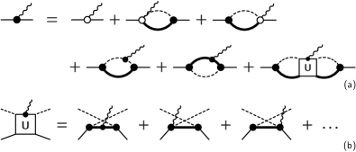
Figure 3: (a) Structure of the full electromagnetic nucleon current $J^{\mu}$ employing nucleons and pions as the only hadronic degrees of freedom Haberzettl1997 . The open circle of the first term on the right-hand side is the bare current $J^{\mu}_{0}$ and open-circle four-point functions in the next two diagrams depict the Kroll-Ruderman contact current. The last diagram subsumes the intermediate contributions of the interaction current $U^{\mu}$ arising from the photon interacting with the internal mechanisms of the one-nucleon irreducible (i.e., non-polar) $\pi N$ interaction $U$. (b) The interaction current $U^{\mu}$; explicitly shown are only the lowest-order contributions that follow from the photon interacting with the $u$-channel Born term of $\pi N$ scattering [cf. Fig. 1(e)]. The $\gamma\pi NN$ four-point vertices of the last two diagrams subsume the interaction of the photon with the interior of the fully dressed $\pi NN$ vertex (cf. last diagram in Fig. 6).

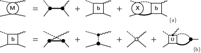
Figure 4: (a) Pion photoproduction current $M^{\mu}$ Haberzettl1997 . The diagrams show the splitting of the production current $M^{\mu}$ into the $s$-channel pole term and the remaining one-nucleon irreducible contributions, with the final-state interaction mediated by the non-pole part $X$ of the pion-nucleon $T$ matrix. (b) Structure of the Born-type contribution $b^{\mu}$, as given in Eq. (23). The four diagrams on the right-hand side depict, in the order given, the $u$- and $t$-channel contributions, the Kroll-Ruderman contact term, and the loop involving the $\pi N$ interaction current $U^{\mu}$ of Fig. 3(b).

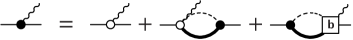
Figure 5: Alternative depiction of the nucleon current $J^{\mu}$ employing the Born-type pion-production contribution $b^{\mu}$ from Fig. 4(b).

II.1 Gauge invariance

The dressed current $J^{\mu}$ must satisfy gauge invariance; hence, it must obey the Ward-Takahashi identity (WTI) WTI ; WeinbergI ,

$$k_{\mu}J^{\mu}(p^{\prime},p)=S^{-1}(p^{\prime})Q_{N}-Q_{N}S^{-1}(p)~{},$$ (7)

where $p$ and $p^{\prime}$ are the incoming and outgoing nucleon four-momenta, respectively, and $k=p^{\prime}-p$ is the (incoming) photon momentum; $Q_{N}$ is the nucleon’s charge operator. This off-shell constraint ensures a conserved current for nucleons that are on-shell, i.e., when $p^{\prime 2}=p^{2}=m^{2}$

Without lack of generality, we may write the nucleon current as

$$J^{\mu}(p^{\prime},p)=J_{s}^{\mu}(p^{\prime},p)+T^{\mu}(p^{\prime},p)~{},$$ (8)

where $J_{s}^{\mu}$ is the minimal current that satisfies the WTI (7), i.e.,

$$k_{\mu}J_{s}^{\mu}(p^{\prime},p)=S^{-1}(p^{\prime})Q_{N}-Q_{N}S^{-1}(p)~{},$$ (9)

and $T^{\mu}$ thus is the transverse remainder, with

$$k_{\mu}T^{\mu}(p^{\prime},p)=0~{}.$$ (10)

By construction, this transversality must be manifest globally and it is not subject to any particular kinematic or dynamic restrictions.

II.2 Minimal nucleon current

Let us write the dressed propagator for a nucleon with four-momentum $p$ in a generic manner as

$$S(p)=\frac{1}{p\!\!\!/\,A(p^{2})-m\,B(p^{2})}~{},$$ (11)

where $A(p^{2})$ and $B(p^{2})$ are the two independent scalar dressing functions constrained by the residue conditions

$$A(m^{2})=B(m^{2})$$ (12a)

and

$$A(m^{2})+2m^{2}\frac{d\left[A(p^{2})-B(p^{2})\right]}{dp^{2}}\bigg{|}_{p^{2}=m^{2}}=1~{}.$$ (12b)

From the residue condition alone, one cannot in general conclude that $A(m^{2})=B(m^{2})=1$; in the structureless case, however, we have $A\equiv B\equiv 1$. (Note, however, that even though there are no explicit $p^{2}$-dependent dressing functions in the latter case, implicit dressing effects are present nevertheless owing to the fact that the mass $m$ is the physical mass.)

Following Ball and Chiu BallChiu1980 , the minimal nucleon current that satisfies the WTI (9) is given by

$$J_{s}^{\mu}(p^{\prime},p) =(p^{\prime}+p)^{\mu}\frac{S^{-1}(p^{\prime})Q_{N}-Q_{N}S^{-1}(p)}{p^{\prime 2}-p^{2}}$$

$$\mbox{}\quad+\left[\gamma^{\mu}-\frac{(p^{\prime}+p)^{\mu}}{p^{\prime 2}-p^{2}}k\!\!\!/\right]Q_{N}\frac{A(p^{\prime 2})+A(p^{2})}{2}~{}.$$ (13)

The first term here on the right-hand side is sufficient to produce the WTI, but the second part (which is transverse) is necessary to fully cancel the $1/(p^{\prime 2}-p^{2})$ singularity, as can be seen explicitly by recasting $J_{s}^{\mu}$ in the equivalent form

$$J_{s}^{\mu}(p^{\prime},p) =\gamma^{\mu}Q_{N}\frac{A(p^{\prime 2})+A(p^{2})}{2}$$

$$\quad\mbox{}+(p^{\prime}+p)^{\mu}Q_{N}\bigg{[}\frac{p\!\!\!/^{\prime}+p\!\!\!/}{2}\frac{A(p^{\prime 2})-A(p^{2})}{p^{\prime 2}-p^{2}}$$

$$\mbox{}\qquad\qquad\qquad-m\frac{B(p^{\prime 2})-B(p^{2})}{p^{\prime 2}-p^{2}}\bigg{]}~{}.$$ (14)

In fact, $J^{\mu}_{s}$ is the unique current that satisfies the WTI and also is nonsingular and symmetric in $p^{\prime}$ and $p$. Moreover, as can be seen from (14), for structureless nucleons, this reduces to the usual $\gamma^{\mu}$ Dirac current. And, invoking the generalized Gordon identity

$$(p^{\prime}+p)^{\mu}=-i\sigma^{\mu\nu}k_{\nu}+p\!\!\!/^{\prime}\gamma^{\mu}+\gamma^{\mu}p\!\!\!/~{},$$ (15)

the on-shell matrix element of $J^{\mu}_{s}$ is easily found as

$$\bar{u}J_{s}^{\mu}u =\bar{u}(p^{\prime})e\delta_{N}\bigg{\{}\gamma^{\mu}+i\frac{\sigma^{\mu\nu}k_{\nu}}{2m}\left[A(m^{2})-1\right]\bigg{\}}u(p)~{}.$$ (16)

Note that there is no $k^{2}$ dependence here, i.e., this result does not depend on whether the photon is real or virtual. This is consistent with the fact that minimal currents that satisfy the WTI as a rule cannot depend on the photon four-momentum since such a dependence always sits in transverse contributions KPS2001 . We point out in this context that the $\sigma^{\mu\nu}k_{\nu}$ contribution here must not be confused with the usual Pauli current, i.e., its coefficient is not directly related to the anomalous magnetic moment of the nucleon (which should be obvious because the entire current $J^{\mu}_{s}$ vanishes for the neutron).

Minimal current taken half on-shell

Of particular interest for many applications is to consider the half-on-shell reduction of the current. We shall do so here for an incoming on-shell nucleon interacting with a photon followed by the subsequent propagation of an off-shell nucleon, but the following considerations can be readily translated into describing the reversed situation where the outgoing nucleon is on-shell. Thus, half-on-shell, with an incoming nucleon spinor $u(p)$ on the right and an outgoing propagator $S(p+k)$ on the left, using (15), this results in

$$SJ^{\mu}_{s}u \equiv S(p+k)J^{\mu}_{s}(p+k,p)u(p)$$

$$=\left(\frac{1}{p\!\!\!/+k\!\!\!/-m}j^{\mu}_{1}+\frac{2m}{s-m^{2}}j^{\mu}_{2}\right)Q_{N}\,u(p)~{},$$ (17)

where $s=(p+k)^{2}$ and $p^{2}=m^{2}$. The (dimensionless) auxiliary currents are given by

$$j^{\mu}_{1} =\gamma^{\mu}\,\left(1-\kappa_{1}\right)+\frac{i\sigma^{\mu\nu}k_{\nu}}{2m}\kappa_{1}$$ (18a)

and

$$j^{\mu}_{2} =\frac{(2p+k)^{\mu}}{2m}\kappa_{1}+\frac{i\sigma^{\mu\nu}k_{\nu}}{2m}\kappa_{2}~{},$$ (18b)

with (dimensionless) independent coefficient functions

$$\kappa_{1} =m^{2}\frac{\left[B(s)-A(s)\right]\left[A(s)+A(m^{2})\right]}{sA^{2}(s)-m^{2}B^{2}(s)}$$ (19a)

and

$$\kappa_{2} =\frac{A(m^{2})-A(s)}{2A(s)}+\frac{A(s)+B(s)}{2A(s)}\kappa_{1}~{}.$$ (19b)

The on-shell values at $s=m^{2}$ of both coefficients are identical, i.e.,

$$\kappa_{1}(m^{2})=\kappa_{2}(m^{2})=A(m^{2})-1~{}.$$ (20)

This means they both vanish in the structureless limit, thus leaving in (17) only the usual $\gamma^{\mu}$ Dirac current together with a structureless propagator. All effects of the dressing thus reside in the terms that depend on the $\kappa_{i}$ ($i=1,2$) whose overall contributions are easily seen to be transverse.

We emphasize that Eq. (17) is exact and that it includes all possible dressing mechanisms. Its four-divergence, in particular, is given by

$$k_{\mu}\,S(p+k)J^{\mu}_{s}(p+k,p)\,u(p)=Q_{N}\,u(p)$$ (21)

and the resulting expression does not involve any dressing effects whatsoever. Any approximation, therefore, that only involves the coefficient functions $\kappa_{i}$ will have no bearing on the gauge-invariance contribution of any term containing (17). This is of direct and immediate relevance for the treatment of pion photoproduction presented in the following.

III Pion photoproduction revisited

In order to see how the gauge-invariant minimal current contribution $J^{\mu}_{s}$ of Eq. (13) can be utilized for a practically useful description of the full nucleon current $J^{\mu}$, we need to revisit the photoproduction of the pion because, as alluded to above, the internal dynamics of the current is closely related to mechanisms found in this production process, as seen in Fig. 5.

Following Ref. Haberzettl1997 , we start by writing the production current $M^{\mu}$ as

$$M^{\mu}=\ket{F}SJ^{\mu}+b^{\mu}+XG_{0}b^{\mu}$$ (22)

which is a self-evident transcription of Fig. 4(a). The first term on the right-hand side, the $s$-channel current $M^{\mu}_{s}$, contains the nucleon pole and, in the last term, $X$ provides the $\pi N$ final-state interaction (FSI) of the production current. The current $b^{\mu}$ subsuming the Born-type mechanisms may be written as

$$b^{\mu}=M^{\mu}_{u}+M^{\mu}_{t}+m^{\mu}_{\textsc{kr}}+U^{\mu}G_{0}\ket{F}$$ (23)

which describes the four terms appearing on the right-hand side of Fig. 4(b), which are, respectively, the $u$- and $t$-channel currents, the Kroll-Ruderman current Kroll1954 and the loop integration involving the $\pi N$ interaction current $U^{\mu}$ of Fig. 3(b). Generically, the overall structure of $M^{\mu}$ is presented in Fig. 6, with the first three diagrams containing the respective $s$-, $u$-, and $t$-channel pole contributions, and everything else — including the FSI contributions — being subsumed in the non-polar four-point interaction current $M^{\mu}_{\text{int}}$.

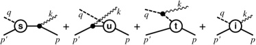
Figure 6: Generic pion photoproduction diagrams $\gamma+N\to\pi+N$, with the $s$-, $u$-, and $t$-channel pole diagrams $M^{\mu}_{s}$, $M^{\mu}_{u}$, and $M^{\mu}_{t}$, respectively, and the contact-type interaction current $M^{\mu}_{\text{int}}$ that subsumes all final-state interaction [cf. Eq. (28)]. The labels (s, u, t) at the $\pi NN$ vertices allude to the usual Mandelstam variables $s$, $u$, and $t$ that describe the respective kinematic situations. The four-momenta here are the ones used in Eqs. (30) and (45).

As discussed in Ref. Haberzettl1997 , the five-point $\pi N$ interaction current $U^{\mu}$ contains very complicated mechanisms that cannot, in general, easily be calculated exactly. Any approximations made necessary by considerations of practicality, however, need to maintain the gauge invariance of the amplitude $M^{\mu}$. The prescription put forward in Ref. Haberzettl2006 generalizes the basic procedure of Ref. Haberzettl1998 to allow the inclusion of the full FSI contribution appearing in Eq. (22) in terms of $X$. This procedure based on the generalized Ward-Takahashi identity for the production current Haberzettl1997 ; Kazes1959 is not unique, of course, since the generalized WTI does not constrain transverse current contributions. We will exploit this ambiguity here and provide an alternative gauge-invariant approximation of the amplitude $M^{\mu}$ that will turn out to be very useful in describing the mechanisms of the nucleon current $J^{\mu}$.

To this end, we split the Born current $b^{\mu}$ into its longitudinal and transverse parts,

$$b^{\mu}=b^{\mu}_{\textsc{l}}+b^{\mu}_{\textsc{t}}~{},$$ (24)

as indicated by the respective indices L and T, and write the FSI term of (22) equivalently as

$$XG_{0}b^{\mu} =XG_{0}b^{\mu}_{\textsc{l}}+XG_{0}\left[\left(M^{\mu}_{u}+M^{\mu}_{t}\right)_{\textsc{t}}+T^{\mu}_{X}\right]$$

$$\mbox{}\qquad+XG_{0}\left[\left(m^{\mu}_{\textsc{kr}}+U^{\mu}G_{0}\ket{F}\right)_{\textsc{t}}-T^{\mu}_{X}\right]~{}.$$ (25)

We have introduced here an as yet undetermined transverse current $T^{\mu}_{X}$ that cancels out in the last two terms; its choice, therefore, is of no consequence for the full formalism. Inserting this into (5), we may write

$$M^{\mu} =\ket{F}SJ^{\mu}+M^{\mu}_{u}+M^{\mu}_{t}+M^{\mu}_{c}$$

$$\mbox{}\qquad+XG_{0}\left[\big{(}M^{\mu}_{u}+M^{\mu}_{t}\big{)}_{\textsc{t}}+T^{\mu}_{X}\right]~{},$$ (26)

where

$$M^{\mu}_{c} =(1+XG_{0})\big{(}m^{\mu}_{\textsc{kr}}+U^{\mu}G_{0}\ket{F}\big{)}$$

$$\mbox{}\qquad+XG_{0}\big{(}M^{\mu}_{u}+M^{\mu}_{t}\big{)}_{\textsc{l}}-XG_{0}T_{X}^{\mu}~{}.$$ (27)

The last two terms in (26) describe the content of the interaction current (cf. the last diagram in Fig. 6), i.e.,

$$M^{\mu}_{\text{int}}=M^{\mu}_{c}+XG_{0}\left[\big{(}M^{\mu}_{u}+M^{\mu}_{t}\big{)}_{\textsc{t}}+T^{\mu}_{X}\right]~{},$$ (28)

and thus both $M^{\mu}_{\text{int}}$ and $M^{\mu}_{c}$ must obey identical constraints to render $M^{\mu}$ gauge invariant. Specifically, their four-divergences must satisfy Haberzettl1997 ; Haberzettl2006

$$k_{\mu}M^{\mu}_{\text{int}}=k_{\mu}M^{\mu}_{c}=-F_{s}e_{i}+F_{u}e_{f}+F_{t}e_{\pi}~{},$$ (29)

where $k$ is the incoming photon four-momentum and the $F_{x}$ describe the $\pi NN$ vertices (including coupling operators) in the kinematic situations corresponding to the Mandelstam variables $x=s,u,t$, as shown in Fig. 6; $e_{i}$, $e_{f}$, and $e_{\pi}$ comprise the combined isospin and charge-operator factors for the initial and final nucleons, and for the pion, respectively, of the vertices that provide charge conservation in the form $e_{i}=e_{f}+e_{\pi}$. We emphasize that the gauge-invariance condition (29) is an off-shell constraint that must always be true, i.e., it is not restricted to special kinematic or dynamic situations.

III.1 Making $M^{\mu}$ gauge invariant

The expressions for the current $J^{\mu}$ derived here are exact presuming that all contributions are calculated in the self-consistent manner prescribed by the (nonlinear) Dyson-Schwinger-type equations summarized in Figs. 1 through 5. In practice, unfortunately, this is quite out of the question in view of the enormous complexity of the nonlinear problem. Since any truncation of the full formalism is very likely to result in the violation of gauge invariance, one then needs to introduce gauge-invariance preserving (GIP) procedures to restore it. One of the big advantages of the formulation given here is that as long as the electromagnetic nucleon and pion currents satisfy their individual WTIs, any truncations necessitated by practicality can always be expressed in terms of approximations of $M^{\mu}_{c}$. And as long as these approximations are chosen to satisfy the interaction-current condition (29), gauge invariance will be preserved as a matter of course.

As discussed in Ref. Haberzettl2006 , there are various levels of sophistication at which the constraint (29) can be implemented, depending on how much of the detailed dynamics of $M^{\mu}_{c}$ can be incorporated in a particular application. For the present purpose, it is sufficient to point out that the procedures to do so are well defined and straightforward to implement.

At the simplest level, the $\pi NN$ vertices are described by phenomenological form factors, and we may then approximate all of $M^{\mu}_{c}$ by the phenomenological GIP current Haberzettl1998 ; Haberzettl2006

$$M^{\mu}_{c}\to M^{\mu}_{c} =-(1-\lambda)g\frac{\gamma_{5}\gamma^{\mu}}{2m}\tilde{F}_{t}e_{\pi}$$

$$\mbox{}\qquad-G_{\lambda}\Bigg{[}e_{i}\frac{(2p+k)^{\mu}}{s-p^{2}}\left(\tilde{F}_{s}-\hat{F}\right)$$

$$\mbox{}\qquad\qquad+e_{f}\frac{(2p^{\prime}-k)^{\mu}}{u-p^{\prime 2}}\left(\tilde{F}_{u}-\hat{F}\right)$$

$$\mbox{}\qquad\qquad+e_{\pi}\frac{(2q-k)^{\mu}}{t-q^{2}}\left(\tilde{F}_{t}-\hat{F}\right)\Bigg{]}~{},$$ (30)

where the momenta shown in Fig. 6 are being used. The first term here provides a dressed version of the Kroll-Ruderman current and the other three terms supply the gauge-invariance corrections for the $s$-, $u$, and $t$-channel contributions. The vertex functions with tilde have been stripped of their isospin factors and coupling operators, i.e., $F_{s}Q_{N}=G_{\lambda}e_{i}\tilde{F}_{s}$, etc. (see Ref. Haberzettl2006 for more technical details). The coupling operator is written as

$$G_{\lambda}=g\,\gamma_{5}\left[(1-\lambda)\frac{q\!\!\!/}{2m}+\lambda\right]~{},$$ (31)

where $g$ is the coupling strength, $q$ is the outgoing pion four-momentum, and $\lambda$ dials between pseudovector ($\lambda=0$) and pseudoscalar ($\lambda=1$) coupling. The function $\hat{F}$ must be chosen such that any one of the three terms in the square brackets remains finite if the corresponding denominators go to zero. For specific choices of how to achieve this, see Ref. Haberzettl2006 . This phenomenological expression is then non-singular and, moreover, it clearly satisfies the gauge-invariance condition (29).

The procedure to preserve gauge invariance just described is the one put forward in Ref. Haberzettl2006 , with the specific choice $T_{X}^{\mu}=0$ for the (undetermined) transverse current appearing in Eq. (26), since it has no bearing on the gauge invariance. We emphasize that the only property of the nucleon current $J^{\mu}$ itself that entered the considerations so far was the usual Ward-Takahashi identity (7) for the nucleon and its analog for the pion. In the following, we will show that taking into account the details of the internal structure of the current $J^{\mu}$ as depicted in Fig. 5 will actually suggest a different (i.e., non-zero) choice for $T^{\mu}_{X}$.

III.2 Choosing $T^{\mu}_{X}$

While the choice of the (transverse) $T^{\mu}_{X}$ is irrelevant for gauge invariance, it is clear, however, from Eq. (26), that any particular choice for $T^{\mu}_{X}$ will have a definite impact on the overall quality of the results if $M^{\mu}_{c}$ is subjected to approximations since $M^{\mu}_{c}$ itself contains $T^{\mu}_{X}$ and therefore, in general, the results will then no longer be independent of $T^{\mu}_{X}$.

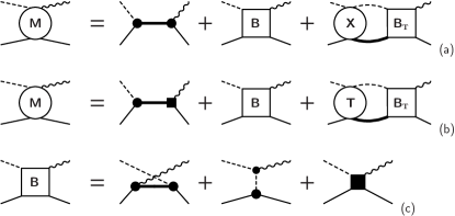
Figure 7: Representations of the photoproduction current $M^{\mu}$ (equivalent to those of Fig. 4), with (a) loop integration over the non-pole amplitude $X$ [see Eq. (33)] and (b) loop integration over the full $\pi N$ $T$ matrix [see Eq. (46)]. The details of the four-point box B are shown in (c), with the last diagram subsuming the mechanisms shown in Fig. 8. B${}_{\textsc{t}}$ denotes the restriction of B to transverse contributions. The different nucleon-current contributions appearing in the $s$-channel terms of (a) and (b) are given in Fig. 9.

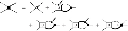
Figure 8: Diagrammatic representation of Eq. (36), with the solid square four-point vertex depicting the contact-type current $M^{\mu}_{c}$. The first two diagrams on the right-hand side show $M^{\mu}_{a}$ of Eq. (35). The indices L in the loops of the last three diagrams signify that only the longitudinal parts of the respective photon couplings are to be taken into account. These three diagrams, therefore, do not contribute for real photons.

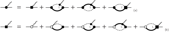
Figure 9: (a) Dressed nucleon current $J^{\mu}$ according to Eq. (42). The first term on the right-hand side (with a solid square vertex) depicts $\tilde{J}^{\mu}_{s}$ which subsumes the mechanisms shown in part (b). Diagrams labeled T or L correspond to the transverse and longitudinal contributions given in Eqs. (42) and (43), respectively. The solid-square four-point vertices in the last diagrams of each line depict $M^{\mu}_{c}$ given in Fig. 8. The phenomenological approximations discussed in Sec. IV.1 affect the (square-shaped) three- and four-point vertices of $\tilde{J}^{\mu}_{s}$ and $M^{\mu}_{c}$, respectively.

We propose here to choose the undetermined transverse current as

$$T^{\mu}_{X}=\left(M^{\mu}_{c}\right)_{\textsc{t}}~{}.$$ (32)

The photoproduction amplitude then becomes

$$M^{\mu} =\ket{F}SJ^{\mu}+M^{\mu}_{u}+M^{\mu}_{t}+M^{\mu}_{c}$$

$$\mbox{}\qquad+XG_{0}\big{(}M^{\mu}_{u}+M^{\mu}_{t}+M^{\mu}_{c}\big{)}_{\textsc{t}}~{},$$ (33)

which is shown in Fig. 7(a). $M^{\mu}_{c}$ in this expression satisfies

$$M^{\mu}_{c}+XG_{0}\left(M^{\mu}_{c}\right)_{\textsc{t}} =(1+XG_{0})M^{\mu}_{a}$$

$$\mbox{}\qquad+XG_{0}\big{(}M^{\mu}_{u}+M^{\mu}_{t}\big{)}_{\textsc{l}}~{},$$ (34)

where

$$M^{\mu}_{a}=m^{\mu}_{\textsc{kr}}+U^{\mu}G_{0}\ket{F}$$ (35)

subsumes the Kroll-Ruderman term and the loop integration over the five-point interaction current $U^{\mu}$. We may recast (34) in the form

$$M^{\mu}_{c}=M^{\mu}_{a}+UG_{0}\big{(}M^{\mu}_{u}+M^{\mu}_{t}+M^{\mu}_{c}\big{)}_{\textsc{l}}~{},$$ (36)

which is a partial integral equation in the longitudinal part of $M^{\mu}_{c}$. This equation is depicted in the diagrams of Fig. 8. We see here that the choice (32) makes the transverse parts of $M^{\mu}_{c}$ and $M^{\mu}_{a}$ identical, i.e.,

$$\left(M^{\mu}_{c}\right)_{\textsc{t}}\equiv\left(M^{\mu}_{a}\right)_{\textsc{t}}~{}.$$ (37)

Since for real photons only the transverse parts of the currents contribute to physical observables, this means that, from a practical point of view, effectively any approximation of $M^{\mu}_{c}$ is a direct approximation of $U^{\mu}G_{0}\ket{F}$, in other words, of precisely that part of the production current $M^{\mu}$ which in general cannot be calculated easily because of the complexity of its internal dynamics Haberzettl1997 . The choice (32), therefore, provides an expression for the photoproduction current, Eq. (33), that is structurally very similar to the original form (22) and one that is readily amenable to approximations. Note, in particular, that the fact that the explicit loop contribution in (33) is only transverse is irrelevant for real photons since they project out longitudinal contributions anyway, which effectively makes the structure of (33) exactly the same as (22) for such photons.

IV Dressing the Nucleon Current

Let us now turn back to the question of how to describe the dressing of the nucleon current.

According to Fig. 3(a), the dressed current may be written as Haberzettl1997

$$J^{\mu}=J^{\mu}_{\text{\tiny b}}+\bra{F}G_{0}\left(M^{\mu}_{u}+M^{\mu}_{t}+M^{\mu}_{a}\right)~{},$$ (38)

where the modified bare current $J^{\mu}_{\text{\tiny b}}$ is given by the first two diagrams on the right-hand side of Fig. 3,

$$J^{\mu}_{\text{\tiny b}}=J_{0}^{\mu}+\braket{m_{\textsc{kr}}^{\mu}}{G_{0}}{F}~{},$$ (39)

where $J_{0}^{\mu}$ is the (true) bare current and the second term is the loop containing the Kroll-Ruderman current $m_{\textsc{kr}}^{\mu}$, however, with the pion coming into the contact vertex instead of going out.

The ingredients in the last term in Eq. (38) are precisely those that enter the photoproduction amplitude and we may, therefore, use similar procedures to render them manageable in practical calculations.

Rewriting (38) equivalently in terms of $M^{\mu}_{c}$ of Eq. (27), by partially inverting the latter equation, we find

$$J^{\mu} =J^{\mu}_{\text{\tiny b}}+\bra{f}G_{0}\left[\left(M^{\mu}_{u}+M^{\mu}_{t}\right)_{\textsc{l}}+M^{\mu}_{c}-T^{\mu}_{X}\right]$$

$$\mbox{}\qquad+\bra{F}G_{0}\left[\left(M^{\mu}_{u}+M^{\mu}_{t}\right)_{\textsc{t}}+T^{\mu}_{X}\right]~{},$$ (40)

where the relationship (3) between dressed and undressed vertices, $F$ and $f$, respectively, was used. In (40), the $T^{\mu}_{X}$ dependence was left as in the original expressions to demonstrate that the choice (32) is unique in the sense that it is the only choice that produces an expression with a clear splitting of longitudinal and transverse pieces, i.e., using (32) we obtain

$$J^{\mu} =J^{\mu}_{\text{\tiny b}}+\bra{f}G_{0}\left(M^{\mu}_{u}+M^{\mu}_{t}+M^{\mu}_{c}\right)_{\textsc{l}}$$

$$\mbox{}\qquad+\bra{F}G_{0}\left(M^{\mu}_{u}+M^{\mu}_{t}+M^{\mu}_{c}\right)_{\textsc{t}}~{}.$$ (41)

For later purposes, let us write this as

$$J^{\mu}=\tilde{J}^{\mu}_{s}+\bra{F}G_{0}\left(M^{\mu}_{u}+M^{\mu}_{t}+M^{\mu}_{c}\right)_{\textsc{t}}~{},$$ (42)

where

$$\tilde{J}^{\mu}_{s}=J^{\mu}_{\text{\tiny b}}+\bra{f}G_{0}\left(M^{\mu}_{u}+M^{\mu}_{t}+M^{\mu}_{c}\right)_{\textsc{l}}~{}.$$ (43)

It is obvious, of course, that since $J^{\mu}$ and $\tilde{J}^{\mu}_{s}$ differ only by transverse pieces, their four-divergences coincide. Equations (42) and (43) are depicted in Fig. 9.

We emphasize that expression (42) for the dressed current is exact as long as we do not employ any approximations.

IV.1 Phenomenological dressing

Apart from the modified bare contribution $J^{\mu}_{\text{\tiny b}}$, the result (42) for the current provides a very suggestive even distribution of the transverse and longitudinal contributions in a loop integration over the fully dressed vertex for the former and a loop integration over the bare vertex for the latter. Being related to the bare vertices, as shown in Fig. 9(b), we would like to suggest that the longitudinal contributions to $\tilde{J}^{\mu}_{s}$ are minimal in the sense of the minimal current $J^{\mu}_{s}$ of Eq. (13), and that replacing $\tilde{J}^{\mu}_{s}$ by $J^{\mu}_{s}$ provides an excellent gauge-invariant approximation for this part of the full current. For $J^{\mu}$, instead of Eq. (42), we then write

$$J^{\mu}\to J^{\mu}=J_{s}^{\mu}+\bra{F}G_{0}\left(M^{\mu}_{u}+M^{\mu}_{t}+M^{\mu}_{c}\right)_{\textsc{t}}$$ (44)

which satisfies the usual WTI as a matter of course. Preliminary results obtained for pion photoproduction show that (44) is indeed an excellent approximation Huang2011 .

In addition, to ensure microscopic consistency among all associated reaction mechanisms, we suggest to approximate $M^{\mu}_{c}$ similar to what was discussed for photoproduction in Sec. III.1. For the present application to the nucleon current, however, we also must make sure that the current reproduces the anomalous magnetic moments for its on-shell matrix element [cf. Eq. (1)]. We, therefore, need to amend the approximation (30) according to

$$M^{\mu}_{c}\to M^{\mu}_{c} =ge\gamma_{5}\frac{i\sigma^{\mu\nu}k_{\nu}}{4m^{2}}\tilde{\kappa}_{N}-(1-\lambda)g\frac{\gamma_{5}\gamma^{\mu}}{2m}\tilde{F}_{t}e_{\pi}$$

$$\mbox{}\qquad-G_{\lambda}\Bigg{[}e_{i}\frac{(2p+k)^{\mu}}{s-p^{2}}\left(\tilde{F}_{s}-\hat{F}\right)$$

$$\mbox{}\qquad\qquad+e_{f}\frac{(2p^{\prime}-k)^{\mu}}{u-p^{\prime 2}}\left(\tilde{F}_{u}-\hat{F}\right)$$

$$\mbox{}\qquad\qquad+e_{\pi}\frac{(2q-k)^{\mu}}{t-q^{2}}\left(\tilde{F}_{t}-\hat{F}\right)\Bigg{]}~{},$$ (45)

with an additional transverse $\sigma^{\mu\nu}k_{\nu}$ current whose coefficient $\tilde{\kappa}_{N}$, in principle, needs to be fixed such that the on-shell matrix elements of the current (44) reproduce (1). The factors in this term ensure that $\tilde{\kappa}_{N}$ is dimensionless. In practice, the actual on-shell matrix elements of the nucleon current usually never enter the calculations, and one may then use $\tilde{\kappa}_{N}$ as an additional fit parameter that accounts for the current being partially off-shell. As an example of such a case, we discuss pion photoproduction in the following section.

IV.2 Application to pion photoproduction

Inserting the (exact) nucleon current (42) into the $s$-channel term of the photoproduction current (33) and using the splitting (2) of $T$ into its pole and non-pole contributions, we immediately find

$$M^{\mu} =\ket{F}S\tilde{J}_{s}^{\mu}+M^{\mu}_{u}+M^{\mu}_{t}+M^{\mu}_{c}$$

$$\mbox{}\qquad+TG_{0}\big{(}M^{\mu}_{u}+M^{\mu}_{t}+M^{\mu}_{c}\big{)}_{\textsc{t}}~{},$$ (46)

which expresses the final-state interaction in terms of the full $\pi N$ $T$ matrix instead of just its non-polar part $X$. This equation is depicted in Fig. 7(b).

This reformulation is exact if neither $\tilde{J}^{\mu}_{s}$ nor $M^{\mu}_{c}$ are approximated. In practice, however, one employs the approximations (44) and (45) to render the equations manageable. The corresponding calculations of pion photoproduction are already underway Huang2011 .

The advantage of this reformulation is twofold. First, undesirable numerical artifacts that may arise from the non-unique splitting of $T$ into its pole part and $X$ can be avoided since $T$ is closer to the actual observables than $X$. And second, and most importantly, the expression (46) only requires the half on-shell expression of $S\tilde{J}_{s}^{\mu}$ for which we can employ the result (17) when we make the approximation $\tilde{J}^{\mu}_{s}\to J^{\mu}_{s}$. In actual calculations, one may then use the two coefficient functions $\kappa_{1}$ and $\kappa_{2}$ appearing in the auxiliary currents of Eqs. (18) as fit parameters, which is an excellent approximation of the dressing effects inherent in the product $SJ_{s}^{\mu}$ when taken half on-shell. This assertion is corroborated by the preliminary numerical results of Ref. Huang2011 .

V Discussion and Summary

Based on the field-theory approach of Haberzettl Haberzettl1997 , we have presented here a formulation of the dressed electromagnetic current of the nucleon that is microscopically consistent with the reaction mechanisms inherent in meson photoproduction. The goal was to equivalently rewrite the original expressions of the full formalism in a manner that retains as much as possible of its original dynamical structure while at the same time presenting options for meaningful approximations which in practice are necessary to render the equations manageable. The consistency requirement, in particular, led to a novel approximation scheme for pion photoproduction, different from what was proposed in Ref. Haberzettl2006 . The resulting expressions are summarized diagrammatically in Fig. 7 for pion photoproduction and in Fig. 9 for the dressed nucleon current.

The full theory is exact. The guiding principle for the construction of the corresponding equations was the consistent and complete implementation of local gauge invariance at all levels of the reaction mechanisms in a manner that lends itself to transparent approximation schemes. In doing so we followed the basic strategy of Ref. Haberzettl2006 , however, with one important and essential difference. Instead of choosing the optional transverse current $T^{\mu}_{X}$ as zero, as it was done in Ref. Haberzettl2006 , we now choose it so that the resulting expression (42) for the dressed nucleon current exhibits a clean separation of transverse and longitudinal contributions that makes it straightforward to implement a phenomenological description of the dressing effects which preserves gauge invariance through the use of the minimal current $J^{\mu}_{s}$ of Eq. (13).

The phenomenological use of $J^{\mu}_{s}$ for the nucleon current makes the description of pion photoproduction particularly simple when the FSI loop of the production current $M^{\mu}$ is written in terms of the full $\pi N$ $T$ matrix (instead of with its non-pole part $X$) because the resulting $s$-channel term (17) then admits a very simple approximation by utilizing the effective dressing functions $\kappa_{1}$ and $\kappa_{2}$ as two fit parameters.

Another obvious advantage of the present scheme is that for real photons, in particular, the effective structure of the resulting photoproduction current remains very close to the full formalism even if the loops over the five-point-current contributions $U^{\mu}$ are approximated with the phenomenological contact current of Eq. (45) since for real photons the longitudinal contributions that make up the structural difference between the currents $M^{\mu}$ of Fig. 4 and of Fig. 7 are irrelevant.

The approximations discussed here in detail concern replacing the current $\tilde{J}^{\mu}_{s}$ by the minimal current $J^{\mu}_{s}$ and the contact current $M^{\mu}_{c}$ of (36) by the phenomenological GIP expression (45). It should be clear, however, that this still leaves a formidable self-consistency problem because, as can read off Fig. 9(a), the nucleon current $J^{\mu}$ also appears in one of the loops on the right-hand side. In practice, therefore, instead of solving this self-consistency problem iteratively, one might truncate it at the lowest level by employing the usual simplified on-shell expression (1) for the current in the loop.

The obvious first application of the present dressing formalism for the nucleon current is pion photoproduction, of course, since it was the consistency requirement with this process that inspired the formalism in the first place. As mentioned, this application is underway already Huang2011 , and the preliminary results obtained so far are very encouraging. In other words, the present approach is not just formally correct but the approximations suggested by its formal structure indeed lead to an excellent description of the data.

Other possible applications include any process that may benefit from a detailed microscopic description of the nucleon current. Obvious candidates are other meson production processes with both real and virtual photons off the nucleon, Compton scattering off the nucleon, and $NN$ bremsstrahlung. For virtual photons, in particular, the present formalism may also be helpful in extracting the functional behavior of electromagnetic form factors from the data.

- (1) E. Klempt and J. M. Richard, Rev. Mod. Phys. 82, 1095 (2010).
- (2) A. Pich, Rept. Prog. Phys. 58, 565 (1995); G. Ecker, Prog. Part. Nucl. Phys. 35, 1 (1995); S. Scherer, Adv. Nucl. Phys. 27, 277 (2003); V. Bernard and U.-G. Meißner, Annu. Rev. Nucl. Part. Sci. 53, 33 (2007).
- (3) J. H. Koch, V. Pascalutsa, and S. Scherer, Phys. Rev. C 65, 045202 (2002).
- (4) A. Bincer, Phys. Rev. 118, 855 (1960).
- (5) H. Haberzettl, Phys. Rev. C 56, 2041 (1997).
- (6) J. S. Ball and T.-W. Chiu, Phys. Rev. D 22, 2542 (1980).
- (7) J. C. Ward, Phys. Rev. 78, 182 (1950); Y. Takahashi, Nuovo Cimento 6, 370 (1957).
- (8) S. Weinberg, The Quantum Theory of Fields, Volume I—Foundations (Cambridge University Press, NewYork, 1995).
- (9) H. Haberzettl, K. Nakayama, and S. Krewald, Phys. Rev. C 74, 045202 (2006).
- (10) N. M. Kroll and M. A. Ruderman, Phys. Rev. 93, 233 (1954).
- (11) H. Haberzettl, C. Bennhold, T. Mart, and T. Feuster, Phys. Rev. C 58, R40 (1998).
- (12) E. Kazes, Nuovo Cimento 13, 1226 (1959).
- (13) F. Huang, M. Döring, H. Haberzettl, J. Haidenbauer, C. Hanhart, S. Krewald, U.-G. Meißner, and K. Nakayama, in preparation.