Perfect simulation for locally continuous chains of infinite order

Abstract

We establish sufficient conditions for perfect simulation of chains of infinite order on a countable alphabet. The new assumption, localized continuity, is formalized with the help of the notion of context trees, and includes the traditional continuous case, probabilistic context trees and discontinuous kernels. Since our assumptions are more refined than uniform continuity, our algorithms perfectly simulate continuous chains faster than the existing algorithms of the literature. We provide several illustrative examples.

MSC 2010 : 60G10, 62M09.

1 Introduction

The objects of this paper are stationary stochastic chains of infinite order on a countable alphabet. These chains are said to be compatible with a set of transition probabilities (depending on an unbounded portion of the past) if the later is a regular version of the conditional expectation of the former. This reflects the idea that chains of infinite order are usually determined by their conditional probabilities with respect to the past. Given a set of transition probabilities (or, simply kernels in the sequel), two natural questions are (1) existence: does there exist a stationary chain compatible with it? And (2)uniqueness: if yes, is it unique? A constructive way to answer positively these questions is to provide an algorithm based on the transition probabilities which converges a.s. and samples precisely from the stationary law of the process compatible with the given kernel. This is precisely the focus of this paper.

Perfect simulation for chains of infinite order was first done by Comets et al. (2002) under the continuity assumption. They used the fact, observed earlier by Kalikow (1990), that under this assumption, the transition probability kernel can be decomposed as a countable mixture of Markov kernels. Then, Gallo (2011) obtained a perfect simulation algorithm for chains compatible with a class of unbounded probabilistic context trees where each infinite size branch can be a discontinuity point. Both of them use an extended version of the so-called coupling from the past algorithm (CFTP in the sequel) introduced by Propp & Wilson (1996) for Markov chains. Recently, Gallo & Garcia (2010) proposed a combination between these algorithms to cover cases where the kernels are neither necessarily continuous nor necessarily probabilistic context trees. In the present paper we consider a broader class of kernels that includes all the above cases, in fact, all the results of the above cited works can be obtained as corollaries of the present work.

Other recent results in the area are the papers of Garivier (2011) and De Santis & Piccioni (2012). The former introduced an elegant CFTP algorithm which works without the weak non-nullness assumption, designed à la Propp & Wilson (1996). Their work does not intend to exhibit explicit sufficient conditions for a CFTP to be feasible and has a more algorithmic-motivated approach. The later introduced an interesting framework, making use of an a priori knowledge about the histories, extracted from the auxiliary sequence of random variables used for the simulation. Their general conditions are not explicitly given on the kernel, difficulting the comparison with our method. Notice, however, that our result is a strict generalization of Theorem 4.1 in Comets et al. (2002) whereas the regime of slow continuity rate is not present in their paper. To be more transparent, we show that all the examples of De Santis & Piccioni (2012) satisfy our conditions when considering the weakly non-null cases.

Let us emphasize also that discontinuities appear quite naturally. Section 5 present several examples. On the other hand, relaxing the continuity assumption has an interest not only from a mathematical point of view, but also from an applied point of view. Practitioners generally seek to build models which are as general as possible. From data, it is not possible to check the rate of decay of the dependence on the past, and therefore, we do not know if we have continuity.

One of the main concepts introduced in this paper is the notion of skeleton related to a transition probability kernel. It is the smallest context tree composed by the set of pasts which have a continuity rate which converges slowly to zero, or even which does not converge to zero (discontinuity points). This concept is reminiscent of the concept of bad pasts, meaning the set of discontinuous pasts for a given two-sided specification, which appears in the framework of almost-Gibbsianity in the statistical physics literature. We refer to van Enter et al. (2008) for a discussion on the subject. Almost-Gibbs measures appear in several situations, for example random walk in random scenery (see for example, den Hollander et al. (2005) and den Hollander & Steif (2006)), projection of the Ising model on a layer (Maes et al. (1999)), intermittency (Maes et al. (2000)), projection of Markov measures (Chazottes & Ugalde (2011)). From this point of view, our work exhibits a large class of almost-Gibbs measures that can be perfectly simulated.

Our first main result, Theorem 4.1, deals with locally continuous chains. Local continuity corresponds to assume that there exists a stopping time for the reversed-time process, beyond which the decay of the dependence on the past occurs uniformly. Theorem 4.1 states that, if the localized-continuity rate decays fast enough to zero, we can perfectly simulate the stationary chain by CFTP. More precisely, according to this rate, we specify several regimes for the tail distribution of the coalescence time. Theorem 7.1 presents an interesting extension where we remove the local continuity assumption. This means that this later result deals with chains such that no stopping time can tell whether or not the past we consider is a continuity point for $P$. Here also, we give explicit examples, motivating these two theorems.

It is important to emphasize that these results not only enlarge the class of processes which can be perfectly simulated but also they can be interpreted as a method to “speed up” the perfect simulation algorithm proposed by Comets et al. (2002). Assume that the kernel is such that their algorithm can be performed (that is, is continuous, with a sufficiently fast continuity rate), but with an infinite expected time, due to some pasts which slow down the continuity rate. Our method allows us to include these pasts into the set of infinite size contexts of the skeleton. Then, depending on the position of these branches (that is, depending on the form of the skeleton), our results show that the perfect simulation might be done in a finite expected time.

Our perfect simulation algorithm for the given kernel $P$ requires that the skeleton is itself perfectly simulable. However, this apparent handicap is easy to overcome. Sufficient conditions for perfect simulability can be explicitly obtained for a wide class of skeleton context trees. Several examples are presented and used throughout the paper.

It is worth mentioning that Foss & Konstantopoulos (2003) showed that the notion of perfect simulation based on a coupling from the past is closely related to the almost sure existence of “renovating event”. However, the difficulty always lies in finding such event for each specific problem. In the present case, the perfect simulation scheme provides such renovating event and gives conditions for almost sure occurrence in terms of the transition probability kernel.

The paper is organized as follows. In Section 2 we present the basic definitions, the notation, and we introduce the coupling from the past algorithm for perfect simulation in a generic way. Section 3 introduces the more specific notions of local continuity and skeletons, that are fundamental for our approach to perfect simulation. Our first main result on perfect simulation (Theorem 4.1) is presented in Section 4, together with the corollaries of existence, uniqueness and regeneration scheme which are directly inherited by the constructed stationary chain. Discussion of these results and explicit examples of application are given in Section 5. The proof of Theorem 4.1 is given in Section 6. Section 7 is dedicated to an extension of Theorem 4.1. We finish the paper with some concluding remarks in Section 8.

2 Notation and basic definitions

Let $A$ be a countable alphabet. Given two integers $m\leq n$, we denote by $a_{m}^{n}$ the string $a_{m}\ldots a_{n}$ of symbols in $A$. For any $m\leq n$, the length of the string $a_{m}^{n}$ is denoted by $|a_{m}^{n}|$ and defined by $n-m+1$. We will often use the notation $\emptyset$ which will stand for the empty string, having length $|\emptyset|=0$. For any $n\in\mathbb{Z}$, we will use the convention that $a_{n+1}^{n}=\emptyset$, and naturally $|a_{n+1}^{n}|=0$. Given two strings $v$ and $v^{\prime}$, we denote by $vv^{\prime}$ the string of length $|v|+|v^{\prime}|$ obtained by concatenating the two strings. If $v^{\prime}=\emptyset$, then $v\emptyset=\emptyset v=v$. The concatenation of strings is also extended to the case where $v=\ldots a_{-2}a_{-1}$ is a semi-infinite sequence of symbols. If $n\in\{1,2,\ldots\}$ and $v$ is a finite string of symbols in $A$, $v^{n}=v\ldots v$ is the concatenation of $n$ times the string $v$. In the case where $n=0$, $v^{0}$ is the empty string $\emptyset$. Let

$$A^{-\mathbb{N}}=A^{\{\ldots,-2,-1\}}\,\,\,\,\,\,\textrm{ and }\,\,\,\,\,\,\,A^{\star}\,=\,\bigcup_{j=0}^{+\infty}\,A^{\{-j,\dots,-1\}}\,,$$

be, respectively, the set of all infinite strings of past symbols and the set of all finite strings of past symbols. The case $j=0$ corresponds to the empty string $\emptyset$. Finally, we denote by $\underline{a}=\ldots a_{-2}a_{-1}$ the elements of $A^{-\mathbb{N}}$.

Along this paper, we will often use the letters $u$, $v$ and $w$ for (finite or infinite) strings of symbols of $A$, and the letters $i$, $j$, $k$, $l$, $m$ and $n$ for integers.

Definition 2.1

A transition probability kernel (or simply kernel in the sequel) on a countable alphabet $A$ is a function

$$\begin{array}[]{cccc}P:&A\times A^{-\mathbb{N}}&\rightarrow&[0,1]\\ &(a,\underline{a})&\mapsto&P(a|\underline{a})\end{array}$$ (1)

such that $\sum_{a\in A}P(a|\underline{a})=1$ for any $\underline{a}\in A^{-\mathbb{N}}$.

For any $a\in A$, we define

$$\alpha(a):=\inf_{\underline{z}}P(a|\underline{z})\,\,\,\textrm{and}\,\,\,\alpha_{-1}:=\sum_{a\in A}\alpha(a).$$

Definition 2.2

We say that the kernel $P$ is weakly non-null if $\alpha_{-1}>0$.

Notice that, a given kernel $P$ is Markovian of order $k$ if $P(a|\underline{a})=P(a|\underline{b})$ for any $\underline{a}$ and $\underline{b}$ such that $a_{-k}^{-1}=b_{-k}^{-1}$.

A given kernel $P$ is continuous (with respect to the product topology) at some point $\underline{a}$ if $P(a|a_{-k}^{-1}\underline{z})\rightarrow P(a|\underline{a})$ whenever $k$ diverges, for any $\underline{z}$. Continuous kernels are a natural extension of Markov kernels.

In this work we will need an equivalent definition of continuity.

Definition 2.3

We say that an infinite sequence of past symbols $\underline{b}$ is a continuity point (or past) for a given kernel $P$ if the sequence $\{\omega_{k}(\underline{b})\}_{k\geq 1}$ defined by

$$\omega_{k}(\underline{b}):=\sum_{b\in A}\inf_{\underline{z}}P(b|b_{-k}^{-1}\,\underline{z})\,,\,\,k\geq 1,$$ (2)

converges to $1$, and a discontinuity point otherwise. We say that $P$ is (uniformly) continuous if the sequence $\{\omega_{k}\}_{k\geq 1}$ defined by

$$\omega_{k}:=\inf_{b_{-k}^{-1}}\sum_{b\in A}\inf_{\underline{z}}P(b|b_{-k}^{-1}\,\underline{z})\,,\,\,k\geq 1,$$ (3)

converges to $1$, and discontinuous otherwise.

If the alphabet is finite, for instance, the set $A^{-\mathbb{N}}$ is compact and therefore, our uniform continuity is equivalent to asking that every point is continuous by the Heine-Cantor Theorem. But this is not the case in general since we are not assuming finiteness of the alphabet.

We now introduce the objects of interest of the present paper, which are the stationary chains compatible with a given kernel $P$.

Definition 2.4

A stationary stochastic chain ${\bf X}=(X_{n})_{n\in{\mathbb{Z}}}$ of law $\mu$ on $A^{\mathbb{Z}}$ is said to be compatible with a family of transition probabilities $P$ if the later is a regular version of the conditional probabilities of the former, that is

$$\mu(X_{0}=a|X_{-\infty}^{-1}=a_{-\infty}^{-1})=P(a|a_{-\infty}^{-1})$$ (4)

for every $a\in A$ and $\mu$-a.e. $a_{-\infty}^{-1}$ in $A^{-\mathbb{N}}$.

Standard questions, when we consider non-Markovian kernels, are

Q1.

Does there exist a stationary chain compatible with $P$?

Q2.

Is this chain unique?

These questions can be answered using the powerful constructing method of “perfect simulation via coupling from the past”. For a stationary stochastic chain, an algorithm of perfect simulation aims to construct finite samples distributed according to the stationary measure of the chain. Propp & Wilson (1996) introduced (in the Markovian case, that is, in the case where $P$ is a transition matrix) the coupling from the past (CFTP) algorithm. This class of algorithms uses a sequence of i.i.d. random variable ${\bf U}=\{U_{i}\}_{i\in{\mathbb{Z}}}$, uniformly distributed in $[0,1[$, to construct a sample of the stationary chain.

From now on, every chain will be constructed as a function of ${\bf U}$ and therefore, the only probability space $(\Omega,\mathcal{F},\mathbb{P})$ used in this paper is the one associated to this sequence of i.i.d. r.v.’s.

A CFTP algorithm is completely determined by the update function $F$, with which are constructed a coalescence time $\theta$ and a reconstruction function $\Phi$.

The update function $F:A^{-\mathbb{N}}\cup A^{\star}\times[0,1[\rightarrow A$ has the property that for any $\underline{a}\in A^{-\mathbb{N}}$ and for any $a\in A$, $\mathbb{P}(F(\underline{a},U_{0})=a)=P(a|\underline{a})$. Define the iterations of $F$ by

$$F_{[k,l]}(\underline{a},U_{k}^{l})=F\left(\underline{a}F_{[k,k]}(\underline{a},U_{k})F_{[k,k+1]}(\underline{a},U_{k}^{k+1})\ldots F_{[k,l-1]}(\underline{a},U_{k}^{l-1}),U_{l}\right),$$ (5)

for any $-\infty<k\leq l\leq+\infty$, where $F_{[k,k]}(\underline{a},U_{k})=F(\underline{a},U_{k})$. Based on these iterations, we define, for any window $\{m,\ldots,n\}$, $-\infty<m\leq n\leq+\infty$, its coalescence time as

$$\theta[m,n]:=\max\{j\leq m:F_{[j,n]}(\underline{a},U_{j}^{n})\,\,\,\textrm{does not depend on }\,\underline{a}\},$$ (6)

with $\theta[n]:=\theta[n,n]$. Finally, the reconstruction function of time $i$ is defined by

$$[\Phi({\bf U})]_{i}=F_{[\theta[i],i]}(\underline{a},U_{\theta[i]}^{i}).$$ (7)

Given a kernel $P$, if we can find an $F$ such that $\theta[m,n]$ is a.s. finite for any $-\infty<m\leq n<+\infty$, then, the reconstructed sample $[\Phi({\bf U})]_{i}$, $i=\theta[m,n],\ldots,n$ is distributed according to the unique stationary measure. A well-known consequence of this constructive argument is that there exists a unique stationary chain compatible with $P$, answering questions Q1 and Q2 at the same time (see Corollary 4.1 below). Observe that the choice of the function $F$ is crucial in this approach, a “bad” choice could lead to a coalescence time which is not a.s. finite or having heavy tail distribution with no finite expectation. But this choice depends on the kernel, and in particular, according to the assumptions made on the kernel, we might guarantee that there exists a $F$ for which $\theta[m,n]$ is a.s. finite. Another important observation is that, a priori, such algorithms are not practical in the sense that, at each steps, it requires that we generate all the pasts $\underline{a}$. For this reason, a particular update function based on a length function (see (22)) will be defined, allowing to decide, for some pasts $\underline{a}$ and some values of $U_{0}$, what is the value of $F(\underline{a},U_{0})$ looking only at a finite portion of $\underline{a}$.

3 Local continuity and good skeleton

Definition 3.1

• A context tree on a given alphabet $A$ is a subset of $A^{-\mathbb{N}}\cup A^{\star}$ which forms a partition of $A^{-\mathbb{N}}$ and for which if $v\in\tau$, then $uv\notin\tau$ for any $u\in A^{-\mathbb{N}}\cup A^{\star}$.

• For any context tree $\tau$, we denote by ${\vphantom{\tau}}^{<\infty}{\tau}$ the set of contexts of $\tau$ having finite lengths and by ${\vphantom{\tau}}^{\infty}{\tau}$ the remaining contexts. Clearly, these subsets form a partition of $\tau$.

• For any past $\underline{a}\in A^{-\mathbb{N}}$ we denote by $c_{\tau}(\underline{a})$ the unique element of $\tau$ which is suffix of $\underline{a}$.

For our purposes, a particular class of context trees on $A$ will be of interest.

Definition 3.2

A context tree is a skeleton context tree (or simply skeleton) if it is the smallest context tree containing the set of its infinite length contexts. We also consider $\emptyset$ to be a skeleton.

In order to illustrate this notion, let us give one simple example, on $A=\{-1,+1\}$. Let

$$\underline{\tau}:=\{1,1(-1),1(-1)(-1),1(-1)(-1)(-1),\ldots\}\cup\{-\underline{1}\}.$$ (8)

and

$$\tau_{g} := \{11,(-1)1,11(-1),(-1)1(-1),11(-1)(-1),(-1)1(-1)(-1),$$

$$\quad 11(-1)(-1)(-1),(-1)1(-1)(-1)(-1)\ldots\}\cup\{-\underline{1}\}.$$

Observe that $\underline{\tau}$ and $\tau_{g}$ are indeed context trees (i.e. satisfy the requirements of the first item of Definition 3.1). However, the only infinite length context in both trees is $-\underline{1}$, and it is easy to see that $\underline{\tau}$ is the smallest context tree having this unique infinite length context. Therefore, $\underline{\tau}$ is a skeleton whereas $\tau_{g}$ is not. We will come back several times to this skeleton along the paper.

The reason why we introduced skeletons is that they give us a nice way to formalize the notion of localized continuity, which extend the continuity assumption. In Section 5 this notion is explained by mean of examples.

Definition 3.3

A kernel $P$ belongs to the class of locally continuous kernels with respect to the skeleton $\tau$ if for any $v\in{\vphantom{\tau}}^{<\infty}{\tau}$, the sequence $\{\alpha_{k}^{v}\}_{k\geq 0}$ defined by

$$\alpha_{k}^{v}:=\inf_{a_{-k}^{-1}\in A^{k}}\sum_{a\in A}\inf_{\underline{z}}P(a|v\,a_{-k}^{-1}\,\underline{z})\,,\,\,k\geq 0$$ (10)

converges to $1$. We will denote this class by LC($\tau$). The probabilistic skeleton (p.s.) of $P$ is the pair $(\tau,p)$ where $p:=\{p(a|v)\}_{a\in A,\,v\in{\vphantom{\tau}}^{<\infty}{\tau}}$,

$$p(a|v):=\inf_{\underline{z}}P(a|v\underline{z})$$ (11)

and $p(a|v)=P(a|v)$ for any $v\in{\vphantom{\tau}}^{\infty}{\tau}$.

Some observations on the above definitions.

Observation 3.1

1. If $P$ is LC($\tau$) then, all pasts $\underline{a}$ such that $|c_{\tau}(a)|<+\infty$ are continuity point for $P$. On the other hand, we require nothing on the points $\underline{a}$ such that $|c_{\tau}(\underline{a})|=\infty$. In practice, we will see later that these will be the pasts with slow continuity rate (or even the discontinuous pasts).

2. Observe that for any fixed $v\in{\vphantom{\tau}}^{<\infty}{\tau}$, $\{p(a|v)\}_{a\in A}$ needs not to be a probability distribution on $A$.

Our first main assumption for our results will be that $P$ is a probability kernel on $A=\{1,2,\ldots\}$ being locally continuous with some p.s. $(\tau,p)$. We will furthermore require that this p.s. is “good” in a sense we explain now. We first introduce sequences of random variables which are obtained as coordinatewise functions of the sequence ${\bf U}$. The first sequence, ${\bf Y}$ is defined as follows, for any $i\in\mathbb{Z}$

$$Y_{i}=\sum_{a\in A}a.{\bf 1}\left\{\sum_{j=0}^{a-1}\alpha(j)\leq U_{i}<\sum_{j=0}^{a}\alpha(j)\right\}+\star.{\bf 1}\{U_{i}\geq\alpha_{-1}\}$$ (12)

where $\alpha(0):=0$. For any ${\bf a}=a_{-\infty}^{+\infty}\in A^{\mathbb{Z}}$, we also define the sequence of r.v.’s ${\bf Y}({\bf a})$ where for any $i\in\mathbb{Z}$,

$$Y_{i}({\bf a}):=Y_{i}.{\bf 1}\{Y_{i}\in A\}+a_{i}.{\bf 1}\{Y_{i}=\star\}.$$

Finally, we define the sequence $\{c_{\tau}^{n}\}_{n\in\mathbb{Z}}$ of maximum context length (based on ${\bf Y}$) as

$$c_{\tau}^{n}:=\sup_{{\bf a}}|c_{\tau}(Y_{-\infty}^{n}({\bf a}))|\,,\,\,\,n\in\mathbb{Z},$$ (13)

where the notation $c_{\tau}(\cdot)$ was introduced in Definition 3.1. Observe that the event $\{c_{\tau}^{n}\leq k\}$ is $\mathcal{F}(Y_{n-k+1}^{n})$-measurable.

Definition 3.4

Any time belonging to the set

$$\{i\leq m:Y_{j}\in A\,\,\,\textrm{or}\,\,\,\,c_{\tau}^{j}\leq j-i\,,\,\,\,j=i,\ldots,m\}$$ (14)

is called a good coalescence time for time $m$. We say that $(\tau,p)$ is a good probability skeleton if $\bar{\theta}[0]$, the supremum over the set (14) when $m=0$, has finite expectation.

Observation 3.2

1. Any good coalescence time is measurable with respect to $\mathcal{F}(Y_{-\infty}^{m})$ (less information than $U_{-\infty}^{m}$).

2. Assuming that $(\tau,p)$ is a good p.s. of $P$ implies that there exists a set $A(\tau)\subset A$ such that $\inf_{\underline{z}}P(a|\underline{z})>0$ for all $a\in A(\tau)$. In other words, this means that we assume weak non-nullness for $P$.

3. Observe that, under the assumption that $\tau$ is a good p.s., we have $c^{j}_{\tau}<+\infty,\mathbb{P}$-a.s. for any $j\in\mathbb{Z}$.

4 Main result and direct consequences

We will say that a non-negative sequence $\{c_{n}\}_{n\in\mathbb{N}}$ decays exponentially fast to zero if there exist a constant $D>0$ and a real number $0<d<1$ such that $c_{n}\leq Dd^{n}$ for any $n$. We say that a real-valued random variable $W$ has exponential tail if $\{\mathbb{P}(|W|\geq n)\}_{n\in\mathbb{N}}$ decays exponentially fast to zero, and summable tail if $\{\mathbb{P}(|W|\geq n)\}_{n\in\mathbb{N}}$ is summable.

For any skeleton $\tau$, let

$$N(\tau):=\{i\geq 1:\exists v\in\tau,\,|v|=i\}.$$

In the sequel, one of the main characteristics of a kernel in LC($\tau$) will be the sequence of sequences $\{\{\alpha_{k}^{i}\}_{k\geq-1}\}_{i\in N(\tau)}$, defined as

$$\alpha_{k}^{i}:=\inf_{v\in{\vphantom{\tau}}^{\leq i}{\tau}}\alpha_{k}^{v},$$ (15)

where ${\vphantom{\tau}}^{\leq i}{\tau}$ denotes the set of contexts in $\tau$ having length smaller or equal to $i$. Observe that there is a notational similarity between the case where the exponent is an integer $i$ and the case where it is an element $v$ of $\tau$.

Theorem 4.1

Consider a kernel $P$ belonging to LC($\tau$) and assume that its probabilistic skeleton $(\tau,p)$ is good with good coalescence times $\bar{\theta}[0]$ for time $0$. Let $A_{0}:=\alpha_{-1}$ and for any $k\geq 1$, denote

$$A_{k}:=\left\{1-(\mathbb{E}|\bar{\theta}[0]|+1)\mathbb{P}(U_{0}>\alpha_{k}^{c_{\tau}^{-1}})\right\}\vee\alpha_{-1}.$$

Then, we can construct for $P$, an update function $F$ and a corresponding coalescence time $\theta$ such that

1. If $\sum_{k\geq 1}\prod_{j=0}^{k-1}A_{k}=+\infty$, then $\theta[0]$ is $\mathbb{P}$-a.s. finite.

2. If $\sum_{k\geq 0}(1-A_{k})<+\infty$, then $\theta[0]$ has summable tail.

3. If $\bar{\theta}[0]$ has exponential tail and $\{1-A_{k}\}_{k\geq 0}$ decays exponentially fast to zero, then $\theta[0]$ has exponential tail.

In particular, in each of these regimes, the CFTP with update function $F$ is feasible.

The proof of this result is given in Section 6. Section 5 will discuss explicit examples. We now state some direct consequences of Theorem 4.1.

Theorem 4.1 states, in particular, that the CFTP algorithm is feasible with some function $F$ (which will be constructed in the proof). We recall that this means that the algorithm constructs, for any $i\in\mathbb{Z}$, an almost surely finite sample $[\Phi({\bf U})]_{\theta[i]}^{i}$, which is a deterministic function of ${\bf U}$. In the sequel, we will often write $X_{i}$ for $[\Phi({\bf U})]_{i}$ (and ${\bf X}$ for $[\Phi({\bf U})]_{-\infty}^{+\infty}$) in order to avoid overloaded notations, keeping in mind the fact that for any $i$, $X_{i}$ is constructed as a deterministic function of ${\bf U}$. Actually, by Theorem 4.1, $X_{i}$ depends only on a $\mathbb{P}$-a.s. finite part of this sequence since $X_{i}:=[X(\ldots,u_{\theta[i]-1},U_{\theta[i]},\ldots,U_{i},u_{i+1},\ldots)]_{i}$ for any ${\bf u}\in[0,1[^{\mathbb{Z}}$. As we already mentioned in Section 2, the existence of a perfect simulation algorithm has important consequences, stated in the two next corollaries, and whose proofs use standard arguments given, for example, in Comets et al. (2002).

Corollary 4.1

(Existence and uniqueness). ${\bf X}$ is stationary and compatible with $P$. Denoting by $\mu$ the stationary measure of ${\bf X}$ we have

$$\mu(\cdot):=\mathbb{P}(\Phi({\bf U})\in\cdot).$$

Moreover, $\mu$ has support on the set of continuous pasts of $P$.

When $\mathbb{E}|\theta[0]|<+\infty$, the chain ${\bf X}$ exhibits a regeneration scheme. We call time $t$ a regeneration time for the chain ${\bf X}$ if $\theta[t,+\infty]=t$. Define the chain $\boldsymbol{\mathcal{T}}$ on $\{0,1\}$ by $\mathcal{T}_{j}:={\bf 1}\left\{j=\theta[j,+\infty]\right\}$. Then, consider the sequence of time indexes ${\bf T}$ defined by $\mathcal{T}_{j}=1$ if and only if $j=T_{l}$ for some $l$ in $\mathbb{Z}$, $T_{l}<T_{l+1}$ and with the convention $T_{0}\leq 0<T_{1}$. We say that ${\bf X}$ has a regeneration scheme if $\boldsymbol{\mathcal{T}}$ is a renewal chain (that is, if the increments $(T_{i+1}-T_{i})_{i\in\mathbb{Z}}$ are independent, and are identically distributed for $i\neq 0$).

Corollary 4.2

(Regeneration scheme). Under conditions (ii) and (iii) of Theorem 4.1, the chain ${\bf X}$ has a regeneration scheme. The random strings
$(\Phi({\bf U})_{T_{i}},\ldots,\Phi({\bf U})_{T_{i+1}-1})_{i\neq 0}$ are i.i.d. and have finite expected size. Under the stronger requirement of (iii), the lengths of these strings have exponential tail.

In words, this corollary states that the unique stationary chain compatible with $(\tau,p)$ under the conditions of Theorem 4.1 can be viewed as an i.i.d. concatenation of strings of symbols of $A$ having finite expected size. A similar result has been first obtained in Lalley (1986) for one dimensional Gibbs states under appropriate conditions on the continuity rate, and then in Comets et al. (2002) under weaker conditions. Our result strengthen all these results, and in particular, since continuity is not assumed here, our chains are not even necessarily Gibbsian. This lack of Gibbsianity is easy to establish, using the recent result of Fernández et al. (2011), in which it has been shown that the unique stationary chain compatible with the p.s. $(\underline{\tau},p)$ ($\underline{\tau}$ is the tree corresponding to a regeneration process) is not always Gibbsian, even when it satisfies continuity and $\alpha(a)>0$ for all $a\in A$.

5 Applications

In Section 5.1 we will explain how Theorem 4.1 reads in two special cases of local continuity which are the strong local continuity and the uniform local continuity. Then, we will present several examples that illustrate our results: in Section 5.2 we consider local continuity with respect to two special cases of skeletons and finally, Section 5.3 is dedicated to explicit examples.

5.1 Specific local continuities

Uniform local continuity.

Definition 5.1

A kernel $P$ belongs to the class of uniformly local continuous kernels with respect to the skeleton $\tau$ if

$$\alpha_{i}:=\inf_{v\in{\vphantom{\tau}}^{<\infty}{\tau}}\alpha_{i}^{v}\stackrel{{\scriptstyle i\rightarrow+\infty}}{{\longrightarrow}}1.$$ (16)

We will denote this class by ULC($\tau$).

When $P$ belongs to ULC($\tau$), we can use the facts that $\alpha_{i}:=\inf_{k\in N(\tau)}\alpha^{k}_{i}$ converges to $1$, and that $U_{0}$ is independent of $c^{-1}_{\tau}$ (since this later is $\mathcal{F}(U_{-\infty}^{-1})$-measurable) to obtain

$$\mathbb{P}(U_{0}\geq\alpha_{i}^{c_{\tau}^{-1}}) =\sum_{k\in N(\tau)}\mathbb{P}(U_{0}\geq\alpha_{i}^{k})\mathbb{P}(c_{\tau}^{-1}=k)\leq\mathbb{P}(U_{0}\geq\alpha_{i})\sum_{k\in N(\tau)}\mathbb{P}(c_{\tau}^{-1}=k)\leq(1-\alpha_{i}).$$ (17)

We have therefore proved the following corollary.

Corollary 5.1

Restricting the assumptions of Theorem 4.1 to the case of ULC($\tau$) kernels, the same statements hold substituting $A_{m}$ by $1-\mathbb{E}(|\bar{\theta}[0]|+1)(1-\alpha_{m})$, for any $m\geq 1$.

As we will explain in Section 5.2, Theorem 4.1 in Comets et al. (2002) and Theorem 1 in Gallo & Garcia (2010) are particular cases of uniform local continuity where $\tau=\emptyset$ and $\tau$ has a terminal string (see Definition 5.3), respectively.

Explicit examples of this regime are given by Examples 5.1, 5.2 and 5.4.

Strong local continuity.

Definition 5.2

A kernel $P$ belongs to the class of strongly local continuous kernels with respect to the skeleton $\tau$ if for any $v\in{\vphantom{\tau}}^{<\infty}{\tau}$, there exists a positive integer $h(v)$ such that for any $k\geq h(v)$, $\alpha_{k}^{v}=1$. We will denote this class by SLC($\tau$).

These kernels belong to a particular class of probability kernels known in the literature under the name of probabilistic context trees, which have been introduced by Rissanen (1983).

When $P$ belongs to SLC($\tau$) on a finite alphabet, we can use the fact that for any $i\in N(\tau)$, $\alpha_{k}^{i}=1$ for any $k\geq h(i)$, where $h(i):=\sup_{v\in{\vphantom{\tau}}^{\leq i}{\tau}}h(v)$, and we obtain, using $h^{-1}(i):=\inf\{k\geq 1:h(k)>i\}$,

$$\mathbb{P}(U_{0}\geq\alpha_{i}^{c_{\tau}^{-1}})\leq\mathbb{P}(c_{\tau}^{-1}>h^{-1}(i))=\mathbb{P}(c_{\tau}^{0}>h^{-1}(i)).$$ (18)

We have therefore proved the following corollary.

Corollary 5.2

Restricting the assumptions of Theorem 4.1 to the case of SLC($\tau$) kernels on finite alphabet, the same statements hold substituting $A_{m}$ by $1-\mathbb{E}(|\bar{\theta}[0]|+1)\mathbb{P}(c_{\tau}^{0}>h^{-1}(m))$, for any $m\geq 1$.

As we will explain in Section 5.2, the results of Gallo (2011) are a particular case of strong local continuity where $\tau$ has a terminal string (see Definition 5.3). Owing to Corollary 4.1, the compatible stationary measure has support on the set of finite length contexts. An explicit example of such regime is given by Example 5.5.

5.2 Specific skeletons

Skeleton $\tau=\emptyset$

Comets et al. (2002) assumed that $\sum_{a\in A}\inf_{\underline{z}}P(a|\underline{z})>0$ (weak non-nullness), and that the sequence $\{\omega_{k}\}_{k\geq 0}$, defined by (3), satisfies

$$\sum_{k\geq 1}\prod_{j=0}^{k-1}\omega_{k}=+\infty.$$ (19)

This implies, in particular, that $P$ is continuous. Without further information on $P$, this uniform convergence assumption gives us the possibility of using any skeleton $\tau$. In order to fix ideas, we will choose $\tau=\emptyset$, which is the simplest skeleton and we have $P$ is ULC($\tau$). Thus we have $\alpha_{k}:=\omega_{k}$ for any $k\geq 0$ and $p:=\{p(a|v)\}_{a\in A,\,v\in{\vphantom{\tau}}^{<\infty}{\tau}}$ is in fact $\{\alpha(a)\}_{a\in A}$. In this case, since all the contexts of $\tau=\emptyset$ have length $0$, we have $\bar{\theta}[0]=0$, $\mathbb{E}|\bar{\theta}[0]|+1=1$ and thus, $A_{k}=\alpha_{k}=\omega_{k}$. This shows that our Corollary 5.1 retrieves the results of Comets et al. (2002).

Skeletons with a terminal string

Definition 5.3

We say that $w$ is a terminal string for a skeleton $\tau$ if for any $v\in{\vphantom{\tau}}^{<\infty}{\tau}$ we have $v_{-|v|+i}^{-|v|+|w|-1+i}\neq w,\,\,i=1,\ldots,|v|-|w|$.

Proposition 5.1

Consider a probabilistic skeleton $(\tau,p)$ for which $\tau$ has a terminal context $w$, and $p=\{p(a|v)\}_{a\in A,\,v\in{\vphantom{\tau}}^{<\infty}{\tau}}$ satisfies $\inf_{i=1,\ldots,|w|}\inf_{v\in\tau}p(w_{-i}|v)=\epsilon$ for some $\epsilon>0$. These p.s.’s are good and the corresponding good coalescence time has exponential tail. In the particular case where $|w|=1$, we have $\mathbb{P}(\bar{\theta}[0]\leq-n)=(1-\epsilon)^{n}$, $n\geq 1$.

The proof of this proposition is immediate once we observe that

$$\bar{\theta}[0]\geq\sup\{i\leq-|w|+1:Y_{i}^{i+|w|-1}=w\}.$$

We have the following for skeletons with a terminal string.

• When $P$ is in SLC($\tau$), Corollary 5.2 extends Theorem 5.1 of Gallo (2011) (as explained by Example 5.5 below).

• When $P$ is in ULC($\tau$), Corollary 5.1 extends Theorem 1 of Gallo & Garcia (2010).

5.3 Examples

Several examples of continuous and discontinuous kernels can be found in the literature of perfect simulation for chains with infinite memory (we refer to Comets et al. (2002), Gallo (2011) or De Santis & Piccioni (2012) for instance).

Kernels that are locally continuous are not necessarily discontinuous neither necessarily continuous. An important aspect of the present work is that we not only want to consider discontinuous kernels, but also to “speed up” the CFTP algorithms that have been proposed in the literature in the sense that the tail distribution of the coalescence time $\theta[0]$ of our CFTP will decay faster to zero. In some cases, it will decay to zero (and therefore $\theta[0]$ will be a.s. finite) while other CFTP’s of the literature will not be feasible since their coalescence time are not a.s. finite.

We now present five examples on the binary alphabet $A=\{-1,+1\}$.

5.3.1 Using $\emptyset$ as skeleton

Example 5.1

Our first example is the well-known binary auto-regressive processes (AR), which is precisely the main example presented in Comets et al. (2002). These models are defined using a continuously differentiable increasing function $\psi:\mathbb{R}\rightarrow]0,1[$ and an absolutely summable sequence of real numbers $\{\theta_{n}\}_{n\geq 0}$:

$$P(1|\underline{a}):=\psi\left(\theta_{0}+\sum_{k\geq 1}\theta_{k}a_{-k}\right)\,,\,\,\,\,\forall\underline{a}\in A^{-\mathbb{Z}}.$$

Such kernels are continuous since for any $\underline{a}$, we have

$$\omega_{k}(\underline{a}) =\inf_{\underline{z}}P(1|a_{-k}^{-1}\underline{z})+\inf_{\underline{z}}P(-1|a_{-k}^{-1}\underline{z})$$

$$=\inf_{\underline{z}}\psi\left(\theta_{0}+\sum_{i=1}^{k}a_{-i}\theta_{i}+\sum_{i\geq k+1}z_{-i+k}\theta_{i}\right)+1-\sup_{\underline{z}}\psi\left(\theta_{0}+\sum_{i=1}^{k}a_{-i}\theta_{i}+\sum_{i\geq k+1}z_{-i+k}\theta_{i}\right)$$

$$=\psi\left(\theta_{0}+\sum_{i=1}^{k}a_{-i}\theta_{i}-\sum_{i\geq k+1}|\theta_{i}|\right)+1-\psi\left(\theta_{0}+\sum_{i=1}^{k}a_{-i}\theta_{i}+\sum_{i\geq k+1}|\theta_{i}|\right)$$

and using the mean valued theorem, we have

$$\omega_{k}(\underline{a})=1-2\psi^{\prime}(c)\sum_{i\geq k+1}|\theta_{i}|$$

for some real number $c=c(a_{-k}^{-1})$ in the interval

$$\left[\theta_{0}+\sum_{i=1}^{k}a_{-i}\theta_{i}-\sum_{i\geq k+1}|\theta_{i}|\,\,,\,\,\,\,\theta_{0}+\sum_{i=1}^{k}a_{-i}\theta_{i}+\sum_{i\geq k+1}|\theta_{i}|\right].$$

Due to the assumption that $\{\theta_{n}\}_{n\geq 0}$ is an absolutely summable sequence of real numbers, we have that $P$ is continuous in every $\underline{a}$. Moreover, we observe that the rate at which $\omega_{k}(\underline{a})$ converges to $1$ is controlled (exclusively) by the rate at which $r_{k}:=\sum_{i\geq k+1}|\theta_{i}|$ converges to $0$, independently of $\underline{a}$. This is because for any $\underline{a}$, $\psi^{\prime}(c(a_{-k}^{-1}))$ converges to a positive constant (if we exclude the trivial case of $\psi$ constant). In other words, denoting by $c:=\sup_{\underline{a}}\psi^{\prime}(c)$ and $C:=\inf_{\underline{a}}\psi^{\prime}(c)$, we have

$$1-2c\sum_{i\geq k+1}|\theta_{i}|\leq\omega_{k}(\underline{a})\leq 1-2C\sum_{i\geq k+1}|\theta_{i}|$$ (20)

showing that there is nothing to gain in using the notion of local continuity. Our conditions for perfect simulation of this model are, using Corollary 5.1 to the case where $\tau=\emptyset$, the same as in Comets et al. (2002), as we said in the first part of Section 5.2.

5.3.2 A continuous case for which $\tau=\emptyset$ is not enough

In certain conditions, $\omega_{k}$ may increase very slowly to $1$. In these cases, the algorithm of Comets et al. (2002) can be very slow to stop, or may not be feasible. That is, the coalescence time $\theta[0]$, or, roughly speaking, the random number of steps operated by the algorithm, may have no first moment or even may not be almost surely finite. For a given kernel $P$, a simple reason for which $\omega_{k}$ could increase slowly to $1$ is that some pasts $\underline{a}$ could have a very slow continuity rate. Since the definition of $\omega_{k}$ is uniform on the pasts, it has to take into account these bad pasts as well. Providing we have the information of the position of these bad pasts, our method allows us to create a skeleton $\tau$ for which the set of infinite size contexts is composed by these bad pasts, and to work separately on the problem of the resulting p.s. asking whether it is good or not (according to Definition 3.4). We observed that in the example of the AR processes, every past $\underline{a}$ has the same continuity rate, and therefore, the only natural skeleton was $\emptyset$. We now present an example in which this is not the case.

Example 5.2

This example is an unpublished example presented in De Santis & Piccioni (2010). First, define for any $\sigma\in(0,1)$ and any $\underline{a}\in\{-1,1\}^{-\mathbb{N}}$

$$T_{\sigma}(\underline{a}):=\inf\{k\geq 1:\frac{1}{k}\sum_{i=1}^{k}{\bf 1}\{a_{-i}=1\}\geq\sigma\},$$

with the convention that $T_{\sigma}(\underline{a})=+\infty$ if the set of indexes is empty. This is the first time the proportion of $1$’s is larger than $\sigma$, when we look backwards in the sequence $\underline{a}$. Then, consider two summable sequences $\{\beta(i)\}_{i\geq 1}$ and $\{\gamma(i)\}_{i\geq 1}$, such that $\gamma(i)\leq\beta(i)$ and three real numbers $b_{1}\in(0,1)$, $c>0$ and $\sigma>0$ satisfying

$$b_{1}.\left(1-c\sum_{i\geq 1}\beta(i)\right)>\sigma.$$

The kernel $P$ on $\{-1,1\}$ is defined by

$$P(1|\underline{a})=b_{1}\left(1-c\sum_{i\geq 1}\Big{(}\beta(i){\bf 1}\{a_{-i}=-1,\,\,T_{\sigma}(\underline{a})>i\}+\gamma(i){\bf 1}\{a_{-i}=-1,\,\,T_{\sigma}(\underline{a})\leq i\}\Big{)}\right).$$ (21)

We observe that for pasts $\underline{a}$ such that $T_{\sigma}(\underline{a})=\infty$, the continuity rate is controlled by $\{\beta(i)\}_{i\geq 1}$, since $\omega_{k}(\underline{a})=1-b_{1}c\sum_{i\geq k+1}\beta(i)$, while for pasts $\underline{a}$ such that $T_{\sigma}(\underline{a})<\infty$, the continuity rate is controlled by $\{\gamma(i)\}_{i\geq 1}$, since $\omega_{k}(\underline{a})=1-b_{1}c\sum_{i\geq k+1}\gamma(i)$ for $k\geq T_{\sigma}(\underline{a})$. Contrary to Example 5.1, we may have something to gain in using the notion of local continuity, depending on the tails of the series of both sequences. As we will see, a natural choice for the skeleton is

$$\tau^{\sigma}:=\bigcup_{\underline{a}}a_{-T_{\sigma}(\underline{a})}^{-1}.$$

Proposition 5.2

For any $\sigma\in(0,1)$, the p.s. $(\tau^{\sigma},p)$, where $\inf_{v\in\tau^{\sigma}}p(1|v)>\sigma$, is good, and has a good coalescence time $\bar{\theta}[0]$ with exponential tail.

Proof The chain ${\bf Y}$ takes value $1$ with probability $\sigma$ and $\star$ with probability $1-\sigma$. By the definition of $\tau^{\sigma}$, we see that $\bar{\theta}[0]:=\min\{i\geq 1:\frac{1}{i}\sum_{j=-i}^{-1}Y({\bf 0})_{j}\geq\sigma\}$ is a stopping time in the past of the form of (14). On the other hand, we observe that this random variable has the same tail distribution as $\underline{\theta}[0]:=\min\{i\geq 1:\frac{1}{i}\sum_{j=0}^{i-1}Y({\bf 0})_{j}\geq\sigma\}$ since ${\bf Y}({\bf 0})$ is i.i.d. Then,

$$\mathbb{P}(\bar{\theta}[0]<-N)=\mathbb{P}(\underline{\theta}[0]>N)\leq\mathbb{P}\left(\frac{1}{N}\sum_{j=0}^{N-1}Y({\bf 0})_{j}<\sigma\right)$$

which decays exponentially by the well-known Chernoff bound. $\square$

Now, we notice that, for any $i\in N(\tau)$

$$\alpha_{k}^{i}=\inf_{a_{-k-i}^{-1}:T(\underline{a})\leq k+i}\sum_{a\in A}\inf_{\underline{z}}P(a|a_{-k-i}^{-1}\,\underline{z})=1-b_{1}c\sum_{j\geq k+i}\gamma(j),$$

which in turns implies that $\alpha_{k}\geq\inf_{i\geq 1}[1-b_{1}c\sum_{j\geq k+i}\gamma(j)]\geq 1-b_{1}c\sum_{j\geq k}\gamma(j)$. It follows from the summability of $\{\gamma(i)\}_{i\geq 1}$ that $P\in ULC(\tau^{\sigma})$. Therefore, using Proposition 5.2, we can apply Corollary 5.1 to show that perfect simulation can be done without assuming $\sum_{i\geq 1}i\gamma(i)<+\infty$ (assumption required by De Santis & Piccioni (2010)). Moreover, depending on the rate at which $b_{1}c\sum_{j\geq k+1}\gamma(j)$ converges to $0$, we obtain several regimes stated in Theorem 4.1. All this occurs independently of the sequence $\{\beta(i)\}_{i\geq 1}$, which is the sequence that controls the tail of the CFTP in Comets et al. (2002).

5.3.3 Three examples in $LC(\underline{\tau})$

Let $\mathcal{L}(\underline{a})$ denotes the first time we see a $1$ when we look backward in $\underline{a}$. Formally, $\mathcal{L}(-\underline{1}):=+\infty$ and for any $\underline{a}\neq-\underline{1}$,

$$\mathcal{L}(\underline{a}):=\inf\{i\geq 1:a_{-i}=1\}.$$

Example 5.3

The following example was presented in De Santis & Piccioni (2012) (see Example 2 therein). It is a kernel belonging to $LC({\underline{\tau}})$, where $\underline{\tau}$ is defined by (8), but does not belong to $ULC(\underline{\tau})$ nor $SLC(\underline{\tau})$. Let $P(1|-\underline{1})=\epsilon>0$, and for any $\underline{a}\neq-\underline{1}$

$$P(a|\underline{a})=\epsilon+(1-2\epsilon)\sum_{n\geq 1}{\bf 1}\{a=a_{-\mathcal{L}(\underline{a})-n}\}q_{n}^{\mathcal{L}(\underline{a})},$$

where, for any $l\geq 1$, $\{q_{n}^{l}\}_{n\geq 1}$ is a probability distribution on the integers. This kernel has a discontinuity along $-\underline{1}$, in fact, we have

$$\omega_{k}=\omega_{k}(-\underline{1}) =\inf_{\underline{z}}P(1|-1_{-k}^{-1}\underline{z})+1-\sup_{\underline{z}}P(1|-1_{-k}^{-1}\underline{z})$$

$$=\epsilon+1-\epsilon-(1-2\epsilon)=2\epsilon<1.$$

On the other hand, it belongs to $LC(\underline{\tau})$ since for any $j\geq 1$

$$\alpha_{k}^{j} :=\inf_{v\in{\vphantom{\underline{\tau}}}^{\leq j}{\underline{\tau}}}\inf_{a_{-k}^{-1}\in A^{k}}\sum_{a\in A}\inf_{\underline{z}}P(a|va_{-k}^{-1}\underline{z})$$

$$=\inf_{l\leq j}\inf_{a_{-k}^{-1}\in A^{k}}\sum_{a\in A}\inf_{\underline{z}}P(a|(-1)^{l-1}\,1\,a_{-k}^{-1}\underline{z})=2\epsilon+(1-2\epsilon)\inf_{l\leq j}\sum_{i=1}^{k}q_{i}^{l}$$

which goes to $1$ since for any $j\geq 1$, $\{q_{i}^{j}\}_{i\geq 1}$ is a probability distribution. Since the p.s. is $(\underline{\tau},p)$ with $p(a|v)\geq\epsilon$ for any $v\in\underline{\tau}$, and since $\underline{\tau}$ has $1$ as terminal string, it follows by Proposition 5.1 that it is a good p.s., with $\bar{\theta}[0]$ satisfying $\mathbb{P}(\bar{\theta}[0]\leq-n)=(1-\epsilon)^{n}$. By Theorem 4.1, the tail distribution of the CFTP is related to the the tail distribution of $1-A_{k}:=(\mathbb{E}|\bar{\theta}[0]|+1)\mathbb{P}(U_{0}>\alpha_{k}^{c_{\underline{\tau}}^{-1}})$, and using the expression obtained above for $\alpha_{k}^{j}$, we obtain

$$1-A_{k}=\frac{(1-2\epsilon)(1+\epsilon)}{\epsilon}[1-\sum_{j\geq 1}\mathbb{P}(c_{\underline{\tau}}^{-1}=j)\inf_{l\leq j}\sum_{i=1}^{k}q_{i}^{l}].$$

In order to fix ideas, we will take, as suggested by De Santis & Piccioni (2012), $\sum_{i=1}^{k}q_{i}^{l}\sim 1-(1-j^{-a})^{k+1}$, $l,k\geq 1$, with $a>0$. We then have $\inf_{l\leq j}\sum_{i=1}^{k}q_{i}^{l}\sim 1-(1-j^{-a})^{k+1}$ and we observe that in this case, $\inf_{i\geq 1}\alpha_{k}^{i}=2\epsilon$ for any $k\geq 1$, meaning that this kernel does not belong to ULC($\underline{\tau}$), and for any $i$, $\alpha_{k}^{i}<1$ for all $k\geq 1$, meaning that it does not belong to SLC($\underline{\tau}$) neither. In order to prove that a CFTP is feasible, De Santis & Piccioni (2012) use the assumptions that $a<1$ and that $a_{\infty}+\epsilon>1$. In our case, using the fact that $\mathbb{P}(c_{\underline{\tau}}^{-1}=j)=(1-\epsilon)^{j-1}\epsilon$, we obtain

$$1-A_{k}\leq\sum_{j\geq 1}(1-\epsilon)^{j-1}(1-j^{-a})^{k+1},$$

and it follows that this kernel is in the regime (ii) of Theorem 4.1, since

$$\sum_{k\geq 0}(1-A_{k}) \leq\sum_{j\geq 1}(1-\epsilon)^{j-1}j^{a}<\infty\,,\,\,\,\forall a>0.$$

Observe that the restrictions that $a<1$ and that $a_{\infty}+\epsilon>1$ do not appear here.

Example 5.4

We now propose a simple extension of the AR processes which allows to choose different models according to the past we consider. It provides us with an example of kernel belonging to $ULC(\underline{\tau})$. Assume that we have two models parametrized by $(\psi,\{\theta_{n}\}_{n\geq 0})$ and $(\bar{\psi},\{\bar{\theta}_{n}\}_{n\geq 0})$, the “standard model” and the “alternative model” respectively. Now, suppose that we choose the standard model when $\mathcal{L}(\underline{a})$ is odd and the alternative one otherwise. That is,

$$P(1|\underline{a}):=\left\{\begin{array}[]{ll}\psi\left(\theta_{0}+\sum_{k\geq 1}\theta_{k}a_{-k}\right),&\mbox{ if }\mathcal{L}(\underline{a})\,\,\mbox{is odd}\\ \bar{\psi}\left(\bar{\theta}_{0}+\sum_{k\geq 1}\bar{\theta}_{k}a_{-k}\right),&\mbox{ if }\mathcal{L}(\underline{a})\,\,\mbox{is even.}\end{array}\right.$$

This model has a discontinuity at $-\underline{1}$. To see this, observe that $P(1|(-1)_{-k}^{-1}\,\underline{1})$ takes value $\psi\left(\theta_{0}-\sum_{i=1}^{k}\theta_{i}+\sum_{n\geq k+1}\theta_{n}\right)$ or $\bar{\psi}\left(\bar{\theta}_{0}-\sum_{i=1}^{k}\bar{\theta}_{i}+\sum_{n\geq k+1}\bar{\theta}_{n}\right)$, according to $k$ being odd or even, and therefore does not converge in $k$, as $\psi(\theta_{0})\neq\bar{\psi}(\bar{\theta}_{0})$. Nevertheless, using similar calculations as in Example 5.1, we observe that this kernel belongs to LC($\tau$), since $\alpha_{k}^{i}$ takes value $1-2\psi^{\prime}(c)\sum_{j\geq k+1}|\theta_{j}|\wedge 1-2\bar{\psi}^{\prime}(c)\sum_{j\geq k+1}|\bar{\theta_{j}}|$ and converges to $1$ as $k$ diverges. Since this quantity does not depend on $i$, it follows that $\alpha_{k}:=\inf_{i\geq 1}\alpha^{i}_{k}$ converges to $1$ as well and therefore, $P$ belongs to ULC($\underline{\tau}$). Using Corollary 5.1 together with Proposition 5.1, we conclude that the rate at which $1-(\frac{1}{\epsilon}+1)(1-\alpha_{m})$ converges to zero controls the tail distribution of the coalescence time of the CFTP.

Example 5.5

The following example is inspired in Gallo (2011). We let $h:\mathbb{N}\rightarrow 2\mathbb{N}+1$ be non-decreasing and unbounded and for any $v\in A^{\star}$ with $|v|$ odd, we let $\textrm{Maj}(v)$ denotes the symbol that most appears in $v$ (Maj stands for majority here). Then, we put, for any $\underline{a}$ with $\mathcal{L}(\underline{a})=l\geq 1$

$$P(1|\underline{a})=\epsilon_{l}{\bf 1}\left\{\textrm{Maj}(a^{-l-1}_{-l-h(l)})=-1\right\}+(1-\epsilon_{l}){\bf 1}\left\{\textrm{Maj}(a^{-l-1}_{-l-h(l)})=1\right\}$$

where $\{\epsilon_{l}\}_{l\geq 0}$ is a $]\epsilon,1/2-\epsilon[$-valued sequence, with $0<\epsilon<1/4$. Put also $P(1|-\underline{1})\geq\epsilon$. Here also, we can compute

$$\omega_{k}(-\underline{1})=1-\sup_{l,m\geq k}|\epsilon_{l}-\epsilon_{m}|,$$

which will not converge to $1$ if and only if $\{\epsilon_{l}\}_{l\geq 0}$ does not converge. We assume therefore that this is the case, and since for any $\underline{a}$ such that $\mathcal{L}(\underline{a})=l<+\infty$ we have $\omega_{k}(\underline{a})=1$ for any $k\geq l+h(l)+1$, we conclude that $P$ is discontinuous and belongs to SLC($\underline{\tau}$). Applying Corollary 5.2 together with Proposition 5.1, we conclude that the way $(\frac{1}{\epsilon}+1)\mathbb{P}(c_{\tau}^{0}>h^{-1}(m))=(\frac{1}{\epsilon}+1)(1-\epsilon)^{h^{-1}(m)}$ converges to $0$ controls the tail distribution of the coalescence time of the CFTP. For instance, when

$$\limsup\frac{\log h(k)}{C_{\epsilon}k}<1\,,\,\,\,\,C_{\epsilon}=-\log(1-\epsilon),$$

we get, as obtained by Theorem 1 in Gallo (2011), that the coalescence time of the CFTP has summable tail.

6 Proof of Theorem 4.1

6.1 The update and the length function

Let us say, before going into any further details, that the update function we will use is the same (with some simple changes to make it suitable when $P$ is not necessarily continuous) as the one used by Comets et al. (2002), and which underlies the works of Gallo (2011) and De Santis & Piccioni (2012). This update function is defined through the partition of $[0,1[$ represented on Figure 1, where for any $a$ and $\underline{a}$, the intervals have length

$$|I_{0}(a|\emptyset)|=\alpha_{-1}(a)$$

$$|I_{k}(a|a_{-k}^{-1})|:=\inf_{\underline{z}}P(a|a_{-k}^{-1}\,\underline{z})-\inf_{\underline{z}}P(a|a_{-k+1}^{-1}\,\underline{z}),\,\,\,\,\forall k\geq 1,$$

$$|I_{\infty}(a|\underline{a})|:=P(a|\underline{a})-\lim_{k\rightarrow\infty}\inf_{\underline{z}}P(a|a_{-k}^{-1}\,\underline{z}),$$

The only difference with the partition used by Comets et al. (2002) (see Figure 1 therein), is the addition of the intervals $|I_{\infty}(a|\underline{a})|$, due to the fact that when $P$ is not assumed to be continuous, $\omega_{k}(a|a_{-k}^{-1})$ may not converge to $1$ for some pasts.

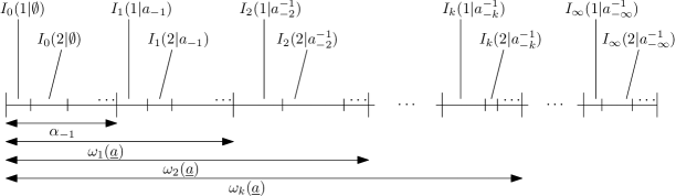
Figure 1: Illustration of the partition related to some infinite past $\underline{a}$.

With this partition in hands, the update function is simple to define:

$$F(U_{0},\underline{a}):=\sum_{a\in A}a{\bf 1}\{U_{0}\in\cup_{k\geq 0}\cup_{a\in A}I_{k}(a|a_{-k}^{-1})\}.$$

Algorithmically, this update function is practical for the following reason. If we introduce the length function

$$L(U_{0},\underline{a}):=\sum_{k\geq 0}k{\bf 1}\{U_{0}\in\cup_{a\in A}I_{k}(a|a_{-k}^{-1})\}+\infty.{\bf 1}\{U_{0}\in\cup_{a\in A}I_{\infty}(a|\underline{a})\}$$ (22)

we observe that, whenever $L(U_{0},\underline{a})\leq k<\infty$ (this occurs when $U_{0}\leq\omega_{k}(\underline{a})$) we have $F(U_{0},\underline{a})=F(U_{0},\underline{b}a_{-k}^{-1})$ for any $\underline{b}$. This means that the value of $F(U_{0},\underline{a})$ can be decided looking only at (at most) the $k$ last symbols of the infinite past $\underline{a}$. In other words, once the algorithm constructs $k$ symbols $a_{-k}^{-1}$, from, say, times $n-k$ to time $n-1$, the construction of the next symbol is possible when $L(U_{n},\underline{a})\leq k$ because this event only depends on $a_{-k}^{-1}$. This is not only a “practical” advantage, but also a mathematical advantage to prove that $\theta[0]$ (defined as (6) using this update function) is $\mathbb{P}$-a.s. finite.

Let us consider, for any $-\infty<m\leq n\leq+\infty$

$$\theta^{\prime}[m,n]:=\max\{i\leq m:\,\textrm{for any }\underline{a}\,,\,\,L(\underline{a}F_{\{i,j-1\}}(\underline{a},U_{i}^{j-1}),U_{j})\leq j-i\,,\,j=i,\ldots,n\}$$

with the convention that $\theta[m]:=\theta[m,m]$ and where $F_{\{m,n\}}(\underline{a},U_{m}^{n})$ denotes the whole constructed string based on the past $\underline{a}$, that is, for any $-\infty<m\leq n\leq+\infty$

$$F_{\{m,n\}}(\underline{a},U_{m}^{n}):=F(\underline{a},U_{m})F_{[m,m+1]}(\underline{a},U_{m}^{m+1})\ldots F_{[m,n]}(\underline{a},U_{m}^{n}).$$

Lemma 6.1

$\theta^{\prime}[0]\leq\theta[0]$.

Proof We will prove that $\theta^{\prime}[0]\in\{j\leq 0:F_{\{j,0\}}(\underline{a},U_{j}^{0})\,\,\,\textrm{does not depend on }\,\underline{a}\}.$ Assume $\theta^{\prime}[0]=-k>-\infty$. We proceed recursively. First observe that $U_{-k}\in[0,\alpha_{-1}[$ since $L(U_{-k},\underline{a})=0$ for any $\underline{a}$, and therefore, $F_{\{-k,-k\}}(\underline{a},U_{-k})=F(\underline{a},U_{-k})$ is obtained independently of $\underline{a}$. Suppose (recursion hypothesis) that for some $l\in\{1,\ldots,k-1\}$, the whole string $F_{\{-k,-l\}}(\underline{a},U_{-k}^{-l})$ has been constructed independently of $\underline{a}$. Since $L(\underline{a}F_{\{-k,-l\}}(\underline{a},U_{-k}^{-l}),U_{-l+1})\leq k-l+1$, it follows that the value of $F(\underline{a}F_{\{-k,-l\}}(\underline{a},U_{-k}^{-l}),U_{-l+1})$ can be obtained independently of $\underline{a}$, and thus, concatenating, we obtain that the whole string $F_{\{-k,-l+1\}}(\underline{a},U_{-k}^{-l+1})$ has been constructed independently of $\underline{a}$, establishing the recursion from time $-k$ to time $0$. $\square$

6.2 Definition of a block-rescaled coalescence time

Lemma 6.1 indicates that we can focus on $\theta^{\prime}[0]$ instead of $\theta[0]$. However, the direct study of $\theta^{\prime}[0]$ remains an intricate task, and our objective here is to introduce the coalescence time $\Lambda[0]$, defined by equation (26), which is easier to study. We will nevertheless need to introduce a sequence of technical definitions in order to get to its definition. Let $\{\theta^{k}\}_{k\geq-1}$ be the sequence of r.v.’s defined by $\theta^{-1}:=1$ and for any $k\geq 0$

$$\theta^{k}=\bar{\theta}[\theta^{k-1}-1],$$

and partition $-\mathbb{N}$ into disjoint blocks $\{B_{k}\}_{k\geq 0}$ where $B_{k}=\{\theta^{k},\ldots,\theta^{k-1}-1\}$.

We consider the sequence $\{\zeta_{l}\}_{l\in\mathbb{Z}}$ defined for any $i\in\mathbb{Z}$ by

$$\zeta_{l}:={\bf 1}\{U_{l}\geq\alpha_{-1}\}\sum_{k\geq 0}k.{\bf 1}\{U_{l}\in[\alpha_{k-1}^{c_{\tau}^{l-1}},\alpha_{k}^{c_{\tau}^{l-1}}[\},$$

and define for any $k\geq 0$

$$L_{k}:=\sup_{l\in B_{k}}\zeta_{l}.$$ (23)

An important advantage of this block rescalling, that we will use later, is the fact that the sequence $\{L_{k}\}_{k\geq 0}$ is i.i.d. This follows from the definition of good coalescence time, which implies that for any $j\in B_{k}$, $k\geq 0$, such that $U_{j}\geq\alpha_{-1}$, we have

$$c_{\tau}^{j-1}=\sup_{{\bf a}}|c_{\tau}(Y({\bf a})_{\theta^{k}}^{j-1})|\leq j-\theta^{k},$$ (24)

and therefore, $\zeta_{l}$ for $i\in B_{k}$ can be determined using the array $\{U_{j}\}_{j\in B_{k}}$.

Now, introduce the random variable

$$\Theta[0]=\Theta[0]({\bf U}):=\sup\{n\leq 0:L_{i}\leq i-n\,,\,\,i=n,\ldots,0\}$$ (25)

which will play the role of a coalescence time of $B_{0}$, in the block rescaled sequence. We finally define the main random variable of interest for the proof of the theorem

$$\Lambda[0]=\Lambda[0]({\bf U}):=-\sum_{i=0}^{-\Theta[0]}|B_{i}|.$$ (26)

We now state two important lemma. Lemma 6.2 ensures that $\Lambda[0]$ is indeed a coalescence time for time $0$, and Lemma 6.3 gives informations on its tail distribution.

Lemma 6.2

$\Lambda[0]\leq\theta^{\prime}[0]$.

Proof We will prove that $\Lambda[0]$ belongs to the set of coalescence times $\{i\leq 0:\,\textrm{for any }\underline{a}\,,\,\,L(\underline{a}F_{\{i,j-1\}}(\underline{a},U_{i}^{j-1}),U_{j})\leq j-i\,,\,j=i,\ldots,0\}$. We proceed in three steps.

Step 1. Observe that, for any $k\geq 0$ and any $i\in B_{k}$, $\zeta^{\prime}_{i}=i-\theta^{k}+{\bf 1}\{U_{i}\geq\alpha_{-1}\}\left(\sum_{j=1}^{L_{k}}|B_{k+j}|\right),\,\,\,\,\forall i\in B_{k}\,\textrm{ and }\,k\geq 0$, we can rewrite $\Lambda[0]$ as $\max\{i\leq m:\,\zeta^{\prime}_{j}\leq j-i\,,\,j=i,\ldots,n\}$

Step 2. Since (i) $|B_{k}|\geq 1$, $\forall k\geq 0$, (ii) for any $i\in B_{k}$ we have $L_{k}\geq\zeta_{i}$ and (iii) for any $i\in B_{k}$ such that $U_{i}\geq\alpha_{-1}$, we have

$$c_{\tau}^{i-1}=\sup_{{\bf a}}|c_{\tau}(Y({\bf a})_{\bar{\theta}[i]}^{i-1})|\leq i-\theta^{k},$$ (27)

it follows that $\zeta_{i}^{\prime}\geq\xi_{i}:={\bf 1}\{U_{i}\geq\alpha_{-1}\}c_{\tau}^{i-1}+\zeta_{i}$.

Step 3. We will prove that, for any realization ${\bf u}$ of the process ${\bf U}$ such that $\xi_{l}\leq k$, we have $L(\underline{a}F_{\{l-k,l-1\}}(\underline{a},u_{l-k}^{l-1}),u_{l})\leq k$ for any $\underline{a}\in A^{-\mathbb{N}}$. This is trivial if $u_{l}\leq\alpha_{-1}$, thus we assume that this is not the case. We have the following sequence of inequalities. First, by (13), supposing $c_{\tau}^{l-1}=m$

$$|c_{\tau}(\underline{a}F_{\{l-k,l-1\}}(\underline{a},u_{l-k}^{l-1}))|\leq c_{\tau}^{l-1}=m.$$ (28)

This implies, together with (15), that, for any $i\geq 0$,

$$\alpha_{i}^{m}=\alpha_{i}^{c_{\tau}^{l-1}}\leq\alpha_{i}^{|c_{\tau}(\underline{a}F_{\{l-k,l-1\}}(\underline{a},u_{l-k}^{l-1}))|}\leq\alpha_{i}^{c_{\tau}(\underline{a}F_{\{l-k,l-1\}}(\underline{a},u_{l-k}^{l-1}))},$$

and by (10) and (2), we have

$$\alpha_{i}^{c_{\tau}(\underline{a}F_{\{l-k,l-1\}}(\underline{a},u_{l-k}^{l-1}))}\leq\omega_{i+|c_{\tau}(\underline{a}F_{\{l-k,l-1\}}(\underline{a},u_{l-k}^{l-1}))|}(\underline{a}F_{\{l-k,l-1\}}(\underline{a},u_{l-k}^{l-1})).$$

Since $\xi_{l}\leq k$, we have, using the above inequalities

$$u_{l}\leq\alpha_{k-m}^{m}\leq\omega_{k-m+|c_{\tau}(\underline{a}F_{\{l-k,l-1\}}(\underline{a},u_{l-k}^{l-1}))|}(\underline{a}F_{\{l-k,l-1\}}(\underline{a},u_{l-k}^{l-1})).$$

According to the partition defining $F$ and $L$, this implies that the length function $L(\underline{a}F_{\{l-k,l-1\}}(\underline{a},u_{l-k}^{l-1}),u_{l})\leq k-m+|c_{\tau}(\underline{a}F_{\{l-k,l-1\}}(\underline{a},u_{l-k}^{l-1}))|$, and using one more time (28) concludes the proof of Step 3.

We complete the proof of the lemma using steps 1, 2 and 3.

$\square$

Lemma 6.3 (Key-Lemma)

Consider a kernel $P$ belonging to LC($\tau$) with good probabilistic skeleton $(\tau,p)$, and let $\bar{\theta}[0]$ be the corresponding good coalescence time.

1. If $\sum_{k\geq 1}\prod_{j=0}^{k-1}{\mathbb{P}}(L_{0}\leq i)=+\infty$, then $\Lambda[0]$ is $\mathbb{P}$-a.s. finite.

2. If $\bar{\theta}[0]$ has summable tail and $\sum_{k\geq 0}{\mathbb{P}}(L_{0}>i)<+\infty$, then $\Lambda[0]$ has summable tail.

3. If $\bar{\theta}[0]$ has exponential tail and $\{{\mathbb{P}}(L_{0}>i)\}_{k\geq 0}$ decays exponentially fast to zero, then $\Lambda[0]$ has exponential tail.

In particular, since $\Lambda[0]\leq\theta^{\prime}[0]\leq\theta[0]$, it follows that in each of these regimes, the same conclusion hold for all these coalescence times.

Proof In order to control the tail distribution of $\Lambda[0]$ (see (26)), we first need to control the tail distribution of $\Theta[0]$. Observe that $\Theta[0]$ is defined over the block rescaled sequence using the i.i.d. sequence of r.v.’s $\{L_{i}\}_{i\geq 0}$ exactly as the coalescence time of site $0$ was defined in Comets et al. (2002) (where it is denoted by $\tau[0]$). Indeed, since the $L_{i}$’s are i.i.d., and since $\mathbb{P}(L_{0}=0)\geq\mathbb{P}(|B_{0}|=1)=\alpha_{-1}>0$, we can invoke Theorem 4.1 item (iv) together with Proposition 5.1 in Comets et al. (2002) and obtain the following assertions

(6.3.1) if $\sum_{k\geq 1}\prod_{i=0}^{k-1}\mathbb{P}(L_{0}\leq i)=+\infty$, then $\Theta[0]$ is a.s. finite,

(6.3.2) if $\{\mathbb{P}(L_{0}>k)\}_{k\geq 0}$ is summable, then $\Theta[0]$ has summable tail,

(6.3.3) if $\{\mathbb{P}(L_{0}>k)\}_{k\geq 0}$ decays exponentially fast to $0$, then $\Theta[0]$ has exponential tail.

Coming back to the definition (26) of $\Lambda[0]$, we now prove items (i), (ii) and (iii) of the lemma using respectively items (6.3.1), (6.3.2) and (6.3.3) we just stated. Item (i) is direct since the sum of an a.s. finite number of random variables which are a.s. finite is a.s. finite. For item (ii),we observe that

$$\sum_{i=0}^{n-1}|B_{i}|-n\mathbb{E}|B_{0}|$$

is a martingale with respect to the filtration $\mathcal{F}((L_{0},|B_{0}|),\ldots,(L_{-i},|B_{-i}|):i\geq 0)$. Moreover, $\Theta[0]$ is a stopping time with respect to the same filtration, this follows directly from the definitions of $\Theta[0]$. Thus, by the Optional Stopping Theorem

$$\mathbb{E}\Lambda[0]=\mathbb{E}\left(\sum_{i=0}^{-\Theta[0]}|B_{i}|\right)=\mathbb{E}|B_{0}|.\mathbb{E}|\Theta[0]|,$$

which is finite by item (6.3.2) above, in the conditions of item (ii) of the key-lemma. For the proof of item (iii), we use the proof of item (iv) of Lemma 14 in Harvey et al. (2007). Let $\rho:=(2\mathbb{E}|B_{0}|)^{-1}$ and compute

$$\mathbb{P}(\Lambda[0]<-n)=\sum_{i\geq 0}\mathbb{P}(\Theta[0]=-i,\sum_{j=0}^{i}|B_{j}|>n)$$

$$\leq\sum_{i=0}^{\lfloor\rho.n\rfloor}\mathbb{P}\left(\Theta[0]=-i,\sum_{j=0}^{i}|B_{j}|>n\right)+\sum_{i\geq\lfloor\rho.n\rfloor+1}\mathbb{P}(\Theta[0]=-i)$$

$$\leq\lfloor\rho.n\rfloor\mathbb{P}\left(\left|\sum_{j=0}^{\lfloor\rho.n\rfloor}|B_{j}|-\lfloor\rho.n\rfloor\mathbb{E}|B_{0}|\right|>n/2\right)+\mathbb{P}(\Theta[0]<-\lfloor\rho.n\rfloor)$$ (29)

Because $|B_{0}|$ has exponential tail, a standard result of large deviation (see for example Corollary 27.1 in Kallenberg (2002)) shows that the first term in the last line decays exponentially in $n$. This proves item (iii) using item (6.3.3) above. $\square$

6.3 Proof of Theorem 4.1

Using Lemmas 6.1, 6.2 and 6.3, it remains to prove that $A_{m}\leq\mathbb{P}(L_{0}\leq m)$, $m\geq 0$. For any $i\geq 0$

$$\mathbb{P}(L_{0}>i)= \mathbb{P}(\sup_{j\in B_{0}}\zeta_{j}>i)=\mathbb{P}(\sum_{j=\bar{\theta}[0]}^{0}{\bf 1}\{\zeta_{j}>i\}\geq 1)\leq\mathbb{E}(\sum_{j=\bar{\theta}[0]}^{0}{\bf 1}\{\zeta_{j}>i\}).$$ (30)

We have all the ingredient for applying the Wald inequality:

• By translation invariance, we have $\mathbb{E}\zeta_{l}=\mathbb{E}\zeta_{0}$ for any $l\in\mathbb{Z}$.

• By our assumptions, $\mathbb{E}|\bar{\theta}[0]|<\infty$.

• Finally, for any $n\geq 1$,

  $$\mathbb{E}({\bf 1}\{\zeta_{-n}>i\}.{\bf 1}\{\bar{\theta}[0]\leq-n\}) =\mathbb{E}{\bf 1}\{\zeta_{-n}>i\}-\mathbb{E}({\bf 1}\{\zeta_{-n}>i\}.{\bf 1}\{\bar{\theta}[0]>-n\})$$

  $$=\mathbb{E}{\bf 1}\{\zeta_{0}>i\}-\mathbb{E}{\bf 1}\{\zeta_{-n}>i\}.\mathbb{E}({\bf 1}\{\bar{\theta}[0]>-n\})$$

  $$=\mathbb{E}{\bf 1}\{\zeta_{0}>i\}.\left[1-\mathbb{P}(\bar{\theta}[0]>-n)\right]$$

  $$=\mathbb{P}(\zeta_{0}>i).\mathbb{P}(\bar{\theta}[0]\leq-n)$$

  where, for the second line, we used the fact that $\{\bar{\theta}[0]>-n\}$ is measurable with respect to $\mathcal{F}(U_{-n+1}^{0})$, while ${\bf 1}\{\zeta_{-n}>i\}$ is $\mathcal{F}(U_{-\infty}^{-n})$-measurable.

Thanks to all these facts, we can use Wald’s equality, and obtain

$$\mathbb{P}(L_{0}>i)\leq\mathbb{E}(|\bar{\theta}[0]|+1)\mathbb{P}(\zeta_{0}>i)=\mathbb{E}(|\bar{\theta}[0]|+1)\mathbb{P}(U_{0}\geq\alpha_{i}^{c_{\tau}^{-1}}),$$

and since for any $i\geq 0$ we have $\mathbb{P}(L_{0}\leq i)\geq\mathbb{P}(L_{0}=0)\geq\alpha_{-1}$, the proof of the theorem is concluded using $A_{k}:=\left\{1-(\mathbb{E}|\bar{\theta}[0]|+1)\mathbb{P}(U_{0}>\alpha_{k}^{c_{\tau}^{-1}})\right\}\vee\alpha_{-1}$.$\hskip 71.13188pt\square$

7 Relaxing the local continuity assumption

In this section we propose an extension of the notion of local continuity. Local continuity corresponds to assume that there exists a stopping time for the reversed-time process, beyond which the decay of the dependence on the past occurs uniformly. Removing this assumption means that no stopping time can tell whether or not the past we consider is a continuity point for $P$. This idea is now formalized in the following definition.

Definition 7.1

We will say that a kernel $P$ belongs to the class of extended locally continuous with respect to some skeleton $\tau$ if for any $v\in{\vphantom{\tau}}^{<\infty}{\tau}$

$$\bar{\alpha}_{k}^{v}:=\inf_{v_{1}\in\tau}\inf_{v_{2}\in\tau}\ldots\inf_{v_{k}\in\tau}\sum_{a\in A}\inf_{\underline{z}}P(a|v\,v_{1}\,v_{2}\ldots\,v_{k}\,\underline{z})\stackrel{{\scriptstyle k\rightarrow+\infty}}{{\longrightarrow}}1.$$ (31)

We will denote this class by extLC($\tau$). The probabilistic skeleton (p.s.) of $P$ is the pair $(\tau,p)$ where $p:=\{p(a|v)\}_{a\in A,\,v\in{\vphantom{\tau}}^{<\infty}{\tau}}$,

$$p(a|v):=\inf_{\underline{z}}P(a|v\underline{z})$$ (32)

and $p(a|v)=P(a|v)$ for any $v\in{\vphantom{\tau}}^{\infty}{\tau}$.

Theorem 7.1

Assume that $P$ belongs to extLC($\tau$) with good probabilistic skeleton. Assume furthermore that the good coalescence time $\bar{\theta}[0]$ satisfies that $c_{\tau}^{j}\leq j-\bar{\theta}[0]$ for any $j\in\{\bar{\theta}[0],\ldots,0\}$. For any $k\geq 0$, denote

$$\bar{A}_{k}:=\left\{1-(\mathbb{E}|\bar{\theta}[0]|+1)\mathbb{P}(U_{0}>\bar{\alpha}_{k}^{c_{\tau}^{-1}})\right\}\vee\alpha_{-1},\,\,\,\,k\geq 0.$$

Then, we can construct for $P$, an update function $F$ and a corresponding coalescence time $\theta$ such that

1. If $\sum_{k\geq 1}\prod_{j=0}^{k-1}\bar{A}_{k}=+\infty$, then $\theta[0]$ is $\mathbb{P}$-a.s. finite.

2. If $\sum_{k\geq 0}(1-\bar{A}_{k})<+\infty$, then $\theta[0]$ has summable tail.

3. If $\bar{\theta}[0]$ has exponential tail and $\{1-\bar{A}_{k}\}_{k\geq 0}$ decays exponentially fast to zero, then $\theta[0]$ has exponential tail.

In particular, in each of these regimes, the CFTP with update function $F$ is feasible.

Observe that the assumption that $c_{\tau}^{j}\leq j-\bar{\theta}[0]$ for any $j\in\{\bar{\theta}[0],\ldots,0\}$ is a bit stronger than simply assuming that $\bar{\theta}[0]$ is good since this later assumption only implies that $c_{\tau}^{j}\leq j-\bar{\theta}[0]$ for the time indexes $j\in\{\bar{\theta}[0],\ldots,-1\}$ such that $Y_{j+1}=\star$. Nevertheless, for skeletons having terminal context $w$, $\bar{\theta}[0]:=\max\{i\leq-|w|+1:Y_{i}^{i+|w|-1}=w\}$ used in Proposition 5.1 satisfies this stronger assumption. For skeletons $\tau^{\sigma}$ as considered in Proposition 5.2, the good coalescence time $\bar{\theta}[0]:=\min\{i\geq 0:\frac{1}{i+1}\sum_{j=-i}^{0}Y({\bf 0})_{j}\geq\sigma\}$ also satisfies the stronger assumption. We now give the proof of this theorem, and then give two examples on $A=\{-1,+1\}$, and an application for creation of new skeleton that can be used for Theorem 4.1.

Proof The proof of this theorem follows exactly the same steps as the proof of Theorem 4.1. To avoid repetition, we just outline the key observation and leave the proof to the reader. Observe that, if at time $i$, the random variable $\bar{L}_{i}$ takes value $l$, this means that we have to look at a portion of the past preceding $B_{i}$ which contains $l$ concatenated contexts of $\tau$. But in the conditions of the theorem, the blocks themselves are concatenation of contexts of $\tau$, then, it is still true that we have at least $l$ concatenated contexts contained in the $l$ blocks preceding $B_{i}$.

Therefore, if $\alpha_{k}=\bar{\alpha}_{k}$, the number of blocks involved in both procedures is the same. Thus, the random variable $\bar{\Lambda}[0]$ obtained with the new decomposition has essentially the same tail distribution as $\Lambda[0]$.

Example 7.1

For any $\underline{a}\in A^{-\mathbb{N}}$, let

$$\mathcal{K}(\underline{a}):=\inf\{i\geq 1:a_{-k}=a_{-k-1},\,k\geq i\}$$

with the convention that $\mathcal{K}(\underline{a})=+\infty$ if the set is empty. Now let $P$ be defined by

$$P(1|\underline{a})=\epsilon+\frac{1}{f[\mathcal{K}(\underline{a})]},$$

where $f$ is an unbounded increasing integer valued function satisfying $f(1)\geq\frac{1}{1-2\epsilon}$. This way we get $\inf_{\underline{a}}P(-1|\underline{a})=1-\epsilon-\frac{1}{f(1)}\geq\epsilon$. We will show that this kernel has discontinuities at every point having either finitely many $-1$’s or finitely many $1$’s. Let $\mathcal{S}$ denote the set of such points and take $\underline{a}\in\mathcal{S}$. We have, for any $\underline{z}\in A^{-\mathbb{N}}\setminus\mathcal{S}$, $P(1|a_{-k}^{-1}\underline{z})=\epsilon$ for any $k$ and therefore, does not converge to $\epsilon+\frac{1}{\mathcal{K}(\underline{a})}$. On the other hand, the kernel is continuous at any $\underline{a}\in A^{-\mathbb{N}}\setminus\mathcal{S}$, since $P(1|a_{-k}^{-1}\underline{z})=\epsilon+\frac{1}{\mathcal{K}(a_{-k}^{-1}\underline{z})}$ which always converge to $\epsilon$ because $\mathcal{K}(a_{-k}^{-1}\underline{z})$ converges to $+\infty$ (or equals infinity when $\underline{z}\in A^{-\mathbb{N}}\setminus\mathcal{S}$).

The main point is that the integer $\mathcal{K}(\underline{a})$ can never be checked looking at a finite portion of the past, while both, $\mathcal{L}(\underline{a})$ and $T_{\sigma}(\underline{a})$ (used to define the kernels of Section 5.3) can be checked looking at a finite portion of the past of $\underline{a}$. This means that no matter how much we know of $\underline{a}$, we never make sure that it is indeed continuous past for $P$. We now explain why this new kernel satisfies the conditions of Theorem 7.1. First, we observe that it belongs to extLC($\tilde{\tau}$) with

$$\tilde{\tau}=\{-\underline{1}\}\cup\bigcup_{i\geq 0}\{1(-1)^{i}\}\cup\{\underline{1}\}\cup\bigcup_{i\geq 0}\{-11^{i}\}$$

since for any $k\geq 0$ and any set $\{v,v_{1},\ldots,v_{k}\}$ of elements of $\tilde{\tau}$, we have

$$\sum_{a\in A}\inf_{\underline{z}}P(a|v\,v_{1}\,v_{2}\ldots\,v_{k}\,\underline{z}) =\inf_{\underline{z}}P(1|v\,v_{1}\,v_{2}\ldots\,v_{k}\,\underline{z})+1-\sup_{\underline{z}}P(1|v\,v_{1}\,v_{2}\ldots\,v_{k}\,\underline{z})$$

$$=1-\frac{1}{f[|v|+\sum_{i=1}^{k}|v_{i}|]}$$

and therefore, $\inf_{v\in\tilde{\tau}}\bar{\alpha}^{v}_{k}=1-\frac{1}{f(2k+2)}$ which converges to $1$ as $k$ diverges. Also, observe that the p.s. $(\tilde{\tau},p)$ satisfies $p(a|v)\geq\epsilon$ for any $a\in A$ and $v\in\tilde{\tau}$, and therefore, fits the conditions of Proposition 5.1, because $\tilde{\tau}$ has $(-1)1$ and $1(-1)$ as terminal strings. It follows that $\mathbb{E}|\bar{\theta}[0]|\leq 1/\epsilon^{2}$ and thus

$$\bar{A}_{k}\geq 1-(1+\frac{1}{\epsilon^{2}})\frac{1}{f(2k+2)}.$$

According to the function $f$ we choose, we can have the three regimes of CFTP specified by Theorem 7.1.

Example 7.2

This example is taken from De Santis & Piccioni (2012) (Example 1 therein). It is defined using a sequence of real numbers $\{\theta_{n}\}_{n\geq 1}$ such that $\sum_{k\geq 1}|\theta_{k}|<1/2$, a continuous function $f:\mathbb{R}^{+}\rightarrow[0,1]$ decreasing to $0$, and the quantity

$$S_{k}(a_{-k}^{-1})=\sum_{i=1}^{k-1}{\bf 1}\{a_{-i}\neq a_{-i-1}\},$$

which counts the number of changes of signal in $a_{-k}^{-1}$. For any $\underline{a}\in A^{-\mathbb{N}}$, let

$$P(1|\underline{a})=1/2+\sum_{k\geq 1}\theta_{k}a_{-k}f(S_{k}(a_{-k}^{-1})).$$

Observe that this kernel is somewhat similar to the AR kernel (introduced in Section 5.3.1) with $\psi=\textrm{Id}$ and $\theta_{0}=1/2$, with the difference that each occurrences of signal changes in the past reduces the dependence due to the multiplicative term in the sum. The same calculation as in the case of AR processes yields

$$\omega_{k}(\underline{a})=1-2f(\beta S_{k}(a_{-k}^{-1}))\sum_{i\geq k+1}|\theta_{i}|.$$

This kernel is therefore continuous as for the AR process, with the difference that instead of a multiplicative term $\psi^{\prime}(c(a_{-k}^{-1}))$ which is bounded away from $0$ and $+\infty$ (see (20)), we now have a term $f(\beta S_{k}(a_{-k}^{-1}))$ which goes to zero for the pasts $\underline{a}$ having infinitely many changes of sign. In other words, these pasts have a faster continuity rate. Uniform continuity may not be useful because it amounts to take into account only the sequence $\{\sum_{i\geq k+1}|\theta_{i}|\}_{k\geq 0}$ which may converge too slow to zero. This kernel is also an example in which the notion of local continuity of Theorem 4.1 cannot be used, since we cannot make sure whether a given past has a finite or infinite number of sign changes looking only at a finite portion. However, it belongs to extLC($\tilde{\tau}$), since, for any $k\geq 0$ and any set $\{v,v_{1},\ldots,v_{k}\}$ of elements of $\tilde{\tau}$, denoting $l=|v|+\sum_{i=1}^{k}|v_{i}|$

$$\sum_{a\in A}\inf_{\underline{z}}P(a|v\,v_{1}\,v_{2}\ldots\,v_{k}\,\underline{z}) =\inf_{\underline{z}}P(1|v\,v_{1}\,v_{2}\ldots\,v_{k}\,\underline{z})+1-\sup_{\underline{z}}P(1|v\,v_{1}\,v_{2}\ldots\,v_{k}\,\underline{z})$$

$$=1-2f(\beta S_{l}(a_{-l}^{-1}))\sum_{i\geq l+1}|\theta_{i}|.$$

Notice that we have $S_{l}(a_{-l}^{-1}))\geq k$, since there is at least $k$ sign changes in the concatenated string $v_{k}\ldots v_{1}v$. Thus, we obtain

$$\inf_{v}\bar{\alpha}^{v}_{k}\geq 1-2f(\beta k)\sum_{i\geq 2k+3}|\theta_{i}|$$

and the same calculations as in the preceding example yields

$$\bar{A}_{k}\geq 1-(1+\frac{1}{\epsilon^{2}})2f(\beta k)\sum_{i\geq 2k+3}|\theta_{i}|.$$

Here also, according to the function $f$ we choose, we can have the three regimes of CFTP specified by Theorem 7.1. For instance, the special case of $f(x)=e^{-\beta x}$, $\beta>0,x>0$ yields an exponential tail for the coalescence time of the CFTP (regime (iii) of our theorem).

Application of Theorem 7.1

By analogy with Definition 5.2, we can define the class of kernels that satisfy the extended strong local continuity with respect to some skeleton $\tau$ (let us denote extSLC($\tau$)). These are such that for any $v\in{\vphantom{\tau}}^{<\infty}{\tau}$, there exists a positive integer $h(v)$ such that for any $k\geq h(v)$, $\bar{\alpha}_{k}^{v}=1$. The interesting point is that such kernels, when they satisfy the conditions of items (ii) or (iii) of Theorem 7.1, are good p.s.’s themselves.

In other words, we have somehow a self-feeding argument, which allows us to construct more complicated good p.s.’s from simpler ones, using Theorem 7.1. And if we can show that $P$ is a good p.s., it can be used as such in Theorem 4.1.

We now explain why the kernels $P$ belonging to extSLC($\tau$) and satisfying the assumptions of Theorem 7.1 are indeed good (see Definition 3.4). First, we observe

$$\bar{\zeta}_{l}:={\bf 1}\{U_{l}\geq\alpha_{-1}\}\sum_{k\geq 0}k.{\bf 1}\{U_{l}\in[\bar{\alpha}_{k-1}^{c_{\tau}^{l-1}},\bar{\alpha}_{k}^{c_{\tau}^{l-1}}[\}\leq{\bf 1}\{U_{l}\geq\alpha_{-1}\}h(c^{l-1}_{\tau})=:\bar{\bar{\zeta}}_{l}.$$

This inequality means that we can use $\{\bar{\bar{\zeta}}_{l}\}_{l\in\mathbb{Z}}$ to obtain another coalescent time $\bar{\bar{\Lambda}}[0]$, defined in the same way $\bar{\Lambda}[0]$ is defined using $\bar{\zeta}[0]$ (that is, just as we did in the proof of Theorem 4.1). Clearly, we will have $\bar{\bar{\Lambda}}[0]\leq\bar{\Lambda}[0]$, moreover $\bar{\bar{\Lambda}}[0]$ is a good coalescence time (see Definition 3.4) because $\bar{\bar{\zeta}}_{l}$ is $\mathcal{F}(Y_{-\infty}^{l})$-measurable. The fact that $P$ is in fact a good p.s. follows now from the fact that $\bar{\bar{\Lambda}}[0]$ has finite expectation under the assumptions of items (ii) and (iii) Theorem 7.1.

8 Concluding remarks

There are several results that follow from the existence of a CFTP scheme and the regenerative structures. Among them, bounds for the $\bar{d}$-distance, rate of decay of correlations, concentration inequalities and Functional Central Limit Theorem.

• Bounds for the $\bar{d}$-distance. Given a finite sample, it is natural to use a Markov approximation whose transition probabilities can be estimated from a sample of the infinite-order chain. A natural candidate would be the canonical $k^{\textrm{th}}$-order approximation, which is obtained by cutting off the memory after $k$ steps. Bounds on the $\bar{d}$-distance can be used to characterize the rate of convergence of estimators for stationary processes that can be approximated by $k$-steps Markov chains (see Csiszár & Talata (2010)). Gallo et al. (2011) use our perfect simulation scheme to derive new bounds for the $\bar{d}$-distance between the original chain and its canonical $k$-steps Markov approximation.

• Loss of memory and decay of correlations. CFTP allows to directly obtain explicit upper bounds for the speed of the loss of memory of the chain, as it has been showed in Comets et al. (2002). On the other hand, it is known that the decay of correlations is bounded above by this speed (see Remark 6.2.2 of Maillard (2007) for instance). Roughly speaking, this means that both, decay of correlations and speed of loss of memory are controlled by the tail distribution of the coalescence time of the CFTP.

• Concentration of measures. Another direct application of CFTP is the following result on concentration of measures, proved in Gallo & Takahashi (2011).

  Proposition 8.1

  Let ${\bf X}$ be a process that can be simulated by a CFTP algorithm with a coalescence time $\theta$. If ${\mathbb{E}}[\theta]<\infty$, then for all $\epsilon>0$ and all functions $f:A^{n}\to{\mathbb{R}}$ we have

  $${\mathbb{P}}\left(\left|f(X^{n}_{1})-{\mathbb{E}}[f(X^{n}_{1})]\right|>\epsilon\right)\leq 2\exp\left\{{-\frac{2\epsilon^{2}}{(1+{\mathbb{E}}[\theta])^{2}\|\delta f\|^{2}_{\ell_{2}({\mathbb{N}})}}}\right\}.$$

• Functional Central Limit Theorem. Under assumptions ensuring that the coalescence time of time $0$ has summable tail (basically the number of steps that have to be performed by the algorithm in order to construct the stationary chain at time $0$), the constructed chain has a regeneration scheme. Such structure has been already observed under stronger assumptions using continuity, by for example, Lalley (1986), but also more recently in Comets et al. (2002) and Gallo (2011). It is worth mentioning that using this fact, a Functional Central Limit Theorem could be derived for our chains, as it has been done by Maillard & Schöpfer (2008) under the continuity assumption. This is because, looking at their proof, we observe that it uses the regeneration property of the measure, and not the form of the conditional probabilities of the chain.

Acknowledgments

This work is part of USP Project “Mathematics, computation, language and the brain”. SG was supported by a FAPESP fellowship (grant 2009/09809-1). NG is supported by CNPq grants 475504/2008-9, 302755/2010-1 and 476764/2010-6. We thank the anonymous referees for valuable remarks that greatly improved the presentation of this work.

References

- Chazottes & Ugalde (2011) Chazottes, J. R. & Ugalde, E. (2011). On the preservation of gibbsianness under amalgamation of symbols. In: Entropy of Hidden Markov Processes and Connections to Dynamical Systems. Amsterdam: LMS Lecture Note No. 385.
- Comets et al. (2002) Comets, F., Fernandez, R. & Ferrari, P. (2002). Processes with long memory: regenerative construction and perfect simulation. Ann. Appl. Prob. 12(3), 921–943.
- Csiszár & Talata (2010) Csiszár, I. & Talata, Z. (2010). On rate of convergence of statistical estimation of stationary ergodic processes. IEEE Transactions on Information Theory 56(8), 3637–3641.
- De Santis & Piccioni (2010) De Santis, E. & Piccioni, M. (2010). A general framework for perfect simulation of long memory processes. arXiv:1004.0113v1 .
- De Santis & Piccioni (2012) De Santis, E. & Piccioni, M. (2012). Backward coalescence times for perfect simulation of chains with infinite memory. Journal in Applied Probability 49(2) , 319–337.
- den Hollander & Steif (2006) den Hollander, F. & Steif, J. E. (2006). Random walk in random scenery: a survey of some recent results. In: Dynamics & stochastics, vol. 48 of IMS Lecture Notes Monogr. Ser. Beachwood, OH: Inst. Math. Statist., pp. 53–65.
- den Hollander et al. (2005) den Hollander, F., Steif, J. E. & van der Wal, P. (2005). Bad configurations for random walk in random scenery and related subshifts. Stochastic Process. Appl. 115(7), 1209–1232. URL http://dx.doi.org/10.1016/j.spa.2005.03.001.
- Fernández et al. (2011) Fernández, R., Gallo, S. & Maillard, G. (2011). Regular -measures are not always gibbsian. Electron. J. Prob. 16(3), 732–740.
- Foss & Konstantopoulos (2003) Foss, S. & Konstantopoulos, T. (2003). Extended renovation theory and limit theorems for stochastic ordered graphs. Markov Process. Related Fields 9(3), 413–468.
- Gallo (2011) Gallo, S. (2011). Chains with unbounded variable length memory: perfect simulation and a visible regeneration scheme. Adv. in Appl. Probab. 43(3), 735–759.
- Gallo & Garcia (2010) Gallo, S. & Garcia, N. L. (2010). Perfect simulation for stochastic chains of infinite memory: relaxing the continuity assumption. ArXiv:1005.5459 .
- Gallo et al. (2011) Gallo, S., Lerasle, M. & Yasumasa Takahashi, D. (2011). Upper Bounds for Markov Approximations of Ergodic Processes. ArXiv:1107.4353 .
- Gallo & Takahashi (2011) Gallo, S. & Takahashi, D. Y. (2011). Attractive regular stochastic chains: perfect simulation and phase transition. ArXiv e-prints .
- Garivier (2011) Garivier, A. (2011). A Propp-Wilson perfect simulation scheme for processes with long memory. ArXiv: 1106.5971 .
- Harvey et al. (2007) Harvey, N., Holroyd, A. E., Peres, Y. & Romik, D. (2007). Universal finitary codes with exponential tails. Proc. Lond. Math. Soc. (3) 94(2), 475–496. URL http://dx.doi.org/10.1112/plms/pdl018.
- Kalikow (1990) Kalikow, S. (1990). Random Markov processes and uniform martingales. Israel J. Math. 71(1), 33–54. URL http://dx.doi.org/10.1007/BF02807249.
- Kallenberg (2002) Kallenberg, O. (2002). Foundations of modern probability. Probability and its Applications (New York). New York: Springer-Verlag, second ed.
- Lalley (1986) Lalley, S. P. (1986). Regenerative representation for one-dimensional Gibbs states. Ann. Probab. 14(4), 1262–1271.
- Maes et al. (2000) Maes, C., Redig, F., Takens, F., van Moffaert, A. & Verbitski, E. (2000). Intermittency and weak Gibbs states. Nonlinearity 13(5), 1681–1698. URL http://dx.doi.org/10.1088/0951-7715/13/5/314.
- Maes et al. (1999) Maes, C., Redig, F., Van Moffaert, A. & Leuven, K. U. (1999). Almost Gibbsian versus weakly Gibbsian measures. Stochastic Process. Appl. 79(1), 1–15. URL http://dx.doi.org/10.1016/S0304-4149(98)00083-0.
- Maillard (2007) Maillard, G. (2007). Introduction to chains with complete connections. Lecture notes at Écoles Polytechnique Fédérale de Lausanne URL http://www.latp.univ-mrs.fr/$∼$maillard/Greg/Publications$_$files/main.pdf.
- Maillard & Schöpfer (2008) Maillard, G. & Schöpfer, S. (2008). A functional central limit theorem for regenerative chains. Markov Process. Related Fields 14(4), 583–598.
- Propp & Wilson (1996) Propp, J. G. & Wilson, D. B. (1996). Exact sampling with coupled Markov chains and applications to statistical mechanics. In: Proceedings of the Seventh International Conference on Random Structures and Algorithms (Atlanta, GA, 1995), vol. 9.
- Rissanen (1983) Rissanen, J. (1983). A universal data compression system. IEEE Trans. Inform. Theory 29(5), 656–664.
- van Enter et al. (2008) van Enter, A. C. D., Redig, F. & Verbitskiy, E. (2008). Gibbsian and non-Gibbsian states at Eurandom. Statist. Neerlandica 62(3), 331–344. URL http://dx.doi.org/10.1111/j.1467-9574.2008.00394.x.