GLOBAL SEARCH BASED ON EFFICIENT DIAGONAL PARTITIONS AND A SET OF LIPSCHITZ CONSTANTS

Abstract

In the paper, the global optimization problem of a multidimensional “black-box” function satisfying the Lipschitz condition over a hyperinterval with an unknown Lipschitz constant is considered. A new efficient algorithm for solving this problem is presented. At each iteration of the method a number of possible Lipschitz constants is chosen from a set of values varying from zero to infinity. This idea is unified with an efficient diagonal partition strategy. A novel technique balancing usage of local and global information during partitioning is proposed. A new procedure for finding lower bounds of the objective function over hyperintervals is also considered. It is demonstrated by extensive numerical experiments performed on more than 1600 multidimensional test functions that the new algorithm shows a very promising performance.

1 Introduction

Many decision-making problems arising in various fields of human activity (technological processes, economic models, etc.) can be stated as global optimization problems (see, e.g., [7, 26, 33]). Objective functions describing real-life applications are very often multiextremal, non-differentiable, and hard to be evaluated. Numerical techniques for finding solutions to such problems have been widely discussed in literature (see, e.g., [5, 14, 15, 26, 33]).

In this paper, the Lipschitz global optimization problem is considered. This type of optimization problems is sufficiently general both from theoretical and applied points of view. In fact, it is based on a rather natural assumption that any limited change in the parameters of the objective function yields some limited changes in the characteristics of the object’s performance. The knowledge of a bound on the rate of change of the objective function, expressed by the Lipschitz constant, allows one to construct global optimization algorithms and to prove their convergence (see, e.g., [14, 15, 26, 33]).

Mathematically, the global optimization problem considered in the paper can be formulated as minimization of a multidimensional multiextremal “black-box” function that satisfies the Lipschitz condition over a domain $D\subset\mathbb{R}^{N}$ with an unknown constant $L$, i.e., finding the value $f^{*}$ and points $x^{*}$ such that

$$f^{*}=f(x^{*})=\min_{x\in D}f(x),$$ (1)

$$|f(x^{\prime})-f(x^{\prime\prime})|\leq L\|x^{\prime}-x^{\prime\prime}\|,\hskip 8.53581ptx^{\prime},x^{\prime\prime}\in D,\hskip 11.38109pt0<L<\infty,$$ (2)

where

$$D=[a,b\,]=\{x\in\mathbb{R}^{N}:a(j)\leq x(j)\leq b(j),\,1\leq j\leq N\},$$ (3)

$a$, $b$ are given vectors in $\mathbb{R}^{N}$, and $\|\cdot\|$ denotes the Euclidean norm.

The function $f(x)$ is supposed to be non-differentiable. Hence, optimization methods using derivatives cannot be used for solving problem (1)–(3). It is also assumed that evaluation of the objective function at a point (also referred to as a ‘function trial’) is a time-consuming operation.

Numerous algorithms have been proposed (see, e.g., [5, 14, 15, 18, 21, 23, 26, 27, 29, 32, 33]) for solving problem (1)–(3). One of the main questions to be considered in this occasion is: How can the Lipschitz constant $L$ be specified? There are several approaches to specify the Lipschitz constant. First of all, it can be given a priory (see, e.g., [14, 15, 23, 27, 32]). This case is very important from the theoretical viewpoint but is not frequently encountered in practice. The more promising and practical approaches are based on an adaptive estimation of $L$ in the course of the search. In such a way, algorithms can use either a global estimate of the Lipschitz constant (see, e.g., [21, 26, 33]) valid for the whole region $D$ from (3), or local estimates $L_{i}$ valid only for some subregions $D_{i}\subseteq D$ (see, e.g., [20, 24, 29, 30, 33]).

Since the Lipschitz constant has a significant influence on the convergence speed of the Lipschitz global optimization algorithms, the problem of its specifying is of the great importance. In fact, accepting too high value of $L$ for a concrete objective function means assuming that the function has complicated structure with sharp peaks and narrow attraction regions of minimizers within the whole admissible region. Thus, too high value of $L$ (if it does not correspond to the real behavior of the objective function) leads to a slow convergence of the algorithm to the global minimizer.

Global optimization algorithms using in their work a global estimate of $L$ (or some value of $L$ given a priori) do not take into account local information about behavior of the objective function over every small subregion of $D$. As it has been demonstrated in [29, 30, 33], estimating local Lipschitz constants allows us to accelerate significantly the global search. Naturally, balancing between local and global information must be performed in an appropriate way to avoid the missing of the global solution.

Recently, an interesting approach unifying usage of local and global information during the global search has been proposed in [18]. At each iteration of this new algorithm, called DIRECT, instead of only one estimate of the Lipschitz constant a set of possible values of $L$ is used.

As many Lipschitz global optimization algorithms, DIRECT tries to find the global minimizer by partitioning the search hyperinterval $D$ into smaller hyperintervals $D_{i}$ using a particular partition scheme described in [18]. The objective function is evaluated only at the central point of a hyperinterval. Each hyperinterval $D_{i}$ of a current partition of $D$ is characterized by a lower bound of the objective function over this hyperinterval. It is calculated similarly to [27, 32] taking into account the Lipschitz condition (2). A hyperinterval $D_{i}$ is selected for a further partitioning if and only if for some value $\tilde{L}>0$ (which estimates the unknown constant $L$) it has the smallest lower bound of $f(x)$ with respect to the other hyperintervals. By changing $\tilde{L}$ from zero to infinity, at each iteration DIRECT selects several ‘potentially optimal’ hyperintervals (see [10, 13, 18]) in such a way that for a particular estimate of the Lipschitz constant the objective function could have the smallest lower bound over every potentially optimal hyperinterval.

Due to its simplicity and efficiency, DIRECT has been widely adopted in practical applications (see, e.g., [1, 2, 3, 4, 10, 13, 22, 35]). In fact, DIRECT is a derivative-free deterministic algorithm which does not require multiply runs. It has only one parameter which is easy to set (see [18]). The center-sampling partition strategy of DIRECT reduces the computational complexity in high-dimensional spaces allowing DIRECT to demonstrate good performance results (see [11, 18]).

However, some aspects which can limit the applications of DIRECT have been pointed out by several authors (see, e.g., [4, 6, 13, 17]). First of all, it is difficult to apply for DIRECT some meaningful stopping criterion, such as, for example, stopping on achieving a desired accuracy in solution. This happens because DIRECT does not use a single estimate of the Lipschitz constant but a set of possible values of $L$. Although several attempts of introducing a reasonable criterion of arrest have been done (see, e.g., [2, 4, 10, 13]), termination of the search process caused by exhaustion of the available computing resources (such as maximal number of function trials) remains the most interesting for practical engineering applications.

Another important observation regarding DIRECT is related to the partition and sampling strategies adopted by the algorithm (see [18]) which simplicity turns into some problems. As it has been outlined in [4, 6, 22], DIRECT is quick to locate regions of local optima but slow to converge to the global one. This can happen for several reasons. The first one is a redundant (especially in high dimensions, see [17]) partition of hyperintervals along all longest sides. The next cause of DIRECT’s slow convergence can be excessive partition of many small hyperintervals located in the vicinity of local minimizers which are not global ones. Finally, DIRECT — like all center-sampling partitioning schemes — uses a relatively poor information about behavior of the objective function $f(x)$. This information is obtained by evaluating $f(x)$ only at one central point of each hyperinterval without considering the adjacent hyperintervals. Due to this fact, DIRECT can manifest slow convergence (as it has been highlighted in [16]) in cases when the global minimizer lies at the boundary of the admissible region $D$ from (3).

There are several modifications to the original DIRECT algorithm. For example, in [17], partitioning along only one long side is suggested to accelerate convergence in high dimensions. The problem of stagnation of DIRECT near local minimizers (emphasized, e.g., in [6]) can be attacked by changing the parameter of the algorithm (see [18]) preventing DIRECT from being too local in its orientation (see [6, 10, 13, 17, 18]). But in this case the algorithm becomes too sensitive to tuning such a parameter, especially for difficult “black-box” global optimization problems (1)–(3). In [1, 35], another modification to DIRECT, called ‘aggressive DIRECT’, has been proposed. It subdivides all hyperintervals with the smallest function value for each hyperinterval size. This results in more hyperintervals partitioned at every iteration, but the number of hyperintervals to be subdivided grows up significantly. In [10, 11], the opposite idea which is more biased toward local improvement of the objective function has been studied. Results obtained in [10, 11] demonstrate that this modification seems to be more suitable for low dimensional problems with a single global minimizer and a few local minimizers.

The goal of this paper is to present a new algorithm which would be oriented (in contrast with the algorithm from [10, 11]) on solving ‘difficult’ multidimensional multiextremal “black-box” problems (1)–(3). It uses a new technique for selection of hyperintervals to be subdivided which is unified with a new diagonal partition strategy. A new procedure for estimation of lower bounds of the objective function over hyperintervals is combined with the idea (introduced in DIRECT) of usage of a set of Lipschitz constants instead of a unique estimate. As demonstrated by extensive numerical results, application of the new algorithm to minimizing hard multidimensional “black-box” functions leads to significant improvements.

The paper is organized as follows. In Section 2, a theoretical background of the new algorithm — a new partition strategy, a new technique for lower bounding of the objective function over hyperintervals, and a procedure for selection of ‘non-dominated’ hyperintervals for eventual partitioning — is presented. Section 3 is dedicated to description of the algorithm and to its convergence analysis. Finally, Section 4 contains results of numerical experiments executed on more than 1600 test functions.

2 Theoretical background

This section consists of the following three parts. First, a new partition strategy developed in the framework of diagonal approach is described. The second part presents a new procedure for estimation of lower bounds of the objective function over hyperintervals. The third part is dedicated to description of a procedure for determining non-dominated hyperintervals — hyperintervals that have the smallest lower bound for some particular estimate of the Lipschitz constant.

2.1 Partition strategy

In global optimization algorithms, various techniques for adaptive partition of the admissible region $D$ into a set of hyperintervals $D_{i}$ are used (see, e.g., [14, 18, 26, 31]) for solving (1)–(3). A current partition $\{D^{k}\}$ of $D$ in the course of an iteration $k\geq 1$ of an algorithm can be represented as

$$D=\cup_{i=1}^{m(k)+\Delta m(k)}D_{i},\ D_{i}\cap D_{j}=\delta(D_{i})\cap\delta(D_{j}),\ i\neq j.$$ (4)

Here, $\delta(D_{i})$ denotes the boundary of $D_{i}$, $m(k)$ is the number of hyperintervals at the beginning of the iteration $k$, and $\Delta m(k)$ is the current number of new hyperintervals produced during the $k$-th iteration. For example, if only one new hyperinterval is generated at every iteration then $\Delta m(k)=1$.

Over each hyperinterval $D_{i}\in\{D^{k}\}$, approximation of $f(x)$ is based on results obtained by evaluating $f(x)$ at some points $x\in D$. For example, DIRECT [18] involves partitioning with evaluation of $f(x)$ at the central points of hyperintervals (note that for DIRECT the number $\Delta m(k)$ in (4) can be greater than 1).

In this paper, the diagonal approach proposed in [25, 26] is considered. In this approach, the function $f(x)$ is evaluated only at two vertices $a_{i}$ and $b_{i}$ of the main diagonals of each hyperinterval $D_{i}$ independently of the problem dimension (recall that each evaluation of $f(x)$ is a time-consuming operation).

Among attractions of the diagonal approach there are the following two. First, the objective function is evaluated at two points at each hyperinterval. Thus, diagonal algorithms obtain a more complete information about the objective function than central-sampling methods. Second, many efficient one-dimensional global optimization algorithms can be easily extended to the multivariate case by means of the diagonal scheme (see, e.g, [20, 21, 24, 25, 26]).

As shown in [21, 31], diagonal global optimization algorithms based on widely used partition strategies (such as bisection or partition $2^{N}$ used in [25, 26]) produce many redundant trials of the objective function. This redundancy slows down the algorithm execution because of high time required for the evaluations of $f(x)$. It also increases the computer memory allocated for storing the redundant information.

The new partition strategy proposed in [31] (see also [21]) overcomes these drawbacks of conventional diagonal partition strategies. We start its description by a two-dimensional example in Fig. 1. In this figure, partitions of the admissible region $D$ produced by the algorithm at the initial iterations are presented. We suppose just for simplicity that at each iteration only one hyperinterval can be subdivided. Trial points of $f(x)$ are represented by black dots. The numbers around these dots indicate iterations at which the objective function is evaluated at the corresponding points. The terms ‘interval’ and ‘subinterval’ will be used to denote two-dimensional rectangular domains.

In Fig. 1a, situation after the first two iterations is presented. At the first iteration, the objective function $f(x)$ is evaluated at the vertices $a$ and $b$ of the search domain $D=[a,b]$. At the next iteration, the interval $D$ is subdivided into three subintervals of equal area (equal volume in general case). This subdivision is performed by two lines (hyperplanes) orthogonal to the longest edge of $D$ and passing through points $u$ and $v$ (see Fig. 1a). The objective function is evaluated at both points $u$ and $v$.

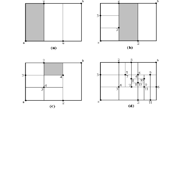
Fig. 1: An example of subdivisions by a new partition strategy.

Suppose that the interval shown in grey in Fig. 1a is chosen for the further partitioning. Thus, at the third iteration, three smaller subintervals appear (see Fig. 1b). It seems that a trial point of the third iteration is redundant for the interval (shown in grey in Fig. 1b) selected for the next splitting. But in reality, Fig. 1c demonstrates that one of the two points of the fourth iteration coincides with the point 3 at which $f(x)$ has already been evaluated. Therefore, there is no need to evaluate $f(x)$ at this point again, since the function value obtained at the previous iteration can be used. This value can be stored in a special vertex database and is simply retrieved when it is necessary without reevaluation of the function. For example, Fig. 1d illustrates situation after 11 iterations. Among 22 points at which the objective function is to be evaluated, there are 5 repeated points. That is, $f(x)$ is evaluated 17 rather than 22 times. Note also that the number of generated intervals (equal to 21) is greater than the number of trial points (equal to 17). Such a difference becomes more pronounced in the course of further subdivisions (see [21]).

Let us now describe the general procedure of hyperinterval subdivision. Without loss of generality, hereafter we assume that the admissible region $D$ in (3) is an $N$-dimensional hypercube. Suppose that at the beginning of an iteration $k\geq 1$ of the algorithm the current partition $\{D^{k}\}$ of $D=[a,b]$ consists of $m(k)$ hyperintervals and $\Delta m(k)\geq 0$ new hyperintervals have been already obtained. Let a hyperinterval $D_{t}=[a_{t},b_{t}]$ be chosen for partitioning too. The operation of partitioning the selected hyperinterval $D_{t}$ is performed as follows (we omit the iteration index in the formulae).

Step 1.

Determine points $u$ and $v$ by the following formulae

$$u=(a(1),\ldots,a(i-1),a(i)+\frac{2}{3}(b(i)-a(i)),a(i+1),\ldots,a(N)),$$ (5)

$$v=(b(1),\ldots,b({i-1}),b(i)+\frac{2}{3}(a(i)-b(i)),b(i+1),\ldots,b(N)),$$ (6)

where $a(j)=a_{t}(j),\ b(j)=b_{t}(j),\ 1\leq j\leq N$, and $i$ is given by the equation

$$i=\arg\min\,\max_{1\leq j\leq N}|b(j)-a(j)|.$$ (7)

Get (evaluate or read from the vertex database) the values of the objective function $f(x)$ at the points $u$ and $v$.

Step 2.

Divide the hyperinterval $D_{t}$ into three hyperintervals of equal volume by two parallel hyperplanes that are perpendicular to the longest edge $i$ of $D_{t}$ and pass through the points $u$ and $v$.

The hyperintervals $D_{t}$ is so substituted by three new hyperintervals with indices $t^{\prime}=t$, $m+\Delta m+1$, and $m+\Delta m+2$ determined by the vertices of their main diagonals

$$a_{t^{\prime}}=a_{m+\Delta m+2}=u,\ b_{t^{\prime}}=b_{m+\Delta m+1}=v,$$ (8)

$$a_{m+\Delta m+1}=a_{t},\ b_{m+\Delta m+1}=v,$$ (9)

$$a_{m+\Delta m+2}=u,\ b_{m+\Delta m+2}=b_{t}.$$ (10)

Step 3.

Augment the number of hyperintervals generated during the iteration $k$:

$$\Delta m=\Delta m(k):=\Delta m(k)+2.$$ (11)

The existence of a special indexing of hyperintervals establishing links between hyperintervals generated at different iterations has been theoretically demonstrated in [31]. It allows one to store information about vertices and the corresponding values of $f(x)$ in a special database avoiding in such a manner redundant evaluations of $f(x)$. The objective function value at a vertex is calculated only once, stored in the database, and read when required. The new partition strategy generates trial points in such a way that one vertex where $f(x)$ is evaluated can belong to several (up to $2^{N}$) hyperintervals (see, for example, a trial point at the 8-th iteration in Fig. 1d). Since the time-consuming operation of evaluation of the function is replaced by a significantly faster operation of reading (up to $2^{N}$ times) the function values from the database, the new partition strategy considerably speeds up the search and also leads to saving computer memory. It is particularly important that the advantage of the new scheme increases with the growth of the problem dimension (see [21, 31]).

The new strategy can be viewed also as a procedure generating a new type of space-filling curve — adaptive diagonal curve. This curve is constructed on the main diagonals of hyperintervals obtained during subdivision of $D$. The objective function is approximated over the multidimensional region $D$ by evaluating $f(x)$ at the points of one-dimensional adaptive diagonal curve. The order of partition of this curve is different within different subintervals of $D$. If selection of hyperintervals for partitioning is realized appropriately in an algorithm, the curve condenses in the vicinity of the global minimizers of $f(x)$ (see [21, 31]).

2.2 Lower bounds

Let us suppose that at some iteration $k>1$ of the global optimization algorithm the admissible region $D$ has been partitioned into hyperintervals $D_{i}\in\{D^{k}\}$ defined by their main diagonals $[a_{i},b_{i}]$. At least one of these hyperintervals should be selected for further partitioning. In order to make this selection, the algorithm estimates the goodness (or, in other words, characteristics) of the generated hyperintervals with respect to the global search. The best (in some predefined sense) characteristic obtained over some hyperinterval $D_{t}$ corresponds to a higher possibility to find the global minimizer within $D_{t}$. This hyperinterval is subdivided at the next iteration of the algorithm. Naturally, more than one ‘promising’ hyperinterval can be partitioned at every iteration.

One of the possible characteristics of a hyperinterval can be an estimate of the lower bound of $f(x)$ over this hyperinterval. Once all lower bounds for all hyperintervals of the current partition $\{D^{k}\}$ have been calculated, the hyperinterval with the smallest lower bound can be selected for the further partitioning.

Different approaches to finding lower bounds of $f(x)$ have been proposed in literature (see, e.g., [14, 18, 23, 26, 27, 32, 33]) for solving problem (1)–(3). For example, given the Lipschitz constant $L$, in [14, 23, 27] a support function for $f(x)$ is constructed as the upper envelope of a set of $N$-dimensional circular cones of the slope $L$. Trial points of $f(x)$ are coordinates of the vertices of the cones. At each iteration, the global minimizer of the support function is determined and chosen as a new trial point. Finding such a point requires analyzing the intersections of all cones and, generally, is a difficult and time-consuming task, especially in high dimensions.

If a partition of $D$ into hyperintervals is used, each cone can be considered over the corresponding hyperinterval, independently from the other cones. This allows one (see, e.g., [14, 18, 20, 26]) to avoid the necessity of establishing the intersections of the cones and to simplify the lower bound estimation. For example, multidimensional DIRECT algorithm [18] uses one cone with symmetry axis passed through a central point of a hyperinterval for lower bounding $f(x)$ over this hyperinterval. The lower bound is obtained on the boundary of the hyperinterval. This approach is simple, but it gives a too rough estimate of the minimum function value over the hyperinterval.

The more accurate estimate is achieved when two trial points over a hyperinterval are used for constructing a support function for $f(x)$. These points can be, for example, the vertices $a_{i}$ and $b_{i}$ of the main diagonal of a hyperinterval $D_{i}\in\{D^{k}\}$ (see, e.g., [20, 21, 25, 26, 31]). In this case, the objective function (due to the Lipschitz condition (2)) must lie above the intersection of the $N$-dimensional cones $C_{1}(x,L)$ and $C_{2}(x,L)$ (see the two-dimensional example in Fig. 2a). These cones have the slope $L$ and are limited by the boundaries of the hyperinterval $D_{i}$. The vertices of the cones (in $(N+1)$-dimensional space) are defined by the coordinates $(a_{i},f(a_{i}))$ and $(b_{i},f(b_{i}))$, respectively. In such a way, the lower bound of $f(x)$ is more precise with respect to the central-sampling strategy. Algorithms using this approach are called diagonal (see, e.g., [20, 21, 25, 26, 31]).

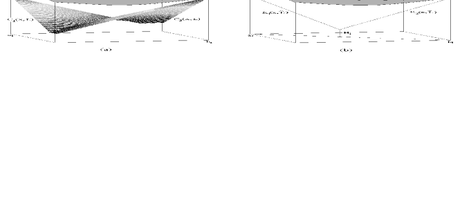
Fig. 2: Estimation of the lower bound of $f(x)$ over an interval $D_{i}=[a_{i},b_{i}]$.

In the new diagonal algorithm proposed in this paper, the objective function is also evaluated at two points of a hyperinterval $D_{i}=[a_{i},b_{i}]$. Instead of constructing a support function for $f(x)$ over the whole hyperinterval $D_{i}$, we use a support function for $f(x)$ only over the one-dimensional segment $[a_{i},b_{i}]$. This support function is the maximum of two linear functions $K_{1}(x,\hat{L})$ and $K_{2}(x,\hat{L})$ passing with the slopes $\pm\hat{L}$ through the vertices $a_{i}$ and $b_{i}$ (see Fig. 2b). The lower bound of $f(x)$ over the diagonal $[a_{i},b_{i}]$ of $D_{i}$ is calculated similarly to [27, 32] at the intersection of the lines $K_{1}(x,\hat{L})$ and $K_{2}(x,\hat{L})$ and is given by the following formula (see [20, 25, 26])

$$R_{i}=R_{i}(\hat{L})=\frac{1}{2}(f(a_{i})+f(b_{i})-\hat{L}\|b_{i}-a_{i}\|),\hskip 14.22636pt0<L\leq\hat{L}<\infty.$$ (12)

A valid estimate of the lower bound of $f(x)$ over $D_{i}$ can be obtained from (12) if an overestimate $\hat{L}$ of the Lipschitz constant $L$ is used. As it has been proved in [25, 26], inequality

$$\hat{L}\geq 2L$$ (13)

guarantees that the value $R_{i}$ from (12) is the lower bound of $f(x)$ over the whole hyperinterval $D_{i}$. Thus, the lower bound of the objective function over the whole hyperinterval $D_{i}\subseteq D$ can be estimated considering $f(x)$ only along the main diagonal $[a_{i},b_{i}]$ of $D_{i}$.

A more precise than (13) condition ensuring that

$$R_{i}(\hat{L})\leq f(x),\hskip 14.22636ptx\in D_{i},$$

is proved in the following theorem.

Theorem 2.1.

Let $L$ be the known Lipschitz constant for $f(x)$ from (2), $D_{i}=[a_{i},b_{i}]$ be a hyperinterval of a current partition $\{D^{k}\}$, and $f^{*}_{i}$ be the minimum function value over $D_{i}$, i.e.,

$$f^{*}_{i}=f(x^{*}_{i}),\hskip 14.22636ptx^{*}_{i}=\arg\min_{x\in D_{i}}f(x).$$ (14)

If an overestimate $\hat{L}$ in (12) satisfies inequality

$$\hat{L}\geq\sqrt{2}L,$$ (15)

then $R_{i}(\hat{L})$ from (12) is the lower bound of $f(x)$ over $D_{i}$, i.e., $R_{i}(\hat{L})\leq f^{*}_{i}$.

Proof. Since $x^{*}_{i}$ from (14) belongs to $D_{i}$ and $f(x)$ satisfies the Lipschitz condition (2) over $D_{i}$, then the following inequalities hold

$$f(a_{i})-f^{*}_{i}\leq L\|a_{i}-x^{*}_{i}\|,$$

$$f(b_{i})-f^{*}_{i}\leq L\|b_{i}-x^{*}_{i}\|.$$

By summarizing these inequalities and using the following result from [24, Lemma 2]

$$\max_{x\in D_{i}}(\|a_{i}-x\|+\|b_{i}-x\|)\leq\sqrt{2}\|b_{i}-a_{i}\|,$$

we obtain

$$f(a_{i})+f(b_{i})\leq 2f^{*}_{i}+L(\|a_{i}-x^{*}_{i}\|+\|b_{i}-x^{*}_{i}\|)\leq$$

$$\leq 2f^{*}_{i}+L\max_{x\in D_{i}}(\|a_{i}-x\|+\|b_{i}-x\|)\leq 2f^{*}_{i}+\sqrt{2}L\|b_{i}-a_{i}\|.$$

Then, from the last inequality and (15) we can deduce that the following estimate holds for the value $R_{i}$ from (12)

$$R_{i}(\hat{L})\leq\frac{1}{2}(2f^{*}_{i}+\sqrt{2}L\|b_{i}-a_{i}\|-\hat{L}\|b_{i}-a_{i}\|)=$$

$$=f^{*}_{i}+\frac{1}{2}\underbrace{(\sqrt{2}L-\hat{L})}_{\leq 0}\|b_{i}-a_{i}\|\leq f^{*}_{i}.\qquad\end@proof$$

Theorem 2.1 allows us to obtain a more precise lower bound $R_{i}$ with respect to [25, 26] where estimate (13) is considered.

2.3 Finding non-dominated hyperintervals

Let us now consider a diagonal partition $\{D^{k}\}$ of the admissible region $D$, generated by the new subdivision strategy from Section 2.1. Let a positive value $\tilde{L}$ be chosen as an estimate of the Lipschitz constant $L$ from (2) and lower bounds $R_{i}(\tilde{L})$ of the objective function over hyperintervals $D_{i}\in\{D^{k}\}$ be calculated by formula (12). Using the obtained lower bounds of $f(x)$, the relation of domination can be established between every two hyperintervals of a current partition $\{D^{k}\}$ of $D$.

Definition 2.1.

Given an estimate $\tilde{L}>0$ of the Lipschitz constant $L$ from (2), a hyperinterval $D_{i}\in\{D^{k}\}$ dominates a hyperinterval $D_{j}\in\{D^{k}\}$ with respect to $\tilde{L}$ if

$$R_{i}(\tilde{L})<R_{j}(\tilde{L}).$$

A hyperinterval $D_{t}\in\{D^{k}\}$ is said non-dominated with respect to $\tilde{L}>0$ if for the chosen value $\tilde{L}$ there is no other hyperinterval in $\{D^{k}\}$ which dominates $D_{t}$.

Each hyperinterval $D_{i}=[a_{i},b_{i}]\in\{D^{k}\}$ can be represented by a dot in a two-dimensional diagram (see Fig. 3) similar to that used in DIRECT for representing hyperintervals with $f(x)$ evaluated only at one point. The horizontal coordinate $d_{i}$ and the vertical coordinate $F_{i}$ of the dot are defined as follows

$$d_{i}=\frac{\|b_{i}-a_{i}\|}{2},\hskip 8.53581ptF_{i}=\frac{f(a_{i})+f(b_{i})}{2},\hskip 8.53581pta_{i}\neq b_{i}.$$ (16)

Note that a point ($d_{i},F_{i}$) in the diagram can correspond to several hyperintervals with the same length of the main diagonals and the same sum of the function values at their vertices.

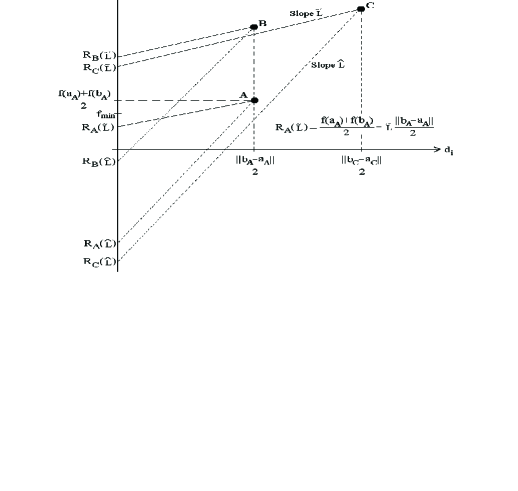
Fig. 3: Graphical interpretation of lower bounds of $f(x)$ over hyperintervals.

For the sake of illustration, let us consider a hyperinterval $D_{A}$ with the main diagonal $[a_{A},b_{A}]$. This hyperinterval is represented by the dot $A$ in Fig. 3. Assuming an estimate of the Lipschitz constant equal to $\tilde{L}$ (such that condition (15) is satisfied), a lower bound of $f(x)$ over the hyperinterval $D_{A}$ is given by the value $R_{A}(\tilde{L})$ from (12). This value is the vertical coordinate of the intersection point of the line passed through the point $A$ with the slope $\tilde{L}$ and the vertical coordinate axis (see Fig. 3). In fact, as it can be seen from (12), intersection of the line with the slope $\tilde{L}$ passed through any dot representing a hyperinterval in the diagram of Fig. 3 and the vertical coordinate axis gives us the lower bound (12) of $f(x)$ over the corresponding hyperinterval.

Note that the points on the vertical axis ($d_{i}=0$) do not represent any hyperinterval. The axis is used to express such values as lower bounds, the current minimum value of the function, etc. It should be highlighted that the current best value $f_{min}$ is always smaller than or equal to the vertical coordinate of the lowest dot (dot $A$ in Fig. 3). Note also that the vertex at which this value has been obtained can belong to a hyperinterval, different from that represented by the lowest dot in the diagram.

By using this graphical representation, it is easy to determine whether a hyperinterval dominates (with respect to a given estimate of the Lipschitz constant) some other hyperinterval from a partition $\{D^{k}\}$. For example, for the estimate $\tilde{L}$ the following inequalities are satisfied (see Fig. 3)

$$R_{A}(\tilde{L})<R_{C}(\tilde{L})<R_{B}(\tilde{L}).$$

Therefore, with respect to $\tilde{L}$ the hyperinterval $D_{A}$ (dot $A$ in Fig. 3) dominates both hyperintervals $D_{B}$ (dot $B$) and $D_{C}$ (dot $C$), while $D_{C}$ dominates $D_{B}$. If our partition $\{D^{k}\}$ consists only of these three hyperintervals, the hyperinterval $D_{A}$ is non-dominated with respect to $\tilde{L}$.

If a higher estimate $\hat{L}>\tilde{L}$ of the Lipschitz constant is considered (see Fig. 3), the hyperinterval $D_{A}$ still dominates the hyperinterval $D_{B}$ with respect to $\hat{L}$, since $R_{A}(\hat{L})<R_{B}(\hat{L})$. But $D_{A}$ in its turn is dominated by the hyperinterval $D_{C}$ with respect to $\hat{L}$, because $R_{A}(\hat{L})>R_{C}(\hat{L})$ (see Fig. 3). Thus, for the chosen estimate $\hat{L}$ the unique non-dominated hyperinterval with respect to $\hat{L}$ is $D_{C}$, and not $D_{A}$ as previously.

As we can see from this simple example, some hyperintervals (as the hyperinterval $D_{B}$ in Fig. 3) are always dominated by another hyperintervals, independently on the chosen estimate of the Lipschitz constant $L$. The following result formalizing this fact takes place.

Lemma 2.1.

Given a partition $\{D^{k}\}$ of $D$ and the subset $\{D^{k}\}_{d}$ of hyperintervals having the main diagonals equal to $d>0$, for any estimate $\tilde{L}>0$ of the Lipschitz constant a hyperinterval $D_{t}\in\{D^{k}\}_{d}$ dominates a hyperinterval $D_{j}\in\{D^{k}\}_{d}$ if and only if

$$F_{t}=\min\{F_{i}:\hskip 5.69054ptD_{i}\in\{D^{k}\}_{d}\,\}<F_{j},$$ (17)

where $F_{i}$ and $F_{j}$ are from (16).

Proof.

The lemma follows immediately from (12) since all hyperintervals under consideration have the same length of their main diagonals, i.e., $\|b_{i}-a_{i}\|=d$.   ∎

There also exist hyperintervals (for example, the hyperintervals $D_{A}$ and $D_{C}$ represented in Fig. 3 by the dots $A$ and $C$, respectively) that are non-dominated with respect to one estimate of the Lipschitz constant $L$ and dominated with respect to another estimate of $L$. Since in practical applications the exact Lipschitz constant (or its valid overestimate) is often unknown, the following idea inspired by DIRECT [18] is adopted.

At each iteration $k>1$ of the new algorithm, various estimates of the Lipschitz constant $L$ from zero to infinity are chosen for lower bounding $f(x)$ over hyperintervals. The lower bound of $f(x)$ over a particular hyperinterval is calculated by formula (12). Note that since all possible values of the Lipschitz constant are considered, condition (15) is automatically satisfied and no additional multipliers are required for an estimate of the Lipschitz constant in (12). Examination of the set of possible estimates of the Lipschitz constant leads us to the following definition.

Definition 2.2.

A hyperinterval $D_{t}\in\{D^{k}\}$ is called non-dominated if there exists an estimate $0<\tilde{L}<\infty$ of the Lipschitz constant $L$ such that $D_{t}$ is non-dominated with respect to $\tilde{L}$.

In other words, non-dominated hyperintervals are hyperintervals over which $f(x)$ has the smallest lower bound for some particular estimate of the Lipschitz constant. For example, in Fig. 3 the hyperintervals $D_{A}$ and $D_{C}$ are non-dominated.

Let us now make some observations that allow us to identify the set of non-dominated hyperintervals. First of all, only hyperintervals $D_{t}$ satisfying condition (17) can be non-dominated. In two-dimensional diagram $(d_{i},F_{i})$, where $d_{i}$ and $F_{i}$ are from (16), such hyperintervals are located at the bottom of each group of points with the same horizontal coordinate, i.e., with the same length of the main diagonals. For example, in Fig. 4 these points are designated as $A$ (the largest interval), $B$, $C$, $E$, $F$, $G$, and $H$ (the smallest interval).

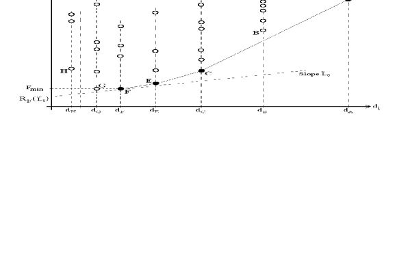
Fig. 4: Dominated hyperintervals are represented by white dots and non-dominated hyperintervals are represented by black dots.

It is important to notice that not all hyperintervals satisfying (17) are non-dominated. For example (see Fig. 4), the hyperinterval $D_{H}$ is dominated (with respect to any positive estimate of the Lipschitz constant $L$) by any of the hyperintervals $D_{G}$, $D_{F}$, or $D_{E}$. The hyperinterval $D_{G}$ is dominated by $D_{F}$. In fact, as it follows from (12), among several hyperintervals with the same sum of the function values at their vertices, larger hyperintervals dominate smaller ones with respect to any positive estimate of $L$. Finally, the hyperinterval $D_{B}$ is dominated either by the hyperinterval $D_{A}$ (for example, with respect to $\tilde{L}_{1}\geq\tilde{L}_{AC}$, where $\tilde{L}_{AC}$ corresponds to the slope of the line passed through the points $A$ and $C$ in Fig. 4), or by the hyperinterval $D_{C}$ (with respect to $\tilde{L}_{2}<\tilde{L}_{AC}$).

Note that if an estimate $\tilde{L}$ of the Lipschitz constant is chosen, it is easy to indicate the hyperinterval with the smallest lower bound of $f(x)$, that is, non-dominated hyperinterval with respect to $\tilde{L}$. To do this, it is sufficient to position a line with the slope $\tilde{L}$ below the set of dots in two-dimensional diagram representing hyperintervals of $\{D^{k}\}$, and then to shift it upwards. The first dot touched by the line indicates the desirable hyperinterval. For example, in Fig. 4 the hyperinterval $D_{F}$ represented by the point $F$ is non-dominated hyperinterval with respect to $\tilde{L}_{0}$, since over this hyperinterval $f(x)$ has the smallest lower bound $R_{F}(\tilde{L}_{0})$ for the given estimate $\tilde{L}_{0}$ of the Lipschitz constant.

Let us now examine various estimates of the Lipschitz constant $L$ from zero to infinity. When a small (close to zero) positive estimate of $L$ is chosen, an almost horizontal line is considered in two-dimensional diagram representing hyperintervals of a partition $\{D^{k}\}$. The dot with the smallest vertical coordinate $F_{min}$ (and the biggest horizontal coordinate if there are several such dots) is the first to be touched by this line (the case of the dot $F$ in Fig. 4). Therefore, hyperinterval (or hyperintervals) represented by this dot is non-dominated with respect to the chosen estimate of $L$, and, consequently, non-dominated in sense of Def. 2.2. Repeating such a procedure with higher estimates of the Lipschitz constant (that is, considering lines with higher slopes), all non-dominated hyperintervals can be identified. In Fig. 4 the hyperintervals represented by the dots $F$, $E$, $C$, and $A$ are non-dominated hyperintervals.

This procedure can be formalized in terms of the algorithm known as Jarvis march (or gift wrapping; see, e.g., [28]), which is an algorithm for identifying the convex hull of the dots. Thus, the following result identifying the set of non-dominated hyperintervals for a given partition $\{D^{k}\}$ has been proved.

Theorem 2.2.

Let each hyperinterval $D_{i}=[a_{i},b_{i}]\in\{D^{k}\}$ be represented by a dot with horizontal coordinate $d_{i}$ and vertical coordinate $F_{i}$ defined in (16). Then, non-dominated in sense of Def. 2.2 hyperintervals are located on the lower-right convex hull of the set of dots representing the hyperintervals.

We conclude this theoretical consideration by the following remark. As it has been shown in [31], the lengths of the main diagonals of hyperintervals generated by the new subdivision strategy from Section 2.1 are not arbitrary, contrarily to traditional diagonal schemes (see, e.g., [20, 24, 25, 26]). They are members of a sequence of values depending both on the size of the initial hypercube $D=[a,b]$ and on the number of executed subdivisions. In such a way, the hyperintervals of a current partition $\{D^{k}\}$ form several groups. Each group is characterized by the length of the main diagonals of hyperintervals within the group. In two-dimensional diagram ($d_{i},F_{i}$), where $d_{i}$ and $F_{i}$ are from (16), the hyperintervals from a group are represented by dots with the same horizontal coordinate $d_{i}$. For example, in Fig. 4 there are seven different groups of hyperintervals with the horizontal coordinates equal to $d_{A}$, $d_{B}$, $d_{C}$, $d_{E}$, $d_{F}$, $d_{G}$, and $d_{H}$. Note that some groups of a current partition can be empty (see, e.g., the group with the horizontal coordinate between $d_{H}$ and $d_{G}$ in Fig. 4). These groups correspond to diagonals which are not present in the current partition, but can be created (or were created) at the successive (previous) iterations of the algorithm.

It is possible to demonstrate (see [31]) that there exists a correspondence between the length of the main diagonal of a hyperinterval $D_{i}\in\{D^{k}\}$ and a non-negative integer number. This number indicates how many partitions have been performed starting from the initial hypercube $D$ to obtain the hyperinterval $D_{i}$. At each iteration $k\geq 1$ it can be considered as an index $l=l(k)$ of the corresponding group of hyperintervals having the same length of their main diagonals, where

$$0\leq q(k)\leq l(k)\leq Q(k)<+\infty$$ (18)

and $q(k)=q$ and $Q(k)=Q$ are indices corresponding to the groups of the largest and smallest hyperintervals of $\{D^{k}\}$, respectively. When the algorithm starts, there exists only one hyperinterval — the admissible region $D$ — which belongs to the group with the index $l=0$. In this case, both indices $q$ and $Q$ are equal to zero. When a hyperinterval $D_{i}\in\{D^{k}\}$ from a group $l^{\prime}=l^{\prime}(k)$ is subdivided, all three generated hyperintervals are placed into the group with the index $l^{\prime}+1$. Thus, during the work of the algorithm, diagonals of hyperintervals become smaller and smaller, while the corresponding indices of groups of hyperintervals grow consecutively starting from zero.

For example, in Fig. 4 there are seven non-empty groups of hyperintervals of a partition $\{D^{k}\}$ and one empty group. The index $q(k)$ (index $Q(k)$) corresponds to the group of the largest (smallest) hyperintervals represented in Fig. 4 by dots with the horizontal coordinate equal to $d_{A}$ ($d_{H}$). For Fig. 4 we have $Q(k)=q(k)+7$. The empty group has the index $l(k)=Q(k)-1$. Suppose that the hyperintervals $D_{A}$, $D_{H}$ and $D_{G}$ (represented in Fig. 4 by the dots $A$, $H$, and $G$, respectively) will be subdivided at the $k$-th iteration. In this case, the smallest index will remain the same, i.e., $q(k+1)=q(k)$, since the group of the largest hyperintervals will not be empty, while the biggest index will increase, i.e., $Q(k+1)=Q(k)+1$, since a new group of the smallest hyperintervals will be created. The previously empty group $Q(k)-1$ will be filled up by the new hyperintervals generated by partitioning the hyperinterval $D_{G}$ and will have the index $l(k+1)=Q(k+1)-2$.

3 New algorithm

In this section, a new algorithm for solving problem (1)–(3) is described. First, the new algorithm is presented and briefly commented. Then its convergence properties are analyzed.

The new algorithm is oriented on solving difficult multidimensional multiextremal problems. To accomplish this task, a two-phase approach consisting of explicitly defined global and local phases is proposed. It is well known that DIRECT also balances global and local information during its work. However, the local phase is too pronounced in this balancing. As has been already mentioned in Introduction, DIRECT executes too many function trials in regions of local optima and, therefore, manifests too slow convergence to the global minimizers when the objective function has many local minimizers.

In the new algorithm, when a sufficient number of subdivisions of hyperintervals near the current best point has been performed, the two-phase approach forces the new algorithm to switch to the exploration of large hyperintervals that could contain better solutions. Since many subdivisions have been executed around the current best point, its neighborhood contains only small hyperintervals and large ones can be located only far from it. Thus, the new algorithm balances global and local search in a more sophisticated way trying to provide a faster convergence to the global minimizers of difficult multiextremal functions.

Thus, the new algorithm consists of the following two phases: local improvement of the current best function value (local phase) and examination of large unexplored hyperintervals in pursuit of new attraction regions of deeper local minimizers (global phase). Each of these phases can consist of several iterations. During the local phase the algorithm tries to explore better the subregion around the current best point. This phase finishes when the following two conditions are verified: (i) an improvement on at least $1\%$ of the minimal function value is not more reached and (ii) a hyperinterval containing the current best point becomes the smallest one. After the end of the local phase the algorithm is switched to the global phase.

The global phase consists of subdividing mainly large hyperintervals, located possibly far from the current best point. It is performed until a function value improving the current minimal value on at least $1\%$ is obtained. When this happens, the algorithm switches to the local phase during which the obtained new solution is improved locally. During its work the algorithm can switch many times from the local phase to the global one. The algorithm stops when the number of generated trial points reaches the maximal allowed number.

We assume without loss of generality that the admissible region $D=[a,b]$ in (3) is an $N$-dimensional hypercube. Suppose that at the iteration $k\geq 1$ of the algorithm a partition $\{D^{k}\}$ of $D=[a,b]$ has been obtained by the partitioning procedure from (4)–(11). Suppose also that each hyperinterval $D_{i}\in\{D^{k}\}$ is represented by a dot in the two-dimensional diagram $(d_{i},F_{i})$, where $d_{i}$ and $F_{i}$ are from (16), and the groups of hyperintervals with the same length of their main diagonals are numerated by indices within a range from $q(k)$ up to $Q(k)$ from (18).

To describe the algorithm formally, we need the following additional designations:

$f_{min}(k)$ – the best function value (the term ‘record’ will be also used) found after $k-1$ iterations.

$x_{min}(k)$ – coordinates of $f_{min}(k)$.

$D_{min}(k)$ – the hyperinterval containing the point $x_{min}(k)$ (if $x_{min}(k)$ is a common vertex of several — up to $2^{N}$ — hyperintervals, then the smallest hyperinterval is considered).

$f_{min}^{prec}$ – the old record. It serves to memorize the record $f_{min}(k)$ at the start of the current phase (local or global). The value of $f_{min}^{prec}$ is updated when an improvement of the current record on at least $1\%$ is obtained.

$\xi$ – the parameter of the algorithm, $\xi\geq 0$. It prevents the algorithm from subdividing already well-explored small hyperintervals. If $D_{t}\in\{D^{k}\}$ is a non-dominated hyperinterval with respect to an estimate $\tilde{L}$ of the Lipschitz constant $L$, then this hyperinterval can be subdivided at the $k$-th iteration only if the following condition is satisfied

$$R_{t}(\tilde{L})\leq f_{min}(k)-\xi,$$ (19)

where the lower bound $R_{t}(\tilde{L})$ is calculated by formula (12). The value of $\xi$ can be set in different ways (see Section 4).

$T_{max}$ – the maximal allowed number of trial points that the algorithm may generate. The algorithm stops when the number of generated trial points reaches $T_{max}$. During the course of the algorithm the satisfaction of this termination criterion is verified after every subdivision of a hyperinterval.

$Lcounter$, $Gcounter$ – the counters of iterations executed during the current local and global phases, respectively.

$p(k)$ – the index of the group the hyperinterval $D_{min}(k)$ belongs to. Notice that the inequality $q(k)\leq p(k)\leq Q(k)$ is satisfied for any iteration number $k$. Since both local and global phases can embrace more than one iteration, the index $p(k)$ (as well as the indices $q(k)$ and $Q(k)$) can change (namely, increase) during these phases. Note also that the group $p(k)$ can be different from the groups containing hyperintervals with the smallest sum of the objective function values at their vertices (see two groups of hyperintervals represented in Fig. 4 by the horizontal coordinates equal to $d_{G}$ and $d_{F}$). Moreover, the hyperinterval $D_{min}(k)$ is not represented necessarily by the ‘lowest’ point from the group $p(k)$ in the two-dimensional diagram $(d_{i},F_{i})$ – even if the current best function value is obtained at a vertex of $D_{min}(k)$, the function value at the other vertex can be too high and the sum of these two values can be greater than the corresponding value of another hyperinterval from the group $p(k)$.

$p^{\prime}$ – the index of the group containing the hyperinterval $D_{min}(k)$ at the start of the current phase (local or global). Hyperintervals from the groups with indices greater than $p^{\prime}$ are not considered when non-dominated hyperintervals are looked for. Whereas the index $p(k)$ can assume different values during the current phase, the index $p^{\prime}$ remains, as a rule, invariable. It is changed only when it violates the left part of condition (18). This can happen when groups with the largest hyperintervals disappear and, therefore, the index $q(k)$ increases and becomes equal to $p^{\prime}$. In this case, the index $p^{\prime}$ increases jointly with $q(k)$.

$p^{\prime\prime}$ – the index of the group immediately preceding the group $p^{\prime}$, i.e., $p^{\prime\prime}=p^{\prime}-1$. This index is used within the local phase and can increase if $q(k)$ increases during this phase.

$r^{\prime}$ – the index of the middle group of hyperintervals between the groups $p^{\prime}$ and $q(k)$, i.e., $r^{\prime}=\lceil(q(k)+p^{\prime})/2\rceil$. This index is used within the global phase as a separator between the groups of large and small hyperintervals. It can increase if $q(k)$ increases during this phase.

To clarify the introduced group indices, let us consider an example of a partition $\{D^{k}\}$ represented by the two-dimensional diagram in Fig. 4. Let us suppose that the index $q(k)$ of the group of the largest hyperintervals corresponding to the points with the horizontal coordinate $d_{A}$ in Fig. 4 is equal to 10. The index $Q(k)$ of the group of the smallest hyperintervals with the main diagonals equal to $d_{H}$ (see Fig. 4) is equal to $Q(k)=q(k)+7=17$. Let us also assume that the hyperinterval $D_{min}(k)$ belongs to the group of hyperintervals with the main diagonals equal to $d_{G}$ (see Fig. 4). In this case, the index $p(k)$ is equal to 15 and the index $p^{\prime}$ is equal to 15 too. The index $p^{\prime\prime}=15-1=14$ and it corresponds to the group of hyperintervals represented in Fig. 4 by the dots with the horizontal coordinate $d_{F}$. Finally, the index $r^{\prime}=\lceil(10+15)/2\rceil=13$ and it corresponds to hyperintervals with the main diagonals equal to $d_{E}$. The indices $p^{\prime}$, $p^{\prime\prime}$, and $r^{\prime}$ can change only if the index $q(k)$ increases. Otherwise, they remain invariable during the iterations of the current phase (local or global). At the same time, the index $p(k)$ can change at every iteration, as soon as a new best function value belonging to a hyperinterval of a group different from $p(k)$ is obtained.

Now we are ready to present a formal scheme of the new algorithm.

Step 1: Initialization.

Set the current iteration number $k:=1$, the current record $f_{min}(k):=\min\{f(a),f(b)\}$ where $a$ and $b$ are from (3). Set group indices $q(k):=Q(k):=p(k):=0$.

Step 2: Local Phase.

Memorize the current record $f_{min}^{prec}:=f_{min}(k)$ and perform the following steps:

Step 2.1.

Set $Lcounter:=1$ and fix the group index $p^{\prime}:=p(k)$.

Step 2.2.

Set $p^{\prime\prime}:=\max\{p^{\prime}-1,q(k)\}$.

Step 2.3.

Determine non-dominated hyperintervals considering only groups of hyperintervals with the indices from $q(k)$ up to $p^{\prime\prime}$. Subdivide those non-dominated hyperintervals which satisfy inequality (19). Set $k:=k+1$.

Step 2.4.

Set $Lcounter:=Lcounter+1$ and check whether $Lcounter\leq N$. If this is the case, then go to Step 2.2. Otherwise, go to Step 2.5.

Step 2.5.

Set $p^{\prime}=\max\{p^{\prime},q(k)\}$. Determine non-dominated hyperintervals considering only groups of hyperintervals with the indices from $q(k)$ up to $p^{\prime}$. Subdivide those non-dominated hyperintervals which satisfy inequality (19). Set $k:=k+1$.

Step 3: Switch.

If condition

$$f_{min}(k)\leq f_{min}^{prec}-0.01|f_{min}^{prec}|$$ (20)

is satisfied, then go to Step 2 and repeat the local phase with the new obtained value of the record $f_{min}(k)$. Otherwise, if the hyperinterval $D_{min}(k)$ is not the smallest one, or the current partition of $D$ consists only of hyperintervals with equal diagonals (i.e., $p(k)<Q(k)$ or $q(k)=Q(k)$), then go to Step 2.1 and repeat the local phase with the old record $f_{min}^{prec}$.

If the obtained improvement of the best function value is not sufficient to satisfy (20) and $D_{min}(k)$ is the smallest hyperinterval of the current partition (i.e., all the following inequalities – (20), $p(k)<Q(k)$, and $q(k)=Q(k)$ — fail), then go to Step 4 and perform the global phase.

Step 4: Global Phase.

Memorize the current record $f_{min}^{prec}:=f_{min}(k)$ and perform the following steps:

Step 4.1.

Set $Gcounter:=1$ and fix the group index $p^{\prime}:=p(k)$.

Step 4.2.

Set $p^{\prime}=\max\{p^{\prime},q(k)\}$ and calculate the ‘middle’ group index $r^{\prime}=\lceil(q(k)+p^{\prime})/2\rceil$.

Step 4.3.

Determine non-dominated hyperintervals considering only groups of hyperintervals with the indices from $q(k)$ up to $r^{\prime}$. Subdivide those non-dominated hyperintervals which satisfy inequality (19). Set $k:=k+1$.

Step 4.4.

If condition (20) is satisfied, then go to Step 2 and perform the local phase with the new obtained value of the record $f_{min}(k)$. Otherwise, go to Step 4.5.

Step 4.5.

Set $Gcounter:=Gcounter+1$; check whether $Gcounter\leq 2^{N+1}$. If this is the case, then go to Step 4.2. Otherwise, go to Step 4.6.

Step 4.6.

Set $p^{\prime}=\max\{p^{\prime},q(k)\}$. Determine non-dominated hyperintervals considering only groups of hyperintervals with the indices from $q(k)$ up to $p^{\prime}$. Subdivide those non-dominated hyperintervals which satisfy inequality (19). Set $k:=k+1$.

Step 4.7.

If condition (20) is satisfied, then go to Step 2 and perform the local phase with the new obtained value of the record $f_{min}(k)$. Otherwise, go to Step 4.1: update the value of the group index $p^{\prime}$ and repeat the global phase with the old record $f_{min}^{prec}$.

Let us give a few comments on the introduced algorithm. It starts from the local phase. In the course of this phase, it subdivides non-dominated hyperintervals with the main diagonals greater than the main diagonal of $D_{min}(k)$ (i.e., from the groups with the indices from $q(k)$ up to $p^{\prime}$; see Steps 2.1 – 2.4). This operation is repeated $N$ times, where $N$ is the problem dimension from (3). Remind that during each subdivision of a hyperinterval by the scheme (4) – (11) only one side of the hyperinterval (namely, the longest side given by formula (7)) is partitioned. Thus, performing $N$ iterations of the local phase eventually subdivides all $N$ sides of hyperintervals around the current best point. At the last, $(N+1)$-th, iteration of the local phase (see Step 2.5) hyperintervals with the main diagonal equal to $D_{min}(k)$ are considered too. In such a way, the hyperinterval containing the current best point can be partitioned too.

Thus, either the current record is improved, or the hyperinterval providing this record becomes smaller. If the conditions of switching to the global phase (see Step 3) are not satisfied, the local phase is repeated. Otherwise, the algorithm switches to the global phase, avoiding unnecessary evaluations of $f(x)$ within already well explored subregions.

During the global phase the algorithm searches for better new minimizers. It performs series of loops (see Steps 4.1 – 4.7) while a non-trivial improvement of the best function value is not obtained, i.e., condition (20) is not satisfied. Within a loop of the global phase the algorithm performs a substantial number of subdivisions of large hyperintervals located far from the current best point, namely, hyperintervals from the groups with the indices from $q(k)$ up to $r^{\prime}$ (see Steps 4.2 – 4.5). Since each trial point can belong up to $2^{N}$ hyperintervals, the number of subdivisions should not be smaller than $2^{N}$. The value of this number equal to $2^{N+1}$ has been chosen because it provided a good performance of the algorithm in our numerical experiments.

Note that the situation when the current best function value is improved but the amount of this improvement is not sufficient to satisfy (20), can be verified at the end of a loop of the global phase (see Step 4.7). In this case, the algorithm is not switched to the local phase. It proceeds with the next loop of the global phase, eventually updating the index $p^{\prime}$ (see Step 4.1) but non updating the old record $f_{min}^{prec}$.

Let us now study convergence properties of the new algorithm during minimization of the function $f(x)$ from (1)–(3) when the maximal allowed number of generated trial points $T_{max}$ is equal to infinity. In this case, the algorithm does not stop (the number of iterations $k$ goes to infinity) and an infinite sequence of trial points $\{x^{j(k)}\}$ is generated. The following theorem establishes the so-called ‘everywhere dense’ convergence of the new algorithm.

Theorem 3.1.

For any point $x\in D$ and any $\delta>0$ there exist an iteration number $k(\delta)\geq 1$ and a point $x^{\prime}\in\{x^{j(k)}\}$, $k>k(\delta)$, such that $\|x-x^{\prime}\|<\delta$.

Proof.

Trial points generated by the new algorithm are vertices of the main diagonals of hyperintervals. Due to (4)–(11), every subdivision of a hyperinterval produces three new hyperintervals with the volume equal to a third of the volume of the subdivided hyperinterval and the proportionally smaller main diagonals. Thus, fixed a positive value of $\delta$, it is sufficient to prove that after a finite number of iterations $k(\delta)$ the largest hyperinterval of the current partition of $D$ will have the main diagonal smaller than $\delta$. In such a case, in $\delta$-neighborhood of any point of $D$ there will exist at least one trial point generated by the algorithm.

To see this, let us fix an iteration number $k^{\prime}$ and consider the group $q(k^{\prime})$ of the largest hyperintervals of a partition $\{D^{k^{\prime}}\}$. As it can be seen from the scheme of the algorithm, for any $k^{\prime}\geq 1$ this group is taken into account when non-dominated hyperintervals are looked for. Moreover, a hyperinterval $D_{t}\in\{D^{k^{\prime}}\}$ from this group having the smallest sum of the objective function values at its vertices is partitioned at each iteration $k\geq 1$ of the algorithm. This happens because there always exists a sufficiently large estimate $L_{\infty}$ of the Lipschitz constant $L$ such that the hyperinterval $D_{t}$ is a non-dominated hyperinterval with respect to $L_{\infty}$ and condition (19) is satisfied for the lower bound $R_{t}(L_{\infty})$ (see Fig. 4). Three new hyperintervals generated during the subdivision of $D_{t}$ by using the strategy (4)–(11) are inserted into the group with the index $q(k^{\prime})+1$. Hyperintervals of the group $q(k^{\prime})+1$ have the volume equal to a third of the volume of hyperintervals of the group $q(k^{\prime})$.

Since each group contains only finite number of hyperintervals, after a sufficiently large number of iterations $k>k^{\prime}$ all hyperintervals of the group $q(k^{\prime})$ will be subdivided. The group $q(k^{\prime})$ will become empty and the index of the group of the largest hyperintervals will increase, i.e., $q(k)=q(k^{\prime})+1$. Such a procedure will be repeated with a new group of the largest hyperintervals. So, when the number of iterations grows, the index $q(k)$ increases and due to (18) the index $Q(k)$ increases too. This means, that there exists a finite number of iterations $k(\delta)$ such that after performing $k(\delta)$ iterations of the algorithm the largest hyperinterval of the current partition $\{D^{k(\delta)}\}$ will have the main diagonal smaller than $\delta$.   ∎

4 Numerical results

In this section, we present results performed to compare the new algorithm with two methods belonging to the same class: the original DIRECT algorithm from [18] and its locally-biased modification DIRECTl  from [10, 11]. The implementation of these two methods described in [8, 10] and downloadable from [9] has been used in all the experiments.

To execute a numerical comparison, we need to define the parameter $\xi$ of the algorithm from (19). This parameter can be set either independently from the current record $f_{min}(k)$, or in a relation with it. Since the objective function $f(x)$ is supposed to be “black-box”, it is not possible to know a priori which of these two ways is better.

In DIRECT [18], where a similar parameter is used, a value $\xi$ related to the current minimal function value $f_{min}(k)$ is fixed as follows

$$\xi=\varepsilon|f_{min}(k)|,\hskip 8.53581pt\varepsilon\geq 0.$$ (21)

The choice of $\varepsilon$ between $10^{-3}$ and $10^{-7}$ has demonstrated good results for DIRECT on a set of test functions (see [18]). Later formula (21) has been used by many authors (see, e.g., [3, 6, 10, 11, 13]) and also has been realized in the implementation of DIRECT (see [8, 10]) taken for numerical comparison with the new algorithm. Since the value of $\varepsilon=10^{-4}$ recommended in [18] has produced the most robust results for DIRECT (see, e.g., [10, 11, 13, 18]), exactly this value was used in (21) for DIRECT in our numerical experiments. In order to have comparable results, the same formula (21) and $\varepsilon=10^{-4}$ were used in the new algorithm too.

The global minimizer $x^{*}\in D$ was considered to be found when an algorithm generated a trial point $x^{\prime}$ inside a hyperinterval with a vertex $x^{*}$ and the volume smaller than the volume of the initial hyperinterval $D=[a,b]$ multiplied by an accuracy coefficient $\Delta$, $0<\Delta\leq 1$, i.e.,

$$|x^{\prime}(i)-x^{*}(i)|\leq\sqrt[N]{\Delta}(b(i)-a(i)),\hskip 8.53581pt1\leq i\leq N,$$ (22)

where $N$ is from (3). This condition means that, given $\Delta$, a point $x^{\prime}$ satisfies (22) if the hyperinterval with the main diagonal $[x^{\prime},x^{*}]$ and the sides proportional to the sides of the initial hyperinterval $D=[a,b]$ has a volume at least $\Delta^{-1}$ times smaller than the volume of $D$. Note that if in (22) the value of $\Delta$ is fixed and the problem dimension $N$ increases, the length of the diagonal of the hyperinterval $[x^{\prime},x^{*}]$ increases too. In order to avoid this undesirable growth, the value of $\Delta$ was progressively decreased when the problem dimension increased.

We stopped the algorithm either when the maximal number of trials $T_{max}$ was reached, or when condition (22) was satisfied. Note that such a type of stopping criterion is acceptable only when the global minimizer $x^{*}$ is known, i.e., for the case of test functions. When a real “black-box” objective function is minimized and global minimization algorithms have an internal stopping criterion, they execute a number of iterations (that can be very high) after a ‘good’ estimate of $f^{*}$ has been obtained in order to demonstrate a ‘goodness’ of the found solution (see, e.g., [14, 26, 33]).

Table 1: Number of trial points for test functions used in [18].

Function	$N$	$D=[a,b]$	$\Delta$	DIRECT	DIRECTl	New
Shekel 5	4	$[0,10]^{4}$	$10^{-6}$	57	53	208
Shekel 7	4	$[0,10]^{4}$	$10^{-6}$	53	45	1465
Shekel 10	4	$[0,10]^{4}$	$10^{-6}$	53	45	1449
Hartman 3	3	$[0,1]^{3}$	$10^{-6}$	113	79	137
Hartman 6	6	$[0,1]^{6}$	$10^{-7}$	144	78	4169
Branin RCOS	2	$[-5,10]\times[0,15]$	$10^{-4}$	41	31	76
Goldstein and Price	2	$[-2,2]^{2}$	$10^{-4}$	37	29	99
Six-Hump Camel	2	$[-3,3]\times[-2,2]$	$10^{-4}$	105	127	128
Shubert	2	$[-8,10]^{2}$	$10^{-4}$	19	15	59

In the first series of experiments, test functions from [5] and [36] were used because in [10, 11, 18] DIRECT and DIRECTl have been tested on these functions. It can be seen from Table 1 that both methods DIRECT and DIRECTl have executed a very small amount of trials until they generated a point in a neighborhood (22) of a global minimizer. For example, condition (22) was satisfied for the six-dimensional Hartman’s function after 78 (144) trials performed by DIRECTl (DIRECT). Such a small number of trials is explained by a simple structure of the function. We observe, in accordance with [34], that the test functions from [5] used in [18] are not suitable for testing global optimization methods. These functions are characterized by a small chance to miss the region of attraction of the global minimizer (see [34]). Usually, when a real difficult “black-box” function of high dimension is minimized, the number of trials that it is necessary to execute to place a trial point in the neighborhood of the global minimizer is significantly higher. The algorithm proposed in this paper is oriented on such a type of functions. It tries to perform a good examination of the admissible region in order to reduce the risk of missing the global solution. Therefore, for simple test functions of Table 1 and the stopping rule (22) it generated more trial points than DIRECT or DIRECTl.

Hence, more sophisticated test problems are required for carrying out numerical comparison among global optimization algorithms (see also the related discussion in [19]).

Many difficult global optimization tests can be taken from real-life applications (see, e.g., [7] and bibliographic references within it). But the lack of comprehensive information (such as number of local minima, their locations, attraction regions, local and global values, ecc.) describing these tests creates an obstacle in verifying efficiency of the algorithms. Very frequently it is also difficult to fix properly many correlated parameters determining some test functions because often the sense of these parameters is not intuitive, especially in high dimensions. Moreover, tests may differ too much one from another and as a result it is not possible to have many test functions with similar properties. Therefore, the use of randomly-generated classes of test functions having similar properties can be a reasonable solution for a satisfactory comparison.

Thus, in our numerical experiments we used the GKLS-generator described in [12] (and free-downloadable from http://wwwinfo.deis.unical.it/ $\tilde{}$yaro/GKLS.html). It generates classes of multidimensional and multiextremal test functions with known local and global minima. The procedure of generation consists of defining a convex quadratic function (paraboloid) systematically distorted by polynomials. Each test class provided by the generator includes 100 functions and is defined only by the following five parameters:

$N$ – problem dimension;

$M$ – number of local minima;

$f^{*}$ – value of the global minimum;

$\rho^{*}$ – radius of the attraction region of the global minimizer;

$r^{*}$ – distance from the global minimizer to the vertex of the paraboloid.

The other necessary parameters are chosen randomly by the generator for each test function of the class. Note, that the generator produces always the same test classes for a given set of the user-defined parameters allowing one to perform repeatable numerical experiments.

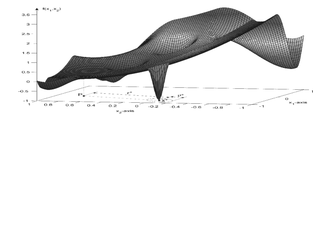
Fig. 5: An example of the two-dimensional function from the GKLS test class.

By changing the user-defined parameters, classes with different properties can be created. For example, fixed dimension of the functions and number of local minima, a more difficult class can be created either by shrinking the attraction region of the global minimizer, or by moving the global minimizer far away from the paraboloid vertex.

For conducting numerical experiments, we used eight GKLS classes of continuously differentiable test functions of dimensions $N=2$, 3, 4, and 5. The number of local minima $M$ was equal to 10 and the global minimum value $f^{*}$ was equal to $-1.0$ for all classes (these values are default settings of the generator). For each particular problem dimension $N$ we considered two test classes: a simple class and a difficult one. The difficulty of a class was increased either by decreasing the radius $\rho^{*}$ of the attraction region of the global minimizer (as for two- and five-dimensional classes), or by increasing the distance $r^{*}$ from the global minimizer $x^{*}$ to the paraboloid vertex $P$ (three- and four-dimensional classes).

In Fig. 5, an example of a test function from the following continuously differentiable GKLS class is given: $N=2$, $M=10$, $f^{*}=-1$, $\rho^{*}=0.10$, and $r^{*}=0.90$. This function is defined over the region $D=[-1,1]^{2}$ and its number is 87 in the given test class. The randomly generated global minimizer of this function is $x^{*}=(-0.767,-0.076)$ and the coordinates of $P$ are $(-0.489,0.780)$. Results for the whole class to which the function from Fig. 5 belongs to are given in Tables 2 and 3 on the second line.

We stopped algorithms either when the maximal number of trials $T_{max}$ equal to 1 000 000 was reached, or when condition (22) was satisfied. To describe experiments, we introduce the following designations:

$T_{s}$ – the number of trials performed by the method under consideration to solve the problem number $s$, $1\leq s\leq 100$, of a fixed test class. If the method was not able to solve a problem $j$ in less than $T_{max}$ function evaluations, $T_{j}$ equal to $T_{max}$ was taken.

$m_{s}$ – the number of hyperintervals generated to solve the problem $s$.

The following four criteria were used to compare the methods.

Criterion C1. Number of trials $T_{s^{*}}$ required for a method to satisfy condition (22) for all 100 functions of a particular test class, i.e.,

$$T_{s^{*}}=\max_{1\leq s\leq 100}T_{s},\hskip 14.22636pts^{*}=\arg\max_{1\leq s\leq 100}T_{s}.$$ (23)

Criterion C2. The corresponding number of hyperintervals, $m_{s^{*}}$, generated by the method, where $s^{*}$ is from (23).

Criterion C3. Average number of trials $T_{avg}$ performed by the method during minimization of all 100 functions from a particular test class, i.e.,

$$T_{avg}=\frac{1}{100}\sum_{s=1}^{100}T_{s}.$$ (24)

Criterion C4. Number $p$ (number $q$) of functions from a class for which DIRECT or DIRECTl executed less (more) function evaluations than the new algorithm. If $T_{s}$ is the number of trials performed by the new algorithm and $T_{s}^{\prime}$ is the corresponding number of trials performed by a competing method, $p$ and $q$ are evaluated as follows

$$p=\sum_{s=1}^{100}\delta_{s}^{\prime},\hskip 14.22636pt\delta_{s}^{\prime}=\left\{\begin{array}[]{ll}1,&T_{s}^{\prime}<T_{s},\\ 0,&{\rm otherwise}.\end{array}\right.$$ (25)

$$q=\sum_{s=1}^{100}\delta_{s},\hskip 14.22636pt\delta_{s}=\left\{\begin{array}[]{ll}1,&T_{s}<T_{s}^{\prime},\\ 0,&{\rm otherwise}.\end{array}\right.$$ (26)

If $p+q<100$ then both the methods under consideration solve the remaining ($100-p-q$) problems with the same number of function evaluations.

Note that results based on Criteria C1 and C2 are mainly influenced by minimization of the most difficult functions of a class. Criteria C3 and C4 deal with average data of a class.

Criterion C1 is of the fundamental importance for the methods comparison on the whole test class because it shows how many trials it is necessary to execute to solve all the problems of a class. Thus, it represents the worst case results of the given method on the fixed class.

At the same time, the number of generated hyperintervals (Criterion C2) provides an important characteristic of any partition algorithm for solving (1)–(3). It reflects indirectly the degree of qualitative examination of $D$ during the search for a global minimum. The greater is this number, the more information about the admissible domain is available and, therefore, the smaller should be the risk to miss the global minimizer. However, algorithms should not generate many redundant hyperintervals since this slows down the search and is therefore a disadvantage of the method.

Let us first compare the three methods on Criteria C1 and C2. Results of numerical experiments with eight GKLS tests classes are shown in Tables 2 and 3. The accuracy coefficient $\Delta$ from (22) is given in the second column of the tables. Table 2 reports the maximal number of trials required for satisfying condition (22) for a half of the functions of a particular class (columns “50%”) and for all 100 function of the class (columns “100%”). The notation ‘$>$ 1 000 000 $(j)$’ means that after 1 000 000 function evaluations the method under consideration was not able to solve $j$ problems. The corresponding numbers of generated hyperintervals are indicated in Table 3. Since DIRECT and DIRECTl use during their work the central-sampling partition strategy, the number of generated trial points and the number of generated hyperintervals coincide for these methods.

Note that on a half of test functions from each class (which were the most simple for each method with respect to the other functions of the class) the new algorithm manifested a good performance with respect to DIRECT and DIRECTl in terms of the number of generated trial points (see columns “50%” in Table 2). When all the functions were taken in consideration (and, consequently, difficult functions of the class were considered too), the number of trials produced by the new algorithm was much fewer in comparison with two other methods (see columns “100%” in Table 2), ensuring at the same time a substantial examination of the admissible domain (see Table 3).

Table 2: Number of trial points for GKLS test functions (Criterion C1).

$N$	$\Delta$	Class		50%			100%
		$r^{*}$	$\rho^{*}$	DIRECT	DIRECTl	New	DIRECT	DIRECTl	New
2	$10^{-4}$	.90	.20	111	152	166	1159	2318	403
2	$10^{-4}$	.90	.10	1062	1328	613	3201	3414	1809
3	$10^{-6}$	.66	.20	386	591	615	12507	13309	2506
3	$10^{-6}$	.90	.20	1749	1967	1743	$>$1000000 (4)	29233	6006
4	$10^{-6}$	.66	.20	4805	7194	4098	$>$1000000 (4)	118744	14520
4	$10^{-6}$	.90	.20	16114	33147	15064	$>$1000000 (7)	287857	42649
5	$10^{-7}$	.66	.30	1660	9246	3854	$>$1000000 (1)	178217	33533
5	$10^{-7}$	.66	.20	55092	126304	24616	$>$1000000 (16)	$>$1000000 (4)	93745

Table 3: Number of hyperintervals for GKLS test functions (Criterion C2).

$N$	$\Delta$	Class		50%			100%
		$r^{*}$	$\rho^{*}$	DIRECT	DIRECTl	New	DIRECT	DIRECTl	New
2	$10^{-4}$	.90	.20	111	152	269	1159	2318	685
2	$10^{-4}$	.90	.10	1062	1328	1075	3201	3414	3307
3	$10^{-6}$	.66	.20	386	591	1545	12507	13309	6815
3	$10^{-6}$	.90	.20	1749	1967	5005	$>$1000000	29233	17555
4	$10^{-6}$	.66	.20	4805	7194	15145	$>$1000000	118744	73037
4	$10^{-6}$	.90	.20	16114	33147	68111	$>$1000000	287857	211973
5	$10^{-7}$	.66	.30	1660	9246	21377	$>$1000000	178217	206323
5	$10^{-7}$	.66	.20	55092	126304	177927	$>$1000000	$>$1000000	735945

In our opinion, the impossibility of DIRECT to determine global minimizers of several test functions is related to the following fact. DIRECT found quickly the vertex of the paraboloid (at which the function value is set by default equal to 0) used for determining GKLS test functions. Hence, the parameter $\xi$ was very close to zero (due to (21)) and condition similar to (19) was satisfied for almost all small hyperintervals. Moreover, many small hyperintervals around the paraboloid vertex with function values close one to another and to the current minimal value were created. In such a situation, DIRECT subdivided many of these hyperintervals. Thus, at each iteration DIRECT partitioned a large amount of small hyperintervals and, therefore, was not able to go out from the attraction region of the paraboloid vertex.

Table 4: Number of trial points for shifted GKLS test functions (Criterion C1).

$N$	$\Delta$	Class		50%			100%
		$r^{*}$	$\rho^{*}$	DIRECT	DIRECTl	New	DIRECT	DIRECTl	New
2	$10^{-4}$	.90	.20	111	146	165	1087	1567	403
2	$10^{-4}$	.90	.10	911	1140	508	2973	2547	1767
3	$10^{-6}$	.66	.20	364	458	606	6292	10202	1912
3	$10^{-6}$	.90	.20	1485	1268	1515	14807	28759	4190
4	$10^{-6}$	.66	.20	4193	4197	3462	37036	95887	14514
4	$10^{-6}$	.90	.20	14042	24948	11357	251801	281013	32822
5	$10^{-7}$	.66	.30	1568	3818	3011	102869	170709	15343
5	$10^{-7}$	.66	.20	32926	116025	15071	454925	$>1000000(1)$	77981

Table 5: Number of hyperintervals for shifted GKLS test functions (Criterion C2).

$N$	$\Delta$	Class		50%			100%
		$r^{*}$	$\rho^{*}$	DIRECT	DIRECTl	New	DIRECT	DIRECTl	New
2	$10^{-4}$	.90	.20	111	146	281	1087	1567	685
2	$10^{-4}$	.90	.10	911	1140	905	2973	2547	3227
3	$10^{-6}$	.66	.20	364	458	1585	6292	10202	5337
3	$10^{-6}$	.90	.20	1485	1268	4431	14807	28759	12949
4	$10^{-6}$	.66	.20	4193	4197	14961	37036	95887	73049
4	$10^{-6}$	.90	.20	14042	24948	57111	251801	281013	181631
5	$10^{-7}$	.66	.30	1568	3818	17541	102869	170709	106359
5	$10^{-7}$	.66	.20	32926	116025	108939	454925	$>1000000$	685173

Table 6: Improvement obtained by the new algorithm in terms of Criterion C1.

$N$	$\Delta$	Class		GKLS		Shifted GKLS
		$r^{*}$	$\rho^{*}$	DIRECT/New	DIRECTl/New	DIRECT/New	DIRECTl/New
2	$10^{-4}$	.90	.20	2.88	5.75	2.70	3.89
2	$10^{-4}$	.90	.10	1.77	1.89	1.68	1.44
3	$10^{-6}$	.66	.20	4.99	5.31	3.29	5.34
3	$10^{-6}$	.90	.20	$>$166.50	4.87	3.53	6.86
4	$10^{-6}$	.66	.20	$>$68.87	8.18	2.55	6.61
4	$10^{-6}$	.90	.20	$>$23.45	6.75	7.67	8.56
5	$10^{-7}$	.66	.30	$>$29.82	5.31	6.70	11.13
5	$10^{-7}$	.66	.20	$>$10.67	$>$10.67	5.83	$>$12.82

Since DIRECTl at each iteration subdivides only one hyperinterval among all hyperintervals with the same function value, it was able to determine some other local minimizers (and the global minimizer too) in the given maximal number of trials $T_{max}$. So, DIRECTl overcame the stagnation of the search around the paraboloid vertex. But due to the locally-biased character of DIRECTl, it spent too much trials exploring various local minimizers which were not global. For this reason, DIRECTl was unable to find the global minimizers of four difficult five-dimensional functions.

In order to avoid stagnation of DIRECT near the paraboloid vertex and to put DIRECT and DIRECTl in a more advantageous situation, we shifted all generated functions, adding to their values the constant 2. In such a way the value of each function at the paraboloid vertex became equal to $2$ (and the global minimum value $f^{*}$ was increased by 2, i.e., became equal to $1$). Results of numerical experiments with shifted GKLS classes (defined in the rest by the same parameters) are reported in Tables 4 and 5. Note that in this case DIRECT has found the global solutions of all problems. DIRECTl has not found the global minimizer of one five-dimensional function. It can be seen from Tables 4 and 5 that also on these tests classes the new algorithm has manifested its superiority with respect to DIRECT and DIRECTl in terms of the number of generated trial points (Criterion C1).

Table 6 summarizes (based on the data from Tables 2 – 5) results (in terms of Criterion C1) of numerical experiments performed on 1600 test functions from GKLS and shifted GKLS continuously differentiable classes. It represents the ratio between the maximal number of trials performed by DIRECT and DIRECTl with respect to the corresponding number of trials performed by the new algorithm. It can be seen from Table 6 that the new method outperforms both competitors significantly on the given test classes when Criteria C1 and C2 are considered.

Table 7: Average number of trial points for GKLS test functions (Criterion C3).

$N$	$\Delta$	Class		DIRECT	DIRECTl	New	Improvement
		$r^{*}$	$\rho^{*}$				DIRECT/New	DIRECTl/New
2	$10^{-4}$	.90	.20	198.89	292.79	176.25	1.13	1.66
2	$10^{-4}$	.90	.10	1063.78	1267.07	675.74	1.57	1.88
3	$10^{-6}$	.66	.20	1117.70	1785.73	735.76	1.52	2.43
3	$10^{-6}$	.90	.20	$>$42322.65	4858.93	2006.82	$>$21.09	2.42
4	$10^{-6}$	.66	.20	$>$47282.89	18983.55	5014.13	$>$9.43	3.79
4	$10^{-6}$	.90	.20	$>$95708.25	68754.02	16473.02	$>$5.81	4.17
5	$10^{-7}$	.66	.30	$>$16057.46	16758.44	5129.85	$>$3.13	3.27
5	$10^{-7}$	.66	.20	$>$217215.58	$>$269064.35	30471.83	$>$7.13	$>$8.83

Table 8: Average number of trial points for shifted GKLS test functions (Criterion C3).

$N$	$\Delta$	Class		DIRECT	DIRECTl	New	Improvement
		$r^{*}$	$\rho^{*}$				DIRECT/New	DIRECTl/New
2	$10^{-4}$	.90	.20	185.83	249.25	173.43	1.07	1.44
2	$10^{-4}$	.90	.10	953.34	1088.13	609.36	1.56	1.79
3	$10^{-6}$	.66	.20	951.04	1434.33	683.73	1.39	2.10
3	$10^{-6}$	.90	.20	2226.36	3707.85	1729.55	1.29	2.14
4	$10^{-6}$	.66	.20	7110.72	14523.45	4388.22	1.62	3.31
4	$10^{-6}$	.90	.20	24443.60	56689.06	12336.56	1.98	4.60
5	$10^{-7}$	.66	.30	5876.99	10487.80	4048.31	1.45	2.59
5	$10^{-7}$	.66	.20	59834.38	$>$182385.59	19109.20	3.13	$>$9.54

Let us now compare the three methods using Criteria C3 and C4. Tables 7 and 8 report the average numbers of trials performed during minimization of all 100 functions from the same GKLS and shifted GKLS classes, respectively (Criterion C3). The columns “Improvement” of these tables represent the ratios between the average numbers of trials performed by DIRECT and DIRECTl with respect to the corresponding numbers of trials performed by the new algorithm. The symbol ‘$>$’ reflects the situation when not all functions of a class were successfully minimized by the method under consideration in sense of condition (22). This means that the method stopped when $T_{max}$ trials have been executed during minimization of several functions of this particular test class. In these cases, the value of $T_{max}$ equal to 1 000 000 was used in calculations of the average value in (24), providing in such a way a lower estimate of the average. As it can be seen from Tables 7 and 8, the new method outperforms DIRECT and DIRECTl also on Criterion C3.

Table 9: Comparison between the new algorithm and DIRECT and DIRECTl in terms of Criterion C4.

$N$	$\Delta$	Class		GKLS		Shifted GKLS
		$r^{*}$	$\rho^{*}$	DIRECT : New	DIRECTl : New	DIRECT : New	DIRECTl : New
2	$10^{-4}$	.90	.20	61 : 39	52 : 47	61 : 38	54 : 46
2	$10^{-4}$	.90	.10	36 : 64	23 : 77	37 : 63	23 : 77
3	$10^{-6}$	.66	.20	66 : 34	54 : 46	65 : 35	62 : 38
3	$10^{-6}$	.90	.20	58 : 42	51 : 49	56 : 44	54 : 46
4	$10^{-6}$	.66	.20	51 : 49	37 : 63	50 : 50	44 : 56
4	$10^{-6}$	.90	.20	47 : 53	42 : 58	46 : 54	43 : 57
5	$10^{-7}$	.66	.30	66 : 34	26 : 74	67 : 33	42 : 58
5	$10^{-7}$	.66	.20	34 : 66	27 : 73	32 : 68	32 : 68

Finally, results of comparison between the new algorithm and its two competitors in terms of Criterion C4 are reported in Table 9. This table shows how often the new algorithm was able to minimize each of 100 functions of a class with a smaller number of trials with respect to DIRECT or DIRECTl. The notation ‘$p$ : $q$’ means that among 100 functions of a particular test class there are $p$ functions for which DIRECT (or DIRECTl) spent less function trials than the new algorithm and $q$ functions for which the new algorithm generated fewer trial points with respect to DIRECT (or DIRECTl) ($p$ and $q$ are from (25) and (26), respectively). For example, let us compare the new method with DIRECTl on the GKLS two-dimensional class with parameters $r^{*}=0.90$, $\rho^{*}=0.20$ (see Table 9, the cell ‘52 : 47’ of the first line). We can see that DIRECTl was better (was worse) than the new method on $p=52$ ($q=47$) functions of this class, and one problem was solved by the two methods with the same number of trials.

It can be seen from Table 9 that DIRECT and DIRECTl behave better than the new algorithm with respect to Criterion C4 when simple functions are minimized (we remind that for each problem dimension the first class is simpler than the second one). For example, for the difficult GKLS two-dimensional class and DIRECTl we have ‘23 : 77’ instead of ‘52 : 47’ for the simple class. If a more difficult test class is taken, the new method outperforms its two competitors (see the second – difficult – classes of the dimensions $N=2$, 4, and 5 in Table 9). For the three-dimensional classes DIRECT and DIRECTl were better than the new method (see Table 9). This happens because the second three-dimensional class (even being more difficult than the first one because the number $q$ has increased in all the cases) continues to be too simple. Thus, since the new method is oriented on solving difficult multidimensional multiextremal problems, more hard objective functions are presented in a test class, more pronounced is advantage of the new algorithm.

5 A brief conclusion

The problem of global minimization of a multidimensional “black-box” function satisfying the Lipschitz condition over a hyperinterval with an unknown Lipschitz constant has been considered in this paper. A new algorithm developed in the framework of diagonal approach for solving the Lipschitz global optimization problems has been presented. In the algorithm, the partition of the admissible region into a set of smaller hyperintervals is performed by a new efficient diagonal partition strategy. This strategy allows one to accelerate significantly the search procedure in terms of function evaluations with respect to the traditional diagonal partition strategies. A new technique balancing usage of the local and global information has been also incorporated in the new method.

In order to calculate the lower bounds of $f(x)$ over hyperintervals, possible estimates of the Lipschitz constant varying from zero to infinity are considered at each iteration of the algorithm. The procedure of estimating the Lipschitz constant evolves the ideas of the popular method DIRECT from [18] to the case of diagonal algorithms. The ‘everywhere dense’ convergence of the new algorithm has been established. Extensive numerical experiments executed on more than 1600 test functions have demonstrated a quite satisfactory performance of the new algorithm with respect to DIRECT [18] and DIRECTl [10, 11] when hard multidimensional functions are minimized.

References

- [1] C. A. Baker, L. T. Watson, B. Grossman, W. H. Mason, and R. T. Haftka, Parallel global aircraft configuration design space exploration, in Practical parallel computing, M. Paprzycki, L. Tarricone, and L. T. Yang, eds., vol. 10 (4) of Special Issue of the Inernational Journal of Computer Research, Nova Science Publishers, 2001, pp. 79–96.
- [2] M. C. Bartholomew-Biggs, S. C. Parkhurst, and S. P. Wilson, Using DIRECT to solve an aircraft routing problem, Comput. Optim. Appl., 21 (2002), pp. 311–323.
- [3] R. G. Carter, J. M. Gablonsky, A. Patrick, C. T. Kelley, and O. J. Eslinger, Algorithms for noisy problems in gas transmission pipeline optimization, Optim. Eng., 2 (2001), pp. 139–157.
- [4] S. E. Cox, R. T. Haftka, C. A. Baker, B. Grossman, W. H. Mason, and L. T. Watson, A comparison of global optimization methods for the design of a high-speed civil transport, J. Global Optim., 21 (2001), pp. 415–433.
- [5] L. C. W. Dixon and G. P. Szegö, eds., Towards Global Optimization, vol. 2, North-Holland, Amsterdam, 1978.
- [6] D. E. Finkel and C. T. Kelley, An adaptive restart implementation of DIRECT, Tech. Report CRSC-TR04-30, Center for Research in Scientific Computation, North Carolina State University, Raleigh, N.C., USA, August 2004.
- [7] C. A. Floudas, P. M. Pardalos, C. Adjiman, W. Esposito, Z. Gümüs, S. Harding, J. Klepeis, C. Meyer, and C. Schweiger, Handbook of Test Problems in Local and Global Optimization, Kluwer Academic Publishers, Dordrecht, 1999.
- [8] J. M. Gablonsky, An implemention of the DIRECT algorithm, Tech. Report CRSC-TR98-29, Center for Research in Scientific Computation, North Carolina State University, Raleigh, N.C., USA, August 1998.
- [9] , DIRECT v2.04 FORTRAN code with documentation, 2001. Downloadable from: http://ftp.math.ncsu.edu/FTP/kelley/iffco/DIRECTv204.tar.gz.
- [10] , Modifications of the DIRECT algorithm, PhD thesis, North Carolina State University, Raleigh, North Carolina, 2001.
- [11] J. M. Gablonsky and C. T. Kelley, A locally-biased form of the DIRECT algorithm, J. Global Optim., 21 (2001), pp. 27–37.
- [12] M. Gaviano, D. Lera, D. E. Kvasov, and Y. D. Sergeyev, Algorithm 829: Software for generation of classes of test functions with known local and global minima for global optimization, ACM Trans. Math. Software, 29 (2003), pp. 469–480.
- [13] J. He, L. T. Watson, N. Ramakrishnan, C. A. Shaffer, A. Verstak, J. Jiang, K. Bae, and W. H. Tranter, Dynamic data structures for a direct search algorithm, Comput. Optim. Appl., 23 (2002), pp. 5–25.
- [14] R. Horst and P. M. Pardalos, eds., Handbook of Global Optimization, Kluwer Academic Publishers, Dordrecht, 1995.
- [15] R. Horst and H. Tuy, Global Optimization – Deterministic Approaches, Springer, Berlin, 1993.
- [16] W. Huyer and A. Neumaier, Global optimization by multilevel coordinate search, J. Global Optim., 14 (1999), pp. 331–355.
- [17] D. R. Jones, The DIRECT global optimization algorithm, in Encyclopedia of Optimization, C. A. Floudas and P. M. Pardalos, eds., vol. 1, Kluwer Academic Publishers, Dordrecht, 2001, pp. 431–440.
- [18] D. R. Jones, C. D. Perttunen, and B. E. Stuckman, Lipschitzian optimization without the Lipschitz constant, J. Optim. Theory Appl., 79 (1993), pp. 157–181.
- [19] C. Khompatraporn, Z. B. Zabinsky, and J. Pintér, Comparative assesment of algorithms and software for global optimization, J. Global Optim. To appear.
- [20] D. E. Kvasov, C. Pizzuti, and Y. D. Sergeyev, Local tuning and partition strategies for diagonal GO methods, Numer. Math., 94 (2003), pp. 93–106.
- [21] D. E. Kvasov and Y. D. Sergeyev, Multidimensional global optimization algorithm based on adaptive diagonal curves, Comput. Math. Math. Phys., 43 (2003), pp. 42–59.
- [22] K. Ljungberg, S. Holmgren, and Ö. Carlborg, Simultaneous search for multiple QTL using the global optimization algorithm DIRECT, Bioinformatics, 20 (2004), pp. 1887–1895.
- [23] R. H. Mladineo, An algorithm for finding the global maximum of a multimodal multivariate function, Math. Program., 34 (1986), pp. 188–200.
- [24] A. Molinaro, C. Pizzuti, and Y. D. Sergeyev, Acceleration tools for diagonal information global optimization algorithms, Comput. Optim. Appl., 18 (2001), pp. 5–26.
- [25] J. Pintér, Extended univariate algorithms for N-dimensional global optimization, Computing, 36 (1986), pp. 91–103.
- [26] , Global Optimization in Action (Continuous and Lipschitz Optimization: Algorithms, Implementations and Applications), Kluwer Academic Publishers, Dordrecht, 1996.
- [27] S. A. Piyavskij, An algorithm for finding the absolute extremum of a function, Comput. Math. Math. Phys., 12 (1972), pp. 57–67. (In Russian: Zh. Vy̌chisl. Mat. Mat. Fiz., 12(4) (1972), pp. 888–896).
- [28] F. P. Preparata and M. I. Shamos, Computational Geometry: An Introduction, Springer-Verlag, New York, 1993.
- [29] Y. D. Sergeyev, An information global optimization algorithm with local tuning, SIAM J. Optim., 5 (1995), pp. 858–870.
- [30] , A one-dimensional deterministic global minimization algorithm, Comput. Math. Math. Phys., 35 (1995), pp. 705–717.
- [31] , An efficient strategy for adaptive partition of N-dimensional intervals in the framework of diagonal algorithms, J. Optim. Theory Appl., 107 (2000), pp. 145–168.
- [32] B. Shubert, A sequential method seeking the global maximum of a function, SIAM J. Numer. Anal., 9 (1972), pp. 379–388.
- [33] R. G. Strongin and Y. D. Sergeyev, Global optimization with non-convex constraints: Sequential and parallel algorithms, Kluwer Academic Publishers, Dordrecht, 2000.
- [34] A. Törn, M. M. Ali, and S. Viitanen, Stochastic global optimization: Problem classes and solution techniques, J. Global Optim., 14 (1999), pp. 437–447.
- [35] L. T. Watson and C. Baker, A fully-distribute parallel global search algorithm, Engineering Computations, 18 (2001), pp. 155–169.
- [36] Y. Yao, Dynamic tunneling algorithm for global optimization, IEEE Trans. Syst., Man, Cybern., 19 (1989), pp. 1222–1230.