A Frustrated 3-Dimensional Antiferromagnet: Stacked Layers
Abstract
We study a frustrated 3D antiferromagnet of stacked layers. The intermediate ’quantum spin liquid’ phase, present in the 2D case, narrows with increasing interlayer coupling and vanishes at a triple point. Beyond this there is a direct first-order transition from Néel to columnar order. Possible applications to real materials are discussed.
pacs:
PACS Indices: 05.30.-d,75.10.-b,75.10.Jm,75.30.Ds,75.30.Kz(Submitted to Phys. Rev. B)
I Introduction
The study of frustrated quantum antiferromagnets remains an active field, characterized by strong interplay between theory and experiment. A model which has been studied extensively (see chandra ; dagotto ; schulz ; richter ; oweihong ; bishop ; singh ; capriotti ; siurak ; sushkov ; capriotti3 ; capriotti2 ; singh2 ; roscilde ; sirker and references therein) is the so called ‘ model’, a spin-1/2 system on the two dimensional square lattice with nearest and next-nearest neighbor interactions of strength and respectively, both being antiferromagnetic. The Néel order at , which pertains for , is destabilized by the frustrating interaction and vanishes at around . In the opposite limit, of large , a columnar (often ambiguously termed ‘collinear’) ordered phase occurs, in which successive columns (or rows) of spins alternate in direction. The columnar phase becomes unstable at . A magnetically disordered region thus exists in the region , the nature of which remains not fully resolved.
It is of interest to ask what happens to this intermediate phase, and indeed to the entire phase diagram, when these layers are coupled, perhaps weakly, in the third direction, forming a 3-dimensional structure. This is the main topic of this paper. It has already been studied by Schmalfuss et al. schmalfuss using the coupled-cluster and rotation-invariant Green’s function methods. They found that the disordered region becomes narrower as a function of when is increased, and vanishes entirely at . We will address the question using series expansion methods ohweihong in both Néel and columnar phases, as well as first order spin-wave theory.
It has been argued recently that the layered materials , are well represented by the spin-1/2 model with , i.e. in the columnar phase. In ref. Rosner high-temperature expansions for the specific heat and magnetic susceptibility for the purely 2-d model were used to try to constrain the values of the exchange parameters by fitting to the experimental data. At the same time an ab initio local density approximation (LDA) calculation of the exchange parameters , , yielded (0.75K, 8.8K, 0.25K) for the Si material and (1.7K, 8.1K, 0.19K) for the Ge system. This suggests that the coupling in the third direction is by no means negligible and ought to be included in a fitting procedure.
We mention also that a popular, though not universally accepted, scenario to understand the magnetic properties of the recently discovered superconducting iron pnictides is via a spin-1 layered model Uhrig ; Holt . While we do not consider these systems explicitly here, our results may have some relevance.
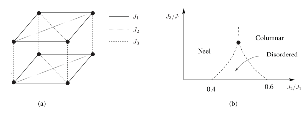
Our model is a 3-dimensional spin-1/2 antiferromagnet, on a tetragonal lattice, as shown in Figure 1(a). Frustrating interactions occur in the x-y plane but not in the third direction. All interactions are antiferromagnetic.
The Hamiltonian, in standard notation, is
| (1) |
where the summations are over the three classes of coupling respectively.
In the following section, section II, we present our zero temperature calculations and results, for the ground state energy and sublattice magnetization (order parameter), for both the Néel and columnar phases. Our results support a phase diagram of the form shown in Figure 1(b), and we estimate the location of the triple point at and Our series results are compared with the results of linear spin-wave theory. In section III we use series methods to compute the 1-magnon dispersion curves, in both ordered phases, and again compare our results with the spin-wave predictions. The spin-wave theory follows standard lines and, for completeness, is outlined in the appendix. In section IV we present our conclusions and discussion.
II Ground State Bulk Properties
The series expansion method is based on perturbative calculations for a sequence of finite connected clusters, which are then combined to obtain a series for the bulk system. In practice it is possible to treat of order different clusters and to obtain series of order 10-20 terms, depending on the model. The Hamiltonian is written in the standard form where has a simple known ground state. In the present work we use an Ising expansion in which consists of the diagonal terms and the quantum fluctuations are included in the perturbation . Series are obtained in powers of , and extrapolated to via standard Padé or differential approximant methods. The interested reader is referred to the book ohweihong for more detail.


II.1 Néel Phase
It is well known that the unfrustrated square lattice () has reduced Néel order in the ground state. This is a 2-sublattice structure with spins pointing in opposite directions on the two sublattices. For technical reasons it is useful to perform a spin rotation on the B sublattice, making the unperturbed ground state ferromagnetic. The Hamiltonian, for a lattice of sites is then written as
| (2) |
with
| (3) |
| (4) |
We have added and subtracted constant terms to make the unperturbed energy zero.
We have obtained series for the ground state energy and the magnetization to order . The rapid proliferation of clusters with 3 bond types (there are 320274 with 9 or fewer sites) limits the length of the series obtainable. The data are far too extensive to present, but can be provided on request. The values of and can then be estimated, with some uncertainty, for any values of and . It is convenient to set to set the energy scale. A display of the results is deferred to the third subsection, where they are presented together with the results for the columnar phase.
II.2 Columnar Phase
In the columnar phase the spins on alternating columns in a particular x-y plane will point in opposite directions. This satisfies all of the strong bonds but leaves half of the bonds frustrated. In adjacent planes these are shifted by one lattice spacing, leaving all of the bonds satisfied. This structure has an additional 2-fold degeneracy as columns can equally well be ‘rows’. Again it is convenient to carry out a spin rotation on ‘down’ sites, yielding
| (5) |
with
| (6) |
| (7) |
Here the notations and refer to nearest neighbor bonds in the and direction in a plane, respectively. We have calculated the expansion to order inclusive, involving a total of 114650 distinct clusters with 4 types of bond.


II.3 Results
Series were computed and analysed for the cases and a range of values of in both the Néel and columnar phases. We set throughout.
Figure 2 shows estimates of the ground state energy per site versus for two cases, (Fig.2a) and (Fig.2b).The energy is evaluated by forming Padé approximants to the series and evaluating these at . Error bars, where shown, represent confidence limits, based on the degree of consistency between high-order approximants.
As is apparent, the behaviour of the energy estimates is quite different in the two cases. For , i.e the square lattice model, the energy estimates in the intermediate range become erratic and the two curves, from the Néel and columnar series respectively, do not appear to join. However, for , the estimates are quite precise and the two curves cross near . The clear difference in slope of the two branches at the crossing point indicates a direct first-order transition between the two phases.
To analyse the magnetization series we first performed a Huse transformation huse1988 to a new variable to remove the square-root singularity at , expected from spin-wave theory. This procedure has been used in earlier work on the 2D antiferromagnet huse1988 ; zheng1991 . Padé approximants to the new series were then evaluated at .
The results are shown in Figure 3 and again display a striking difference between the two cases and . For we see clear evidence of an intermediate non-magnetic phase, with Néel and columnar magnetizations vanishing near and respectively. The error bars are large near the transition points and it is not possible to say whether the transitions are first- or second-order. It is generally believed that the columnar-disordered transition is first-order while the Néel-disordered transition appears second-order but may, in fact, be weakly first-order sirker . On the other hand, for (Fig.3b) it is clear that both magnetizations remain finite throughout their phase. This is consistent with a direct first-order transition.
Proceeding in this way with other values of , we construct a phase diagram as shown in Figure 4, which confirms the schematic phase diagram in Figure 1b. As is apparent, the disordered phase narrows as the interplane coupling is increased, and vanishes at the estimated point . This value of is a little lower than found previously schmalfuss .

III Excitations
It is also of interest to investigate the spectrum of single-magnon excitations in the ordered phases and to see how these change on increasing the interlayer coupling . Standard series methods exist for calculating the excitation energy throughout the Brillouin zone ohweihong , and we utilize these in the following.


III.1 Néel Phase
Series were obtained to order , based on 255196 distinct clusters of up to 8 sites. In Fig. 5 we show dispersion curves for two values of the frustrating interaction for , along various symmetry lines in the Brillouin zone, as shown. For comparison we also show the results of linear spin-wave theory.
Several features are worth noting:
-
(1)
A very pronounced dip develops at wavevector (and, by symmetry, also at ) with increasing . Linear spin-wave theory has the gap vanishing at (see Appendix).
-
(2)
There is a distinct ‘shoulder’ at , which is not seen in linear spin-wave theory. Indeed, along the whole line the energy depends only weakly on .
-
(3)
Linear spin-wave theory reproduces the overall dispersion curves reasonably well, but systematically underestimates the excitation energies.
We note also that the series become very irregular near the Goldstone point , and the Padé approximants do not accurately show the vanishing of the gap at this point. This has been noted in previous work singh1993 , and an indirect way found to overcome this problem, which also allows calculation of the spin-wave velocity. However, we do not address this further in the present work.
III.2 Columnar Phase
Series were obtained to order , based on 490487 distinct ckusters with up to 8 sites, and 4 possible bond types. In Figure 6 we show dispersion curves for and along various symmetry lines in the Brillouin zone. The predictions of linear spin-wave theory are shown as dashed lines.
The most notable feature is the depressed excitation energy along the line to . The dispersion curve in this region flattens as decreases from 1.0 to 0.6, in both cases (a) and (b). According to linear spin-wave theory this whole branch becomes soft at , the classical transition point. Again linear spin-wave theory tends to underestimate the excitation energy, but not as badly as for the Néel phase. The same difficulty with the Goldstone point , discussed above for the Néel phase, occurs here.
III.3 The Energy Gap at
As the phase transition is approached, from either the Néel or columnar side, we expect increasing quantum fluctuations at wavevector , which should be manifest through a decreasing energy gap at this point. As mentioned above, linear spin-wave theory predicts a vanishing excitation energy at this point at the classical transition point . Hence the variation of the gap is of some interest, and our results are shown in Figure 7, as a function of , for two values of the coupling ratio .
In the case (Fig. 7b) the gaps remain of substantial size right up to the direct first-order transition, and the gaps appear to be of roughly equal magnitude in both phases at the transition. This is a further sign that the transition between the two ordered phases is first order at this value of .
Figure 7a shows the energy gap at . Note that whereas linear spin wave theory has the gap vanishing at all couplings in the columnar phase, it is in fact finite at larger , as given by a modified spin-wave theory and earlier series results singh2 . Note also that the energy gaps in both phases extrapolate to zero before reaching the classical transition point , providing further evidence of a disordered intermediate phase when . Taken at face value, the results indicate that the gap remains finite at the estimated transition points and , which would indicate first order transitions. Naive extrapolations are not entirely reliable near a critical point, however, and a more precise check of this point would be of interest. A Dlog Padé analysis of the series in gives no consistent estimates of the critical point in this case.
IV conclusions
We have used series expansion methods to study a system of stacked layers with antiferromagnetic coupling between the layers. This model is applicable to the layered materials Li2VOSiO4 and Li2VOGeO4, as well as being of intrinsic theoretical interest. In agreement with earlier work of Schmalfuss et el. schmalfuss , we find that the disordered region of the phase diagram becomes narrower as is increased, and vanishes completely at a triple point, beyond which there is a direct first-order transition between the Néel and columnar phases. We estimate the location of the triple-point as , the value being somewhat lower than in ref. schmalfuss .
As well as mapping out the phase ground state phase diagram, we have computed magnon dispersion curves along symmetry lines in the Brillouin zone, in both the Néel and columnar phases, for various parameter values. This would allow a more critical evaluation of the validity of the model for the materials mentioned above, when experimental inelastic neutron scattering results for magnon energies become available.
After this work had been completed we became aware of two other recent studies of this model. Nunes et al. nunes , using an effective field theory approach, concluded that the triple point (they refer to this as a critical end-point, assuming the Néel to disordered transition is second order) lies at , values much higher than obtained in the present work and in other work schmalfuss ; Holt . Majumdar majumdarnew has carried out a spin-wave calculation to second order () and concludes that the intermediate phase remains present even at , which seems surprising in view of the other work referred to above.
Finally we mention another recent study majumdar of a different generalization of the 2-dimensional model, in which the frustrating interactions are included in all spatial directions. That model appears also to have an interesting phase diagram, and could be studied by series methods.
V Acknowledgements
We are grateful for the computing resources provided by the Australian Partnership for Advanced Computing (APAC) National Facility.
Appendix A Linear Spin-Wave Theory
In the Appendix we present the results of linear spin-wave theory (LSWT) for the model, for both the Néel and columnar phases. The results have been used in the main text to compare with the more accurate series results.
The basic procedures of LSWT are well known so we will not include all details.
A.1 Néel Phase
There are two equivalent sublattices A, B and two sets of bosons describing spin deviations from the classical Néel state. After Fourier transformation the Hamiltonian is, to quadratic order
| (8) | |||||
with
| (9) |
This is then diagonalized by a standard Bogoliubov transformation, yielding
| (10) |
with
| (11) |
The ground state energy is
| (12) |
and the sublattice magnetization is
| (13) |
We note that for small
| (14) |
so there is a linear Goldstone mode at , provided . The phase becomes unstable for .
Another special case occurs at . Let be small, then
| (15) | |||||
Hence the gap at vanishes at , regardless of , corresponding to a phase transition.
A.2 Columnar Phase
There are again two sublattices, with the A and B sites forming successive columns. The Fourier transformed Hamiltonian is now
| (16) | |||||
A Bogoliubov transformation then yields
| (17) |
with
| (18) |
and
| (19) | |||||
The sublattice magnetization is again given by the formula (13).
For small
| (20) | |||||
which shows that again there is a Goldstone mode at , which is stable for , but becomes unstable at .
Another special case is , when
| (21) |
Hence vanishes along this line at , corresponding again to the transition point.
References
- (1) P. Chandra and B. Doucot, Phys. Rev. B 38, 9335 (1988).
- (2) E. Dagotto and A. Moreo, Phys. Rev. Lett. 63, 2148 (1989).
- (3) H.J. Schulz and T.A.L. Ziman, Europhys. Lett. 18, 355 (1992); H.J. Schulz, T.A.L. Ziman and D. Poilblanc, J. Phys. I6, 675 (1996).
- (4) J. Richter, Phys. Rev. B47, 5794 (1993); J. Richter, N.B. Ivanov and K. Retzlaff, Europhys. Lett. 25, 545 (1994).
- (5) J. Oitmaa and Zheng Weihong, Phys. Rev. B 54, 3022 (1996).
- (6) R.F. Bishop, D.J.J. Farnell and J.B. Parkinson, Phys. Rev. B58, 6394 (1998).
- (7) R.R.P. Singh, Zheng Weihong, C.J. Hamer and J. Oitmaa, Phys. Rev. B60, 7278 (1999).
- (8) L. Capriotti and S. Sorella, Phys. Rev. Lett. 84, 3173 (2000).
- (9) L. Siurakshina, D. Ihle and R. Hayn, Phys. Rev. B64, 104406 (2001).
- (10) O. P. Sushkov, J. Oitmaa and Z. Weihong, Phys. Rev. B 63, 104420 (2001).
- (11) L. Capriotti, F. Becca, A. Parola and S. Sorella, Phys. Rev. Lett. 87, 097201 (2001).
- (12) L. Capriotti, F. Becca, A., Parola, A., and S. Sorella, Phys. Rev. B 67, 212402 (2003).
- (13) R.R.P. Singh, Weihong Zheng, J. Oitmaa, O.P. Sushkov and C.J. Hamer, Phys. Rev. Lett. 91, 017201 (2003).
- (14) T. Roscilde, A. Feiguin, A.L. Chernyshev, S. Liu and S. Haas, Phys. Rev. Lett. 93, 017203 (2004).
- (15) J. Sirker, Z. Weihong, O. P. Sushkov and J. Oitmaa, Phys. Rev. B 73, 184420 (2006).
- (16) D. Schmalfuss, R. Darradi, J. Richter, J. Schulenberg and D. Ihle, Phys. Rev. Lett. 97, 157201 (2006).
- (17) J. Oitmaa, C. J. Hamer and Z. Weihong, Series Expansion Methods for Strongly Interacting Lattice Models, Cambridge, (2006)
- (18) H. Rosner, R. R. P. Singh, W. H. Zheng, J. Oitmaa, S.-L. Drechsler and W. E. Pickett, Phys. Rev. Lett. 88, 186405 (2002); H. Rosner, R. R. P. Singh, W. H. Zheng, J. Oitmaa, and W. E. Pickett, Phys. Rev. B 67, 014416 (2003).
- (19) G. S. Uhrig, M. Holt, J. Oitmaa, O. P. Sushkov, and R. R. P. Singh, Phys. Rev. B 79, 092416 (2009).
- (20) M. Holt, O.P. Sushkov, D. Stanek and G.S. Uhrig, preprint arXiv:1010.5551v1 (2010)
- (21) D. A. Huse, Phys. Rev. B 37, 2380 (1988).
- (22) Zheng Weihong, J. Oitmaa and C.J. Hamer, Phys. Rev. B 43, 8321 (1991).
- (23) R.R.P. Singh, Phys. Rev. B47, 12337 (1993); R.R.P. Singh and M.P. Gelfand, ibid. 52, R15695 (1995).
- (24) W. A. Nunes, J. Ricardo de Sousa, J. Roberto Viana and J. Richter, J. Phys. Cond. Mat. 22, 146004 (2010).
- (25) K. Majumdar, J. Phys. Cond. Mat. 23, 046001 (2011).
- (26) K. Majumdar and T. Datta, J. Stat. Phys. 139, 714 (2010).