The thermodynamic properties of Davydov-Scott’s protein model in thermal bath

Abstract

The thermodynamic properties of Davydov-Scott monomer contacting with thermal bath is investigated using Lindblad open quantum system formalism. The Lindblad equation is investigated through path integral method. It is found that the environmental effects contribute destructively to the specific heat, and large interaction between amide-I and amide-site is not preferred for a stable Davydov-Scott monomer.

1 Introduction

Does the Davydov-Scott’s soliton exist at biological temperature ? The question has attracted more interest in the last decades [1, 2, 3, 4]. Earlier studies using finite temperature molecular dynamics showed that the Davydov soliton lifetime is only few picoseconds which is too short at the biological temperature. The reason is the random thermal prevents Davydov self-trapping from occurring as, for example as discussed in [5] which showed that the two-quantum state might be more stable than the one-quantum state. Furthermore, using the standard Davydov model, some numerical calculations also indicated that soliton is stable at 310K. On the other hand, the analytic calculation based on trial function or perturbation methods obtained that soliton is stable at 300K [6, 7].

The above-mentioned calculations were performed using the equilibrium quantum system at finite temperature [8]. The finite temperature means that the quantum system is in contact with environment such as thermal bath. The interaction of a system with its environment is given by the dissipation effect in quantum system. However, the dissipation effect leads to a serious problem for quantization procedure. The most appropriate theory to resolve this problem is the Quantum State Diffusion (QSD) based on Lindblad formulation [9]. The first application of QSD to the protein model has been done by Cuevas et.al.[4]. Their calculation on Davydov-Scott monomer showed that at room temperature the semi classical approach might be a good approximation compared to the corresponding full quantum system. However the study was focused on the dynamical aspect of the system, i.e. the solution of Heisenberg’s picture and its wave function based on the QSD equation. Recent studies of the anharmonic effect for the monomer has also been done by us using path integral and the thermodynamic function [10]. The advantage of calculating thermodynamic function is also relevant in another approaches such as the models describing the phenomena in term of elementary matter interactions using lagrangian [11]. It was argued that the thermodynamic properties should be easier to observe than another ones based on the wave function. Therefore, it is important to study such system from statistical mechanics point of view.

The paper studies the thermodynamic properties of Davydov-Scott monomer including the thermal bath. The effect of thermal bath is investigated using the Lindblad open quantum system formalism through path integral method. The temperature dependencies of the system are obtained for the normalized specific heat. It is shown that the specific heat is sensitive to the size of coupling constant between amide-I and amide-site.

The paper is organized as follows. In Sec. 2 the Davydov Hamiltonian for a one-dimensional molecular monomer is described and the thermal bath effect is studied in Lindblad equation. In Sec. 3 the thermodynamic properties are investigated using path integral method. The paper is ended by a short summary.

2 Lindblad open quantum system formulation

We use Davydov-Scott’s model of the alpha-helix protein. The Davydov-Scott monomer is a coupled of the amide-I oscillator that expressed by the coordinate ($x$) and momentum ($p$) operators, and the amide-site is expressed by the displacement and momentum operators, $Q$ and $P$, respectively. Hamiltonian in the model has the form [10],

$$H=\frac{p^{2}}{2m}+\frac{1}{2}m\omega^{2}x^{2}+\frac{P^{2}}{2M}+\frac{1}{2}\kappa Q^{2}+\chi xQ\;,$$ (1)

where $\omega$ is the intrinsic frequency of amide-I oscillation, $\chi$ is the coupling constant between two oscillators, $m$ ($M$) is the amide-I (amide-site) mass and $\delta$ is the anharmonic coefficient. Throughout the paper we also use the notations $\chi^{\prime}=\chi\sqrt{{2M\Omega}/\hbar}$ and $\Omega=\sqrt{\kappa/M}$. The Hamiltonian describes the Davydov-Scott’s monomer as a coupled harmonic oscillator.

If the environmental or dissipation effect can not be ignored, the physical system is not reversible. In another words, the irreversibility implies the dissipation effect in a quantum system under consideration. One of the basic tools to introduce dissipation in quantum mechanics is the dynamical semi groups, and called as the Lindblad open quantum system formalism. In particular, the quantum system whose the wave function equation can be obtained from the Lindblad equation is called as QSD [9].

According to Lindblad formalism, the usual von Neumann-Liouville equation is replaced by Lindblad equation or master equation in the form of,

$$\frac{\partial\rho}{\partial t}=-\frac{i}{\hbar}[H,\rho]+\sum_{j}(L_{j}\rho L^{\dagger}_{j}-\frac{1}{2}L^{\dagger}_{j}L_{j}\rho-\frac{1}{2}\rho L^{\dagger}_{j}L_{j})\;.\$$ (2)

$\rho$ is the density function and $L_{j}$ denotes the Lindblad operator which may neither Hermitian nor unique. In this formalism, the operator $H$ describes internal dynamics, while $L$ represents the environmental effects in the system.

Throughout the paper, let us assume that the environmental strength of the amide-site is stronger than the amide-I excitation. Since $L$ must be the first order in $Q$ and $P$, we choose the Lindblad operators as follow,

$$L_{1} = \sqrt{\gamma(1+\nu)}\left(\sqrt{\frac{M\Omega}{2\hbar}}Q+i\sqrt{\frac{1}{2M\hbar\Omega}}P+\frac{\chi^{\prime}}{\hbar\Omega}\sqrt{\frac{m\omega}{2\hbar}}x\right)\;,$$ (3)

$$L_{2} = \sqrt{\gamma\nu}\left(\sqrt{\frac{M\Omega}{2\hbar}}Q-i\sqrt{\frac{1}{2M\hbar\Omega}}P+\frac{\chi^{\prime}}{\hbar\Omega}\sqrt{\frac{m\omega}{2\hbar}}x\right)\;.\$$ (4)

$\gamma$ is a damping parameter and $\nu=\left(\mathrm{e}^{{\hbar\Omega}/{k_{B}T}}-1\right)^{-1}$ is Bose-Einstein distribution function with the Boltzman coefficient $k_{B}$.

The master equation in Eq.(2) is calculated using Feynman path integral. Assuming the diffusion term is dominant over the frictional damping rate ($[Q,[Q,\rho]]\gg[Q,[P,\rho]]$), Eq. (2) is rewritten in a differential representation,

$$\frac{\partial\rho}{\partial t} = \frac{i\hbar}{2m}\left(\frac{\partial^{2}}{\partial x^{2}}-\frac{\partial^{2}}{\partial x^{\prime 2}}\right)\rho-\left(\frac{im\omega^{2}}{2\hbar}+\frac{\delta_{3}}{2\hbar^{2}}\right)\left(x^{2}-x^{\prime 2}\right)\rho$$ (5)

$$+\left(\frac{i\hbar}{2M}+\frac{\delta_{1}}{2\hbar}\right)\left(\frac{\partial^{2}}{\partial Q^{2}}-\frac{\partial^{2}}{\partial Q^{\prime 2}}\right)\rho-\left(\frac{iM\Omega^{2}}{2\hbar}+\frac{\delta_{2}}{2\hbar}\right)(Q^{2}-Q^{{}^{\prime}2})\rho$$

$$-i\left(\frac{\chi}{\hbar}+\frac{\delta_{4}}{2\hbar}\right)\left(xQ-x^{\prime}Q^{\prime}\right)\rho\;.$$

Here, the Lindblad’s coefficients are $\delta_{1}=\gamma(1+2\nu)/(2M\Omega)$, $\delta_{2}={\gamma(1+2\nu)M\Omega}/2$, $\delta_{3}=\gamma(1+2\nu){(\chi^{2}m\omega)}/(\hbar\Omega)^{2}$ and $\delta_{4}=\sqrt{m\omega M\Omega}\chi^{\prime}/{(\hbar\Omega)}$. The propagator of Eq. (5) is given by,

$$K(x,x^{\prime};Q,Q^{\prime}) = \int\int{\cal D}[x]{\cal D}[Q]\mathrm{exp}\left[\frac{i}{\hbar}\int\mathrm{d}t\left(\frac{1}{2}m\dot{x}^{2}-\frac{1}{2}m\tilde{\omega}^{2}x^{2}\right.\right.$$ (6)

$$+\left.\left.\frac{1}{2}\bar{M}\dot{Q}^{2}+\frac{1}{2}\bar{M}\tilde{\Omega}^{2}Q^{2}-\tilde{\chi}^{\prime}xQ\right)\right]\;,$$

where $\tilde{\omega}^{2}=\omega^{2}+{i\delta_{3}}/{(m\hbar)}$, $\tilde{\Omega}^{2}=\Omega^{2}+{i\delta_{2}}/{(M\hbar)}$, $\bar{M}=M+{i\hbar^{2}}/{\delta_{1}}$ and $\tilde{\chi}=\chi+\delta_{4}/2$. Making use of the Gaussian approximation, only the classical path of amide-site ($\bar{Q}$) contributes to the interaction term [12, 13]. It yields,

$$K(x,x^{\prime};Q,Q^{\prime}) = K_{x}K_{Q}$$ (7)

$$= \int{\cal D}[x]\mathrm{exp}\left[-\frac{i}{\hbar}\int\mathrm{d}t\left(\frac{1}{2}m\dot{x}^{2}-\frac{1}{2}\tilde{\omega}^{2}x^{2}-\tilde{\chi}x\bar{Q}\right)\right]$$

$$\times\int{\cal D}[Q]\mathrm{exp}\left[-\frac{i}{\hbar}\int\mathrm{d}t\left(\frac{1}{2}\bar{M}\dot{Q}^{2}-\frac{1}{2}\bar{M}\tilde{\Omega}^{2}Q^{2}\right)\right]\;.$$

The propagator $K_{Q}$ is just a harmonic oscillator, and the solution is well known [13, 14],

$$K(Q,t;Q^{\prime},0) = \mathrm{exp}\left[-i\frac{\pi}{2}\left(\frac{1}{2}+\left|\frac{\tilde{\Omega}t}{\pi}\right|\right)\right]\sqrt{\frac{\bar{M}\tilde{\Omega}}{2\pi\hbar|\sin(\tilde{\Omega}t)|}}$$ (8)

$$\times\mathrm{exp}\left\{\frac{i\bar{M}\tilde{\Omega}}{2\hbar|\sin(\tilde{\Omega}t)|}\left[(Q^{\prime 2}+Q^{2})\cos(\tilde{\Omega}t)-2QQ^{\prime}\right]\right\}\;.$$

where $\|x\|$ denotes the largest integer smaller than $x$.

The propagator of $K_{x}$ is a driven harmonic oscillator and the solution is also known [13, 14]. The driven function $\bar{Q}$ is the classical solution of equation of motion (EOM) of $Q$, that is a harmonic oscillator. Taking the solution $\bar{Q}=\bar{Q}_{0}\sin(\tilde{\Omega}t)$ and substituting it into the path integral solution of a driven harmonic oscillator, then the propagator becomes [13, 14],

$$K(x,t;x^{\prime},0)=\mathrm{exp}\left[-i\frac{\pi}{2}\left(\frac{1}{2}+\left|\frac{\tilde{\omega}t}{\pi}\right|\right)\right]\sqrt{\frac{m\tilde{\omega}}{2\pi\hbar|\sin(\tilde{\omega}t)|}}\mathrm{e}^{\frac{i}{\hbar}S_{\mathrm{cl}}}\;,$$ (9)

where $S_{\mathrm{cl}}$ is given by,

$$S_{\mathrm{cl}} = \frac{m\tilde{\omega}}{2\sin(\tilde{\omega}t)}\left[(x^{2}+x^{\prime 2})\cos(\tilde{\omega}t)-2xx^{\prime}\right]$$

$$+\frac{\tilde{\chi}\bar{Q}_{0}x^{\prime}}{(\tilde{\Omega}^{2}-\tilde{\omega}^{2})\sin(\tilde{\omega}t)}\left[\tilde{\omega}\cos(\tilde{\omega}t)\sin(\tilde{\Omega}t)-\tilde{\Omega}\sin(\tilde{\omega}t)\cos(\tilde{\Omega}t)\right]$$

$$+\frac{\tilde{\chi}\bar{Q}_{0}x}{(\tilde{\Omega}^{2}-\tilde{\omega}^{2})\sin(\tilde{\omega}t)}\left[\tilde{\Omega}\sin(\tilde{\omega}t)-\tilde{\omega}\sin(\tilde{\Omega}t)\right]$$

$$+\frac{\tilde{\chi}^{2}\bar{Q}_{0}^{2}}{m\tilde{\omega}(\tilde{\Omega}^{2}-\tilde{\omega}^{2})\sin(\tilde{\omega}t)}\left[A\cos(\tilde{\omega}t)\sin^{2}(\tilde{\Omega}t)+B\sin(\tilde{\omega}t)\sin(2\tilde{\Omega}t)-\frac{\tilde{\omega}}{4}t\right]\;.$$

with $A=\tilde{\omega}(\tilde{\omega}\tilde{\Omega}+1)/(4(\tilde{\Omega}^{2}-\tilde{\omega}^{2}))$ and $B=-\tilde{\omega}(\tilde{\Omega}^{2}+\tilde{\omega}^{2})/(8\tilde{\Omega}(\tilde{\Omega}^{2}-\tilde{\omega}^{2}))$.

Combining Eqs. (9) and (2), the propagator $K(x,x^{\prime};Q,Q^{\prime};t,t^{\prime})$ becomes,

$$K(Q,x,t;Q^{\prime},x^{\prime},0) = \mathrm{exp}\left[-i\pi\left(\frac{1}{2}+\frac{1}{2}\left|\frac{(\tilde{\Omega}+\tilde{\omega})t}{\pi}\right|\right)\right]$$

$$\times\sqrt{\frac{\bar{M}\tilde{\Omega}}{2\pi\hbar|\sin(\tilde{\Omega}t)|}}\sqrt{\frac{m\tilde{\omega}}{2\pi\hbar|\sin(\tilde{\omega}t)|}}$$

$$\times\mathrm{exp}\left\{\frac{\bar{iM}\tilde{\Omega}}{2\hbar|\sin(\tilde{\Omega}t)|}\left[(Q^{\prime 2}+Q^{2})\cos(\tilde{\Omega}t)-2QQ^{\prime}\right]+\frac{i}{\hbar}S_{\mathrm{cl}}\right\}\;.$$

3 Thermodynamic properties

The discussion of a system interacting with heat bath is characterized by the temperature $T$. The state of those systems is therefore given by an equilibrium density matrix which can be obtained by performing a transformation $t\rightarrow\tau=-i\hbar\beta$ in the propagator with $\beta=1/(k_{B}T)$ [13, 14]. The density matrix is actually the propagator with $\rho(x,x,Q,Q,\tau,0)=K(Q,x;Q,x,\tau,0)$. Substituting $t\rightarrow\tau=-i\hbar\beta$ into Eq. (2), one obtains,

$$\rho_{\beta}(x,Q) = \mathrm{exp}\left[-i\pi\left(\frac{1}{2}-\frac{i}{2}\left|\frac{(\tilde{\Omega}+\tilde{\omega})\hbar\beta}{\pi}\right|\right)\right]$$ (12)

$$\times\sqrt{\frac{\bar{M}\tilde{\Omega}}{2\pi\hbar\sinh(\tilde{\Omega}\hbar\beta)}}\sqrt{\frac{m\tilde{\omega}}{2\pi\hbar\sinh(\tilde{\omega}\hbar\beta)}}$$

$$\times\mathrm{exp}\left\{-\frac{\bar{M}\tilde{\Omega}}{\hbar}\tanh(\frac{1}{2}\Omega\hbar\beta)Q^{2}-\frac{m\tilde{\omega}}{\hbar}\tanh(\frac{1}{2}\omega\hbar\beta)x^{2}\right.$$

$$+\left.\frac{2\tilde{\chi}\bar{Q}_{0}}{\hbar(\tilde{\Omega}^{2}-\tilde{\omega}^{2})}\left[\tilde{\Omega}\sinh^{2}(\frac{1}{2}\tilde{\Omega}\hbar\beta)-\tilde{\omega}\sinh(\tilde{\Omega}\hbar\beta)\sinh(\frac{1}{2}\tilde{\omega}\hbar\beta)\right]x\right.$$

$$+\left.\frac{\tilde{\chi}^{2}\bar{Q}_{0}^{2}}{m\tilde{\omega}\hbar^{2}(\tilde{\Omega}^{2}-\tilde{\omega}^{2})}\left[A\Omega\sinh^{2}(\tilde{\Omega}\hbar\beta)\coth(\tilde{\omega}\hbar\beta)+B\sinh(2\tilde{\Omega}\hbar\beta)\right.\right.$$

$$-\left.\left.\frac{\tilde{\omega}\hbar\beta}{4\sinh(\tilde{\omega}\hbar\beta)}\right]\right\}\;.$$

Having the density matrix at hand, in the statistical mechanics one can consider partition function [12],

$$Z(\beta)=\mathrm{e}^{-\beta F}=\int dx\int dQ\,\rho_{\beta}(x,Q)\;.$$ (13)

Substituting Eq. (12) into Eq. (13) and using the hyperbolic manipulation yield,

$$Z(\beta) = \frac{1}{2\sinh(\frac{1}{2}\tilde{\Omega}\hbar\beta)}\frac{1}{2\sinh(\frac{1}{2}\tilde{\omega}\hbar\beta)}\,\mathrm{exp}\left[-\frac{i\pi}{2}\left(1-\left|\frac{\tilde{\Omega}\hbar\beta}{\pi}\right|+\left|\frac{\tilde{\omega}\hbar\beta}{\pi}\right|\right)\right]$$

$$\times\mathrm{exp}\left[\frac{\tilde{\chi}^{2}\bar{Q}_{0}^{2}\left\{\tilde{\Omega}\sinh^{2}(\frac{1}{2}\tilde{\Omega}\hbar\beta)-\tilde{\omega}\sinh(\tilde{\Omega}\hbar\beta)\sinh(\frac{1}{2}\tilde{\omega}\hbar\beta)\right\}^{2}}{\hbar\bar{M}\tilde{\Omega}(\tilde{\Omega}^{2}-\tilde{\omega}^{2})\tanh(\frac{1}{2}\tilde{\omega\hbar\beta})}\right.$$

$$+\left.\frac{\tilde{\chi}^{2}\bar{Q}_{0}^{2}\left\{A\Omega\sinh^{2}(\tilde{\Omega}\hbar\beta)\cosh(\tilde{\omega}\hbar\beta)+B\sinh(2\tilde{\Omega}\hbar\beta)\sinh(\tilde{\omega}\hbar\beta)-\frac{1}{4}\tilde{\omega}\hbar\beta\right\}}{m\tilde{\omega}\hbar^{2}(\tilde{\Omega}^{2}-\tilde{\omega}^{2})\sinh(\tilde{\omega}\hbar\beta)}\right]\;,$$

by borrowing the Gaussian integral, $\int dx\,\mathrm{exp}(-ax^{2}+bx+c)=\sqrt{\pi/a}\,\mathrm{exp}[{b^{2}}/{(4a)}+c]$.

For an open quantum system, such as the Davydov-Scott monomer, the changes of the surrounding environment entropy must be taken into account. The effect is conveniently incorporated by the specific heat which is also experimentally measurable. It describes the quantities of heat that must be added to a system in order to increase its temperature, and defined as [12],

$$C=k_{B}\beta^{2}\frac{\partial^{2}\ln Z}{\partial\beta^{2}}\;.\$$ (15)

Bringing Eq. (3), one gets,

$$\frac{C}{k_{B}}=\frac{I^{2}}{\sinh^{2}I}+\frac{w^{2}}{\sinh^{2}(w)}+\tilde{\chi}^{2}\Lambda(\beta)\;,$$ (16)

where $I={\tilde{\Omega}\hbar\beta}/2$, $w={\tilde{\omega}\hbar\beta}/2$ and,

$$\Lambda(\beta) = \frac{\bar{Q}_{0}^{2}\beta^{2}}{2\hbar}\frac{\partial^{2}}{\partial\beta^{2}}\left\{\frac{\left[\tilde{\Omega}\sinh^{2}I-\tilde{\omega}\sinh(2I)\sinh w\right]^{2}}{\bar{M}\tilde{\Omega}(\tilde{\Omega}^{2}-\tilde{\omega}^{2})\tanh w}\right.$$ (17)

$$+\left.\frac{A\Omega\sinh^{2}(2I)\cosh(2w)+B\sinh(4I)\sinh(2w)-\frac{1}{2}w}{m\tilde{\omega}\hbar(\tilde{\Omega}^{2}-\tilde{\omega}^{2})\sinh(2w)}\right\}\;.$$

For small coupling case we have approximately $\sinh(x)\sim x$, $\cosh(x)\sim 1$ and $\tanh(x)\sim x$ to yield,

$$\Lambda(\beta)=\frac{\bar{Q}_{0}^{2}}{2\hbar(\tilde{\Omega}^{2}-\tilde{\omega}^{2})}\left(\frac{3}{4}\tilde{\Omega}^{3}-\frac{3}{2}\tilde{\Omega}^{2}\tilde{\omega}^{2}-3\tilde{\omega}^{4}\tilde{\Omega}\right)\beta^{3}\;.\$$ (18)

The specific heat in Eq. (16) can be read as,

$$C=C_{\mathrm{amide-site}}+C_{\mathrm{amide-I}}+C_{\mathrm{mixing}}\;.$$ (19)

If there is no coupling between amide-site and amide-I, i.e. $\tilde{\chi}=0$, this is just the total specific heat of two independent harmonic oscillators.

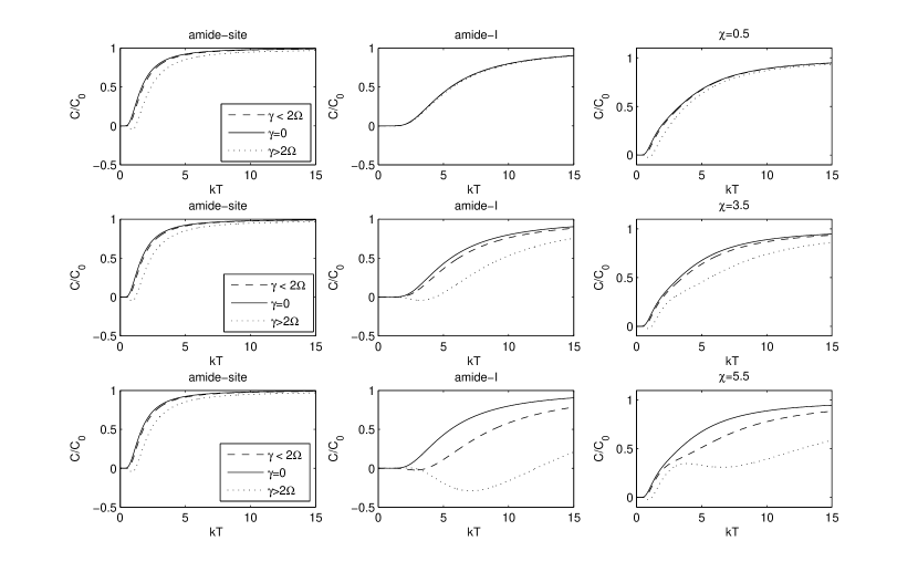
Figure 1: The temperature dependence of normalized specific heat for the first (left), second (middle) and total (right) terms in Eq. (19) for various values of $\gamma$.

The result is depicted in Fig. 1 for three cases corresponding to the values of $\gamma$, that is $\gamma=0$, $\gamma<\Omega$ and $\gamma>\Omega$. The case of non-zero but small $\gamma$ has similar behavior as non-damping case. All of them coincide each other at low temperature and tend to be asymptotically constant at high temperature. On the other hand, large $\gamma$ reduces the specific heat for the whole region of temperature. This means the environtmental effect contributes destructively to the specific heat, and the system requires less energy to increase the temperature to reach the equilibrium.

The application of the present model to the $\alpha-$helix protein requires proper knowledge on the coupling constant between amide-I and amide-site [3]. There are some attempts to determine its allowed range through several methods like the Ab initio calculation and also the extraction from the experimental data as well. The value is found to be within 7 pN and 62 pN [3]. Considering the amide-site mass $5.7\times 10^{-25}kg$ and the string constant $\kappa=58.5$ Nm^-1, one immediately obtains the coupling constant $\chi^{\prime}=1.7,11.6,18.2$ corresponding to $\chi=0.5,2.5,5.5$ pN. Note that most of previous works takes $\chi=62$ pN. However, those works do not take into account the thermal bath effect. On the other hand, including the thermal bath as done in the present paper enhance the contribution of amide-I and amide-site interaction.

The result is depicted in Fig. 1 showing the temperature dependencies of the normalized specific heat for various values of $\gamma$. The left, middle and right figures correspond to the contribution of the first term, the second term and the total in Eq. (19) respectively. From the figures one can conclude that the results are sensitive to the size of coupling constant $\chi$ at intermediate temperature. Especially, the amide-I is more affected than amide-site. The reason is because amide-I has higher frequency than amide-site. Moreover, amide-I is also suppressed significantly by thermal bath contribution which indicates the dependencies of system frequency on the effect of thermal bath as already pointed out by Ingold et.al.through Caldiora-Lenggets formalism [14].

It should be remarked that at low temperature region large environmental effect induces an anomaly, that is the specific heat is getting negative. This anomaly has also been observed by Ingold et.al.[15] for free harmonic oscillator using Caldiora-Lenggets formalism, and by us using full-quantum approach and the Lindblad formulation of master equation [10].

4 Summary

The interaction of Davydov-Scott monomer with thermal bath is investigated using the Lindblad open quantum system formalism. In contrast with previous work by Cuevas et.al.[4], the statistical partition function is calculated instead of solving the EOM itself.

Using path integral one can calculate the propagator of the Lindblad equation. Under an assumption that the diffusion term is dominant, we have shown that the environment contributions shift the kinetic, potential and interaction terms in the lagrangian. The mixing term is survive only if the frictional damping rate is taken into account.

In the open quantum system the damping coefficient $\gamma$ represents the relaxation time due to interaction with the environment. Non-zero $\gamma$ contributes destructively to the specific heat. The higher value of $\gamma$ corresponds to the shorter relaxation time, and it induces specific heat anomaly as pointed out in previous works [15, 10]. It is also found that large interaction between amide-I and amide-site is not preferred for a stable Davydov-Scott monomer.

References

• [1] L. Cruzeiro, J. Halding, P. L. Christiasen, O. Skovgard, A. C. Scott, Temperature effects on the davydov soliton, Physical Review A 37 (1988) 880–887.
• [2] L. Cruzeiro-Hansson, S. Takeno, Davydov model: The quantum, mixed quantum-classical, and full classical systems, Physical Review E 56 (1997) 894.
• [3] A. C. Scott, Davidov’s soliton, Physics Report 217 (1992) 167.
• [4] J. Cuevas, P. A. S. Silva, F. R. Romero, L. Cruzeiro, Dynamics of the davydov-scott monomer in a thermal bath: Comparison of the full quantum and semiclassical approaches, Physical Review E 76 (2007) 011907.
• [5] L. Cruzeiro-Hansson, Two reasons why the davydov soliton may be thermally stable after all, Physical Review Letters 73 (1994) 2927–2930.
• [6] J. P. Cottingham, J. W. Schweitzer, Calculation of the lifetime of a davydov soliton at finite temperature, Physical Review Letter 62 (1989) 1792–1795.
• [7] D. V. Kapor, M. J. Skrinjar, S. D. Stojanovic, Variational approach to davydov’s soliton theory for real phonons, Physical Review A 41 (1990) 5694–5701.
• [8] R. Luzzia, A. R. Vasconcellosa, J. Casas-Vazquezb, D. Jou, Characterization and measurement of a nonequilibrium temperature-like variable in irreversible thermodynamics, Physica A 234 (1997) 699.
• [9] I. Percival, Quantum State Diffusion, 2nd Edition, Cambridge Univ. Press, 1998.
• [10] A. Sulaiman, F. P. Zen, H. Alatas, L. T. Handoko, Anharmonic oscillation effect on the davydov-scott monomer in thermal bath, Physical Review E 81 (2010) 061907.
• [11] A. Sulaiman, L. T. Handoko, The effects of bio-fluid on the internal motion of dna, Journal of Computational and Theoretical Nanoscience 8 (2011) 124.
• [12] R. P. Feynmann, Statistical Mechanics, W. A. Benjamin Inc., 1965.
• [13] H. Kleinert, Path Integrals in Quantum Mechanics, Statistics, and Polymer Physics, and Financial Markets, World Scientific, 2009.
• [14] P. Hanggi, G.-L. Ingold, P. Talkner, Finite quantum dissipation: the challenge of obtaining specific heat, New Journal of Physics 10 (2008) 115008.
• [15] G.-L. Ingold, P. Hanggi, P. Talkner, Specific heat anomalies of open quantum systems, Physical Review E 79 (2009) 061105.