A search for new hot subdwarf stars by means of Virtual Observatory tools

Abstract

Context. Recent massive sky surveys in different bandwidths are providing new opportunities to modern astronomy. The Virtual Observatory (VO) provides the adequate framework to handle the huge amount of information available and filter out data according to specific requirements.

Aims. Hot subdwarf stars are faint, blue objects, and are the main contributors to the far-UV excess observed in elliptical galaxies. They offer an excellent laboratory to study close and wide binary systems, and to scrutinize their interiors through asteroseismology, as some of them undergo stellar oscillations. However, their origins are still uncertain, and increasing the number of detections is crucial to undertake statistical studies. In this work, we aim at defining a strategy to find new, uncatalogued hot subdwarfs.

Methods. Making use of VO tools we thoroughly search stellar catalogues to retrieve multi-colour photometry and astrometric information of a known sample of blue objects, including hot subdwarfs, white dwarfs, cataclysmic variables and main sequence OB stars. We define a procedure to discriminate among these spectral classes, particularly designed to obtain a hot subdwarf sample with a low contamination factor. In order to check the validity of the method, this procedure is then applied to two test sky regions: the Kepler FoV and to a test region of 300 deg² around ($\alpha$:225, $\delta$:5) deg.

Results. As a result of the procedure we obtained 38 hot subdwarf candidates, 23 of which had already a spectral classification. We have acquired spectroscopy for three other targets, and four additional ones have an available SDSS spectrum, which we used to determine their spectral type. A temperature estimate is provided for the candidates based on their spectral energy distribution, considering two-atmospheres fit for objects with clear infrared excess, as signature of the presence of a cool companion. Eventually, out of 30 candidates with spectral classification, 26 objects were confirmed to be hot subdwarfs, yielding a contamination factor of only 13%. The high rate of success demonstrates the validity of the proposed strategy to find new uncatalogued hot subdwarfs. An application of this method to the entire sky will be presented in a forthcoming work.

1 Introduction

Hot subdwarf stars (hot sds), objects with temperatures exceeding 19 000 K and $\log g\geq$ 5, are considered to be the field counterparts of the extended horizontal-brach (EHB) stars found in globular clusters. Such an evolutionary state implies a $\sim 0.5\leavevmode\nobreak\ M_{\odot}$ canonical mass, and a core He-burning structure with a very thin H-envelope (M_env $\leq$ 0.02$M_{\odot}$, Heber 1986). This structure prevents them from ascending the asymptotic giant branch (AGB) and, once the core helium is exhausted, they evolve towards hotter temperatures before reaching degeneracy and cooling as a normal white dwarf star (Dorman et al. 1993).

Whereas the role of hot subdwarfs as white dwarf progenitors is well understood, the circumstances that lead to the removal of all but a tiny fraction of the hydrogen envelope, at about the same time as the core has achieved the mass required for the He flash ($\approx 0.47\leavevmode\nobreak\ M_{\odot}$), are still a matter of debate. Two main scenarios have been proposed to explain the formation of these objects: i) enhancement of the mass loss efficiency near the red giant branch (RGB) tip (D’Cruz et al. 1996); ii) mass transfer through binary interaction (Mengel et al. 1976).

A large fraction of hot subdwarfs are observationally found in binary systems (Ulla & Thejll 1998; Maxted et al. 2001), supporting the mass transfer scenario. However, a non negligible percentage appear as single hot sds. From a single evolution point of view, it is unknown, though, what could cause an enhanced mass loss at the RGB. Binary population synthesis by Han et al. (2002, 2003) show that common envelope ejection (CEE), stable Roche lobe overflow and helium white dwarfs merging can produce hot sds in close or wide binaries, as well as single sds. These different paths produce distinct orbital period distributions and a variety of mass ranges for the hot sds and binary companions. A confrontation of theory and observations could be the key to clarify the hot sds evolutionary state and, moreover, help to fine-tune the processes related to the CEE. Some attempts have already been made in this direction (Morales-Rueda et al. 2003; Stroeer et al. 2007), however, the observed orbital period distribution is biased towards the close binary systems (with higher radial velocity variations), and the mass distribution is far from being statistically significant. Besides, the distribution of the companion spectral type also suffers from biases associated to the catalogue from which they were selected (see e.g. Wade et al. 2009).

The total mass of some hot sds could be inferred for the few eclipsing binary systems known (Østensen et al. 2010a; For et al. 2010). Thanks to the existence of stellar pulsations in some B-type hot sds (sdBs), the total mass could also be determined using asteroseismic tools for a handful of cases (Randall et al. 2009, and references therein). Unfortunately, there are few short-period sdB pulsators with enough excited modes to perform asteroseismic analysis. However, this may be overcome soon, as we are entering the age of space based asteroseismology. Missions like CoRoT (Auvergne et al. 2009) and Kepler (Borucki et al. 2010) have eventually opened the door to asteroseismology of the long-period sdB pulsators (Charpinet et al. 2010; Van Grootel et al. 2010), which are more numerous than short-period ones, but far more challenging for ground-based observations.

The exciting discovery of the first O-type pulsating hot sd (sdO, Woudt et al. 2006) has been somehow tarnished by the fact that no other similar objects have been found up to now. In spite of the extensive searches that have been performed (Rodríguez-López et al. 2007), new discoveries are hindered by the lack of catalogued sdOs in the temperature range of the unique pulsator, $T_{\mathrm{eff}}\sim$ 70 000 K (Fontaine et al. 2008; Rodríguez-López et al. 2010). O-type hot subdwarfs are less numerous in general than sdBs and, in particular, only about 40 catalogued sdOs have a temperature estimate within a $\pm$5 000 K box around the unique sdO pulsator. Much fewer match a similar $\log g$ and helium abundance.

The scarcity of catalogued sdOs at this temperature range may in part be attributed to the historical difficulty in obtaining NLTE model atmosphere grids with $T_{\rm eff}$ values over 60 000 K, firstly overcome by Dreizler et al. (1990). Since then, only a few quantitatively significant spectral analysis of sdOs were undertaken (Thejll et al. 1994; Bauer & Husfeld 1995; Stroeer et al. 2007). The deficit in pulsating sdOs may be due to sdOs having different evolutionary channels and/or large chemical inhomogeneities. Stroeer et al. (2007) found that sdOs with subsolar He abundances never showed C or N lines and were scattered in the HR diagram. On the other hand, sdOs with supersolar He abundances always showed C and/or N lines and similar parameters around $T_{\mathrm{eff}}\sim$ 50 000 K and $\log g\sim\leavevmode\nobreak\ 5.5$.

Increasing the number ratio of hot sds in the different galactic populations may help to sort out their origins, as suggested by Altmann et al. (2004): the binary scenario of Mengel et al. (1976) would be favoured if the ratio of sdBs in the halo, thin and thick disk is similar to that of other evolved stars; on the contrary, if the extensive mass loss scenario proposed by D’Cruz et al. (1996) is dominant, sdBs in the disk should be more numerous compared to other mid-temperature HB stars. Some light could be shed on the formation processes if the low number of known halo and thin disk sdBs risen. Note that, as described in Section 2, most surveys for faint blue targets intentionally avoided the galactic disk to diminish contamination with OB stars.

The aim of this work is to devise a procedure to identify new hot sds obtaining the purest possible sample. Our main ally will be the Virtual Observatory (VO) which is becoming an essential, thourough, time-saving tool in aid of the overwhelmed-by-data astronomers. Modern observational astronomy profit from large area, multiwavelength surveys, whose data are stored in different archives and formats. Although data can be queried through different access methods, the lack of interoperability among astronomical services can hinder to get the most out of combined information from several surveys. These drawbacks can can be overcome if we work in the framework of the Virtual Observatory, an international initiative designed to provide the astronomical community with the data access and the research tools necessary to enable the exploration of the digital, multi-wavelength universe, resident in the astronomical data archives.

We make use of VO tools throughout the paper to get advantage of an easy data access and analysis for our scientific purpose. In what follows, we overview the conventional catalogues used to select hot subdwarfs in Section 2. In Section 3 we describe our devised method to search for hot sds. In Section 4 we present an application of the method to the Kepler FoV and a test region as well as the results obtained from the spectroscopic follow-up of our list of candidates. In Section 5 we pay attention to binary hot sds candidates. Finally, in Section 6 we summarize our findings.

2 Hot Subdwarfs Surveys

Surveys in search for faint blue stars began and flourished around the 60’s. Greenstein (1960) gathered under the term Faint Blue Stars all not-well understood spectra of stars that in the HR diagram sat below the main sequence. Intense surveys for new blue subluminous stars followed the pioneer discoveries of Humason & Zwicky (1947), among them: Feige (1958) searched for faint blue stars brighter that $B_{pg}$=14 mag, within 6 000 deg² around both galactic poles and found 114 objects, later spectroscopically analysed by Sargent & Searle (1968). Haro & Luyten (1962) published the Faint Blue Stars near the South Galactic Pole, a catalog with about 8 700 stars, based on Johnson photometric indexes, up to magnitude 19, comprising hot sds, white dwarfs (WDs) and quasars, and for which photometric indexes, spectroscopic and proper motion data were given. Greenstein (1966) performed a spectroscopic study of about a hundred faint blue stars mainly at the galactic poles, from the catalogues of Humason & Zwicky (1947), Iriarte & Chavira (1957), Chavira (1958) and Feige (1958), which allowed for the first time to distinguish between hot sds, WDs and halo or horizontal branch stars. The most recent catalogues of hot sds used nowadays are the following:

2.1 The Palomar-Green (PG) Catalog of Ultraviolet-Excess Stellar Objects

Green et al. (1986) $U-B$ photographic survey lists about 1 900 objects with a limiting magnitude B_pg=16.7 mag covering about 11 000 deg² at Galactic latitudes $|b|>30^{\circ}$ and declinations $\delta<-10^{\circ}$. A total of 1715 objects showing ultraviolet excess, given by $(U-B)_{pg}<-0.46$ were observed spectroscopically for classification. This yielded over 900 hot sds, which makes up $\sim$53% of the catalogue objects.

2.2 The Kitt Peak-Downes (KPD) Survey for Galactic Plane Ultraviolet-Excess Objects

Downes (1986) found 60 hot sds ($\sim$40% of the objects) and 10 WDs from a 1 000 deg² two colour photographic and spectroscopic survey of the Galactic plane, obtaining spectra for about 700 UV-excess candidates. Accurate space densities could be determined for the first time for Galactic plane UV-excess objects (i.e. hot sds, WDs and cataclysmic variables), due to the homogeneity of the sample, which was complete to B_pg=15.3 mag.

2.3 The Montreal-Cambridge-Tololo (MCT) Survey of Southern Subluminous Blue Stars

The Montreal-Cambridge-Tololo photographic and spectroscopic Survey of southern subluminous blue stars (Lamontagne et al. 2000; Demers et al. 1986) covers $\sim$6800 deg² centered on the south Galactic polar cap, at latitudes below $b$=-30^∘ not covered by the PG survey, and being complete down to B_pg=16.5 mag. The criteria for selecting candidates was $(U-B)_{pg}\leq-0.6$, leading to some 3 000 objects, for a third of which, spectroscopy was performed. Results for the analysis of the region of $\sim$800 deg² of the south Galactic cap are given: of 188 objects, 40% were found to be hot sds.

2.4 A Catalogue of Spectroscopically Identified Hot Subdwarfs

Kilkenny et al. (1988) made the considerable effort of collecting 1225 known hot sds spectroscopically identified from different literature sources and, in that moment, yet to be published data. The main sources for this compilation are the PG and KPD surveys. This was the most extensive hot sds catalogue until the release of The Subdwarf Database (Østensen 2006, see below).

2.5 The Hamburg-Schmidt/ESO (HQS/HES) Quasar Survey

The Hamburg-Schmidt Survey (Hagen et al. 1995), with the prime scientific goal of providing new, bright QSOs, have also been the source of new hot sds. The prime scientific goal of the northern survey ($\sim$14 000 deg²) is to provide a complete sample of bright, high-redshift QSOs, to expand the PG-Survey in area and depth up to B$<$17 mag. The quasar search was extended to the southern sky (The Hamburg/ESO Survey, Wisotzki et al. 1991; Wisotzki 1994; Wisotzki et al. 2000), where it aims at covering $\sim$5 000 deg² for sources with B$<$16.5 mag. In addition, the digitized data base is currently used in the search for hot stars by the Hamburg-Bamberg-Kiel collaboration (see e.g. Heber et al. 1991; Edelmann et al. 2003). Candidate hot stars, for which a follow up and later analyses were performed, were selected on the basis of bluest spectra and visual classification. A initial candidate list of 400 objects yielded $\sim$50% hot sds (Edelmann et al. 2003).

2.6 Edinburgh-Cape (EC) Survey

The Edinburgh-Cape Survey (Stobie et al. 1997; Kilkenny et al. 1997, 2010) aim is to discover blue stellar objects brighter than B$\sim$18 in southern sky Galactic latitudes $|b|>30^{\circ}$ and declination $\delta<-12.5$, meaning $\sim$8 000 deg².

The criterium to select blue stellar objects from UK Schmidt telescope plates is $(U-B)_{pg}<-0.4$. The survey was divided in 6 zones, each comprising $\sim$ 1500 deg². The first release of the survey (Kilkenny et al. 1997) gives results for the analysis of Zone 1, yielding 675 hot blue objects with a 45% of hot sds. For the most up-to-date status of the project, we refer the reader to Kilkenny et al. (2010)

2.7 SPY - The ESO Supernova type Ia Progenitor Survey

SPY (Napiwotzki et al. 2003) is a survey designed to search for short period binary WDs as potential progenitors of type Ia supernovae. The SPY obtained accurate radial velocities for WD candidates brighter than B$=$16.5 mag belonging to a variety of source catalogues, mainly the McCook & Sion (1999), but also the HQS/HES, MCT, and EC catalogues. Napiwotzki et al. (2004) found 46 sdBs and 23 sdOs due to misclassifications in the input catalogs.

2.8 The Subdwarf Database

The Subdwarf Database (Østensen 2006) is the latest compilation of any object ever classified as a hot subdwarf. Initially based on the compendium by Kilkenny et al. (1988), it is in a continuous process of up-dating, and nowadays contains more than 2400 entries. For each entry, the database provides links to finding charts, the SIMBAD Astronomical Database, and data available in the literature, namely $T_{\mathrm{eff}}$, surface gravity, helium abundance, photometry and spectral classification. A quality flag is given for the derived spectral classes, to give an estimation of the reliability of the determination.

Given that The Subdwarf Database is the most complete compilation of hot sds, it is of unvaluable help in any study aiming at detect any yet unclassified hot subdwarf, as we are attempting here.

3 The search method

The main objective of this work is to design a procedure to identify new hot subdwarfs. Special care is made to avoid contamination from other types of objects as much as possible, giving more importance to the successful rate (low contamination factor) than to the completeness of the sample of new hot sds found. Former faint blue star catalogues, used to select hot sds, had also a high percentage of WDs. To name but a few: the PG catalogue had $\sim$ 50% of hot sds, but featured a 25% of WDs; the MCT survey showed $\sim$ 40% cent of hot sds and $\sim$ 30% of WDs; whereas the EC survey of Zone 1 showed 45% of hot sds and 15% cent of WDs.

Since we aim at obtaining a subdwarf candidate sample as pure as possible, we define the best strategy using spectroscopically classified bona-fide catalogues:

• The Subdwarf Database (Østensen 2006) as the hot sds sample.

• SDSS4 confirmed White Dwarf catalogue (Eisenstein et al. 2006) to obtain a list of white dwarfs.

• The Catalogue of Cataclysmic Variables (Downes et al. 2006).

• The Photometry and spectroscopy for luminous stars catalogue (Reed 2005) to obtain main sequence OB stars.

We considered WDs, cataclysmic variables (CVs) and OB stars because they have a photometric signature similar to that of hot subdwarfs and represent, therefore, the main sources of pollution in our study. Table 1 indicates the number of targets in each input catalogue.

The methodology proposed makes use of existing data from different surveys. The data gathering is described in § 3.1, which is then used to filter out non hot sds: combined 2mass and galex photometry (§ 3.2) will reject red targets and a large fraction of contaminators; proper motion information (§ 3.3) will help to discriminate between kinematic populations, and eventually a temperature estimate given by the fit to the spectral energy distribution (§ 3.4) will further improve the selection of hot sds.

3.1 Archives data gathering

We made use of TOPCAT, a VO-tool to work with tabular data, to access and download galex and 2mass (Morrissey et al. 2007; Skrutskie et al. 2006) photometric magnitudes for all the sources in the input catalogues. Only the best coordinate match within 5 arcsec was considered.

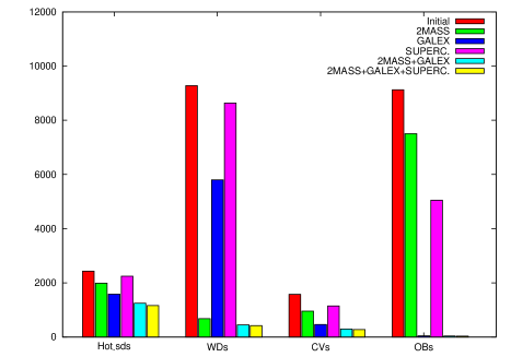
We selected only those targets having both 2mass and galex photometry, which significantly limited the test sample. Only a low fraction of the sample WDs has 2mass photometry since they are generally too faint at these wavelengths, while in the case of OB stars, there is galex photometry for very few targets since galex does not cover the galactic plane. Table 1 lists the number of targets with available photometric magnitudes for every input list (see also Fig. 1), and those having photometry in the two surveys (under 2mass+galex).

Table 1: Number of initial hot sds, WDs, CVs and OB targets used for defining the procedure in Section 3. The number of objects with available data in galex, 2mass and SuperCOSMOS is also included.

	Hot sds	WDs	CVs	OBs
Initial nums. in cats.	2430	9277	1578	9123
2mass	1985 (82%)	680 (7%)	956 (61%)	7504 (82%)
galex	1578 (65%)	5798 (62%)	460 (29%)	42 (0.46%)
SuperCOSMOS	2243 (92%)	8636 (93%)	1145 (73%)	5049 (55%)
2mass+galex	1246 (51%)	445 (5%)	292 (18%)	40 (0.44%)
2mass+galex+SuperC.	1162 (48%)	421 (4%)	274 (17%)	33 (0.36%)

galex and 2mass apparent magnitudes (FUV and NUV, and Ks, respectively) were corrected for galactic extinction using the $E(B-V)$ values from Schlegel et al. (1998) and applying the corresponding correction factors by Wyder et al. (2005) for FUV and NUV galex filters, and Cardelli et al. (1989) for the 2mass Ks filter:

$$FUV_{0}=FUV-A_{FUV}=FUV-8.376E(B-V)$$ (1)

$$NUV_{0}=NUV-A_{NUV}=NUV-8.741E(B-V)$$ (2)

$$Ks_{0}=Ks-A_{Ks}=Ks-0.114E(B-V)$$ (3)

where the $0$ subscripts indicate extinction corrected magnitudes.

Moreover, we also downloaded SuperCOSMOS, (Hambly et al. 2001) proper motions for the input list of targets, which will be used to separate different kinematic populations. A high fraction of the test objects have catalogued proper motions, as seen in Table 1. From now on, we will only use targets having 2mass and galex photometry and proper motions given by SuperCOSMOS (under 2mass+galex+SuperC in Table 1). This leaves us with a low fraction of WDs and a tiny fraction of OBs with respect to the original input catalogues, but we also lose about half of the initial hot sds.

Figure 1: Histogram showing the initial number of objects in the input catalogues, those with a counterpart in the databases used, and subsequent remaining numbers as cross-correlation between catalogues are done. Numbers are taken from Table 1.

3.2 Ultraviolet-infrared colour filter

Rhee et al. (2006) already presented a selection strategy to identify hot subdwarfs using a combination of photometric indices from galex and 2mass. The galex satellite is performing a series of sky surveys in two ultraviolet bands, FUV (1344 – 1786 Å) and NUV (1771 – 2831 Å), whereas 2mass scanned the entire sky in three near-infrared bands, J (1.25 $\mu$m), H (1.65 $\mu$m), and Ks (2.17 $\mu$m). Given their large area coverage, the combination of both datasets represents an excellent approach to separate blue from red targets.

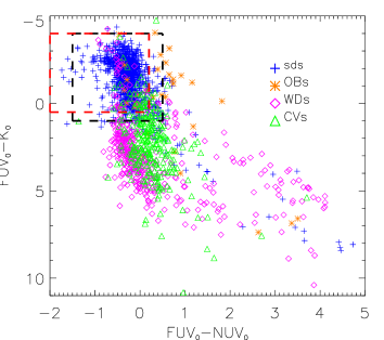
Rhee et al. (2006) cross-matched the galex and 2mass catalogues in a 3500 deg² region. They proposed as hot sds candidates those falling within the limits $-4<(FUV-Ks)<1$ and $-1.5<(FUV-NUV)<0.5$ in a two-colour diagram. However, follow-up spectroscopic observations for a subsample of 34 subdwarf candidates resulted in 60% contamination from other blue objects. We will therefore attempt to use slightly refined search criteria.

Following Rhee et al. (2006), we plotted $(FUV_{0}-Ks_{0})$ vs. $(FUV_{0}-NUV_{0})$ for the input sample (Fig. 2). The four different object classes under study are plotted with different colours and symbols. The black dashed box indicates the limits for the hot sds selection proposed by Rhee et al. (2006). It results in a very effective procedure to differentiate hot sds from the other samples: 92% of the considered hot sds lie within this box, while only 12% of the WDs, 24% of the CVs and 45% of the OBs fulfill this selection criterion.

Slight changes on the box limits result in a purer or more contaminated hot sds sample, always at the expense of sacrifying good candidates. After some tests, we redefined Rhee’s selection box as:

$$-4<(FUV_{0}-Ks_{0})<0.5$$ (4)

$$-2<(FUV_{0}-NUV_{0})<0.2$$ (5)

which is a good compromise between obtaining a low contamination factor and avoiding the rejection of too many hot sds. The new defined selection limits are overploted as a red dashed box in Fig. 2. Table 2 compares the percentage of targets surviving the two different selection criteria. As indicated, the new limits diminish contamination, in particular from CVs and OBs.

Given that white dwarfs can be nearby objects, their magnitudes might have been overcorrected for galactic extinction. As a cross-check, if half of the $E(B-V)$ values from Schlegel et al. (1998) were used, the resulting $FUV_{0}-K_{0}$ colours would be shifted towards blue $\sim 0.15$ mag on average, and only one new white dwarf would enter the selection criteria indicated in Fig. 2.

Figure 2: Test sample of hot sds, WDs, CVs and OBs having 2mass+galex+SuperCOSMOS data. Note that those hot sds with $FUV_{0}-NUV-0>2$ all have a $FUV$ magnitude above 18.7, close or above the limiting magnitude, which is causing their red appearance. The black dashed box comprises objects within the galex-2mass selection limits given by Rhee et al. (2006). The red dashed box gives selection limits proposed in this work. See text and Table 2 for further details.

Table 2: 1 & 2: Percentage of input objects fulfilling the selection criteria of two-colour indices $(FUV_{0}-Ks_{0})$ - $(FUV_{0}-NUV_{0})$ given by Rhee et al. (2006) and in this paper. 3: $H(NUV_{0})$ criterion proposed in this paper. Percentages refer to objects having data in 2mass+galex+SuperCOSMOS catalogues (see Table 1 for further details). 4: Absolute number of objects fulfilling criteria 2 & 3. 5: Percentage of objects with $T_{\rm eff}>$19 000 K; in parenthesis: considering also objects with a bad SED fit (see §3.4). 6: Same as 5, but in absolute numbers.

	Hot sds	WDs	CVs	OBs
1. Rhee et al. criteria
$-4<(FUV_{0}-Ks_{0})<1$	92%	12%	24%	45%
$-1.5<(FUV_{0}-NUV_{0})<0.5$
2. This paper
$-4<(FUV_{0}-Ks_{0})<0.5$	87%	10%	13%	33%
$-2<(FUV_{0}-NUV_{0})<0.2$
3. This paper
$19<H(NUV_{0})<27$	83%	3%	11%	21%
4. Total number after 2&3	960	14	30	7
5. VOSA $T_{\rm eff}>$19 000	64(72)%	3(3)%	1(4)%	3(6)%
6. Total number after 2,3,&5	749 (846)	14 (14)	3 (12)	1 (2)

3.3 Proper motion filter

Further improvement to this colour-colour diagram is obtained when reduced proper motions (RPM) are used to separate populations of stars with different kinematics. The RPM in any filter is calculated as:

$$H(Filter)=m+5\log_{10}(\mu)+5$$ (6)

where $m$ is the apparent magnitude for the corresponding filter and $\mu$ the proper motion measured in milliarcsec per year. Salim & Gould (2002) used a combination of optical and infrared RPMs to achieve a rather good isolation for the bluest WDs from main sequence stars and (cool) subdwarfs, although contamination factors were not given.

With this aim, we constructed an UV-RPM diagram for the test catalogues. In the upper panel of Fig. 3 we plotted H($NUV_{0}$) against ($FUV_{0}-NUV_{0}$) for the complete sample. Subdwarfs can be distinguished from OB main-sequence stars as they are several magnitudes dimmer at the same colour and typically have larger velocities. These effects tend to move hot sds significantly below the OB stars in the reduced proper-motion diagram. White dwarfs, with even fainter magnitudes, also appear clearly separated. Cataclysmic variables, on the other hand, quite overlap with hot sds and WDs.

Figure 3: Above: $H(NUV_{0})$ against $(FUV_{0}-NUV_{0})$ for the sample in Fig. 2. Notice inverted y-axis scale. Below: Only objects fulfilling Eqs. 4 and 5 are plotted (see §3.2). The red dashed box gives $H(NUV_{0})$ selection limits proposed in this work. See text and Table 2 for further details.

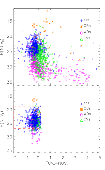
In the lower panel of Fig. 3 only targets fulfilling Eqs. 4-5 (see §3.2) are included. We now select targets within $19<H(NUV_{0})<27$, to end up with a sample almost devoid of WDs, containing only a 3% of the initial 2mass+galex+SuperCOSMOS selection, and a low fraction of the initial CVs (11%) and OBs (21%), as listed in Table 2 (point 3). Absolute numbers after application of these selection criteria are also included in Table 2 (point 4).

3.4 Spectral energy distribution fit

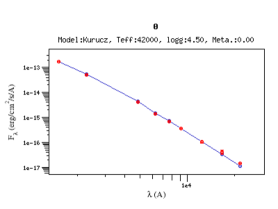
Finally, we obtained a temperature estimate for the surviving targets fitting their spectral energy distribution (SED). For this purpose, we employed the VO-tool VOSA (VO Sed Analyzer), which allows the user to query photometry from different catalogues, and compute $T_{\rm eff}$ from comparison of the SEDs with those derived from a grid of theoretical spectra.

We used the 2mass and galex photometry of the targets for the SED fit, as well as any photometric data existent in other public archives. With only 2mass and galex photometry it is difficult to get reliable values of the effective temperature due to: (i) 2mass photometry is not sensitive to $T_{\mathrm{eff}}$ changes within the typical temperature ranges for hot sds, i.e., large $T_{\mathrm{eff}}$ variations may still yield good fits and (ii) galex magnitudes are highly dependent on reddening and moderate errors in $E(B-V)$ translate into substantial errors in $T_{\mathrm{eff}}$.

In order to solve this problem we used VOSA to obtain photometry from the SDSS/DR7 (Abazajian et al. 2009), ukidss (Lawrence et al. 2007), CMC-14 and TYCHO-2 (Høg et al. 2000) services for the objects fulfilling the two-colour and RPM criteria (see point 4 in Table 2). The magnitudes are then transformed to fluxes and deredened using the extinction law by Fitzpatrick (1999). The observed SED is fit with a grid of Kurucz model atmospheres (Castelli et al. 1997) with ranges 3 500$<T_{\rm eff}<$50 000 K, 2.5$<\log g<$ 5.5. The temperature of the best fit for every object is represented in the histogram in Fig. 4. Note that this figure is shown in percentage for visibility reasons, given the low number of surviving objects other than hot sds.

Figure 4: Histogram showing the effective temperature distribution obtained with VOSA for the 960 hot sds (blue), 14 WDs (magenta), 30 CVs (green) and 7 OBs (orange). See text for details.

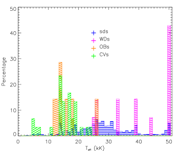
We can see in Fig. 4 that WDs have high scattered temperatures, as expected from them being in different stages of the cooling phase. We note that five WDs have a M dwarf companion, and for all of them we retrieve a $T_{\rm eff}$ estimate below 40 000 K. Concerning OBs and CVs, most of them are within 10–20 kK. When targets with the poorest goodness of fit are excluded of the plot, OBs and CVs’ location within 10–20 kK is emphasized. Therefore, we can use the temperature estimate given by VOSA to discard a large fraction of OB and CV objects.

We have adopted to discard as hot sds candidates, those objects with $T_{\rm eff}<$19 000 K and an acceptable goodness of fit, while we mantain as candidates those with $T_{\rm eff}>$19 000 K and those with bad fits, no matter their $T_{\rm eff}$. The reason for this last choice is that O-type hot sds can have effective temperatures exceeding Kurucz’s upper limit of 50 000 K and the fitting is expected to be poor for these hot objects. The implementation in VOSA of a set of NLTE sdO models hotter than 50.000 K is under investigation at the moment, to eventually be used in a further extension of our study. A poor fit may be also obtained for composite hot sds.

The results are included in Table 2: 72% of the initial hot sds survive all the selection filters imposed, while only 3%, 4% and 6% of the WDs, CVs and OBs are selected as candidates, which correspond to a very little fraction of contamination. It is difficult to asess the exact success rate, though, since the initial sample lists contain quite different number of objects.

4 Application of the method

In the previous section we designed a procedure to select a hot sds sample as pure as possible. In order to check the validity of this method, it was applied to two test sky regions and the results are described below.

4.1 Test region A: Kepler FoV

We tested our method in a region of about 420 deg², RA:(275,305) deg, DEC:(+33,+55) deg covering generously the Kepler FoV of 105 deg².

The Kepler FoV was chosen to test our method since extensive efforts are being made to select and classify suitable targets for long-term photometric monitoring. Within this framework, low-, intermediate- and high-resolution spectra of a large number of targets in the FoV are being acquired by different groups (Uytterhoeven et al. 2010). Indeed, we use the Kepler test region to be able to confirm our hot sds candidate list, thanks to the above mentioned works, without the necessity of performing our own spectroscopic observations.

Our workflow comprised the following steps:

1. Cross-match: For each galex source within the field, we looked for all 2mass counterparts in a 4 arcsec circular region. If more than one 2mass counterpart is found, then the galex source is removed.

2. Data filtering

   • We selected galex sources with FUV and NUV values brighter than the 5-$\sigma$ limiting magnitudes (19.9 and 20.8, respectively).

   • We dereddened galex (FUV, NUV) and 2mass (Ks) photometry using Eqs. 1-3 to obtain the corrected $FUV_{0},NUV_{0}$ and $Ks_{0}$.

   • We selected sources fulfilling $-4<(FUV_{0}-Ks_{0})<0.5$ and $-2<(FUV_{0}-NUV_{0})<0.2$. This step left us with 90 candidates.

   • We checked if the candidates were already in the catalogues used for defining the procedure (Section 3). After this step, 87 candidates remained

   • We retrieved SuperCOSMOS proper motions for the candidates using a 5 arcsec search radius and applied the RPM selection criteria ($19<H(NUV_{0})<27$). This yielded 73 candidates (see Table 7).

3. SED fitting: For each candidate, we used VOSA to obtain its effective temperature from the theoretical model that best fitted the observed SED. In this particular field it was necessary to download the photometry available in the Kepler Input Catalog(KIC) in order to perform an acceptable SED reconstruction, since only galex and 2mass data is retrieved from VO services.

   We thus restricted the analysis to those candidates with $g^{\prime}r^{\prime}i^{\prime}z^{\prime}$ SDSS photometry obtained during the Kepler preparatory programmes. This requisite limited our list to 21 objects, although we include in Table 7 the initial 73 candidates for general interest, and indicate the KIC number for these 21 targets with additional photometry in the KIC.

   From VOSA analysis, we selected those good fits having $T_{\rm eff}>$19 000 K, and those which were not correctly fitted regardless their temperature. After this step, we eventually ended up with 15 candidates. Table 3 gathers their photometry, while Fig. 5 includes the best SED fit for an example object.

Figure 5: Example of a SED fit performedy by VOSA for object (18:43:07,+42:59:18) in the Kepler FoV (see § 4.1 and Table 3).

Spectra were already available for all the candidates in Table 3 (Østensen et al. 2010c, 2011), from which we benefit to check the validity of our procedure. Thirteen of our candidates were classified as hot subdwarfs, the remaining objects being a main sequence B star and a DA star, which confirmed the robustness and efficiency of our method (87%).

Table 3 includes the spectral classification for the candidates, besides their corresponding KIC number. These 15 targets have all been already observed by Kepler, and Table 3 also indicates the survey cycle in which they were observed, and a brief description of their light curves.

4.2 Test region B: RA: 210-240; DEC:0-10

We also applied our procedure to a region of 300 deg²: RA: (210,240) deg, DEC:(0,10) deg following the steps enumerated in the previous section. We obtained a final list of 11 hot sds candidates, which are included in Table 4, together with their 2mass, galex and sdss photometry, along with $T_{\rm eff}$ estimated by VOSA and the spectral classification described below. For these objects we made use of Aladin to get the spectroscopic and catalogue data available in all Virtual Observatory services. The information is shown in Table 4 under column “Comments”.

Given that this region is covered by the Large Area Survey of ukidss, we repeated the workflow in the same field using the ukidss Data Release 7 instead of 2mass. Its large area coverage (7500 deg²) and depth (three magnitudes dimmer than 2mass) makes it very adequate to search for non-catalogued, faint hot sds, which may not be catalogued by 2mass. ukidss search yielded 12 additional candidates, which are listed in Table 5 with the same information as in Table 4.

Table 3: List of candidates in the Kepler field of view. FUV, NUV have been taken from the galex archive; $g^{\prime},r^{\prime},i^{\prime},z^{\prime}$ from the Kepler Input Catalogue and J,H,K from 2mass. “U” means upper limit in the 2mass photometry. $T_{\rm eff}$ is obtained from the best SED fit performed by VOSA. A bad SED fit is indicated with an (*) under “Comments”. KIC is the number from the Kepler input catalogue. Under “Comments” we include: the Kepler survey cycle in which each target was observed, a brief description of its light curve: (0): no particular features; (1): reflecting binary; (2): $g$-mode pulsator, (3): irregular variable, (4): variability from the companion; and the spectral classification: (A) from Østensen et al. (2010c) or (B): from Østensen et al. (2011)

RA	DEC	FUV	NUV	$g^{\prime}$	$r^{\prime}$	$i^{\prime}$	$z^{\prime}$	J	H	K	$T_{\rm eff}$	Class.	KIC	Comments
(J2000)	(J2000)										(VOSA)		number
18:42:42	+44:04:06	16.317	16.442	17.056	17.378	17.555	17.630	16.75	16.34	15.78	25 000	sdB	8142623	(*)$Q_{1}$ (1)(A)
18:43:07	+42:59:18	14.149	14.737	15.410	15.864	16.208	16.528	16.27	16.13	U:16.24	42 000	sdO+dM	7335517	$Q_{3}$ (1)(B)
18:47:14	+47:41:47	13.305	13.772	14.489	14.988	15.366	15.725	15.39	15.62	15.47	41 000	He-sdO	10449976	$Q_{3}$ (0)(B)
18:50:17	+43:58:29	16.501	16.387	16.353	16.649	16.996	17.115	16.71	U:17.15	U:17.00	23 000	B	8077281	$Q_{2}$ (3)(A)
19:04:35	+48:10:22	15.726	16.057	16.696	17.031	17.236	17.456	16.63	U:16.34	U:17.11	25 000	sdB	10784623	$Q_{5}$(1)(B)
19:05:06	+43:18:31	14.208	14.391	15.058	15.516	15.894	16.193	15.81	16.06	U:16.23	30 000	sdB	7668647	$Q_{3}$ (2)(B)
19:08:25	+45:08:32	15.267	15.518	16.283	16.605	16.755	16.819	16.17	15.78	15.36	26 000	sdB	8874184	(*)$Q_{4}$(4)(B)
19:08:46	+42:38:31	13.983	14.490	15.146	15.595	15.964	16.295	15.90	16.05	16.02	35 000	sdB	7104168	$Q_{3}$ (0)(B)
19:09:33	+46:59:04	14.695	15.009	15.483	15.967	16.308	16.607	16.36	U:15.71	U:16.61	35 000	sdB	10001893	$Q_{3}$ (2)(B)
19:10:00	+46:40:24	14.119	14.496	14.572	14.583	14.613	14.672	13.93	13.80	13.73	18 000	sdO+F/G	9822180	(*)$Q_{2}$(4)(A)
19:14:28	+45:39:09	15.002	15.339	15.895	16.174	16.297	16.423	16.02	15.57	15.68	26 000	sdB	9211123	$Q_{3}$ (0)(B)
19:16:12	+47:49:16	15.291	15.413	15.269	15.278	15.339	15.351	14.62	14.42	14.27	15 000	sdB+F/G	10593239	(*)$Q_{2,5}$(4$?$)(A)
19:26:51	+49:08:48	14.981	14.813	15.396	15.522	15.565	15.595	14.83	14.52	14.37	21 000	sdB+F/G	11350152	(*)$Q_{3}$ (4)(B)
19:40:32	+48:27:23	13.544	13.969	14.093	14.175	14.269	14.369	13.68	13.56	13.56	20 000	sdB+F/G	10982905	(*)$Q_{2}$ (4)(A)
19:43:44	+50:04:38	13.228	13.888	14.455	14.938	15.320	15.682	15.37	15.36	15.18	50 000	DA	11822535	(*)$Q_{2}$ (0)(A)

Table 4: List of candidates in the Test Region B obtained from the galex-2mass-SuperC cross-match. FUV, NUV have been taken from the galex archive; $u,g,r,i,z$ from the SDSS Data Release 7 and J,H,K from the 2mass Point Source Catalogue.“U” means upper limit in the 2mass photometry. $T_{\rm eff}$ is obtained from the best SED fit performed by VOSA. Under “Comments“: known names are given when possible; (*) indicates a bad VOSA fitting; (1): catalogued in Østensen et al. (2010b); (2): classified as DA by Koester et al. (2009).

RA	DEC	FUV	NUV	$u$	$g$	$r$	$i$	$z$	J	H	K	$T_{\rm eff}$	Class.	Comments
(J2000)	(J2000)											(VOSA)
14:14:35	+00:12:36	14.378	14.770	15.389	15.725	16.240	16.585	16.921	16.46	U:16.37	U:16.81	480̇00		FBS 1412+004
14:23:40	+00:10:21	16.074	16.669	17.469	17.854	18.065	17.914	17.683	16.19	15.57	15.58	44 000
14:58:06	+08:51:30	13.886	14.282	14.380	14.349	14.839	15.160	15.474	15.14	15.11	15.01	23 000	sdB
15:10:42	+04:09:55	15.838	15.962	16.541	16.810	17.249	17.498	17.692	16.72	U:16.26	U:16.45	31 000	sdOB	(1) J15104+0409
15:16:46	+09:26:32	15.857	16.285	16.854	17.019	17.295	17.452	17.641	16.57	16.26	U:16.06	19 000	sdB+F/G
15:35:10	+03:11:14	14.020	14.727	24.109	15.636	16.148	16.517	16.851	16.48	16.42	U:17.16	50 000	DA	(*,2) WD1532+033
15:43:39	+00:12:02	16.204	16.437	16.708	16.726	17.027	17.169	17.325	16.71	16.26	U:15.44	23 000	sdB	(1) EGGR 491
15:45:46	+01:32:29	16.297	16.690	16.901	16.673	16.580	16.525	16.512	15.62	15.10	14.99	21 000	sdB+F/G	(*)
15:51:20	+06:49:04	15.362	15.591	15.987	15.891	15.936	15.949	15.988	15.26	14.98	14.90	8 000	sdOB+X	(*,1) J15513+0649
15:53:33	+03:44:34	16.533	16.785	16.618	16.688	16.828	16.913	17.018	16.29	16.03	15.54	24 000	He-sdOB
15:56:28	+01:13:35	15.338	15.633	15.867	15.985	16.387	16.707	16.935	16.46	16.63	U:17.02	29 000	sdB	(1) J15564+01131

Table 5: List of candidates in Test Region B obtained from the galex-UKIDSS-SuperC cross-match. FUV, NUV have been taken from the galex archive; $u,g,r,i,z$ from the SDSS Data Release 7 and Y,J,H,K from the ukidss Large Area Survey (DR7). $T_{\rm eff}$ is obtained from the best SED fit performed by VOSA. Under “Comments”: (*) indicates a bad VOSA fitting; (1) catalogued in McCook & Sion (1999); (2) classified as sdB in Eisenstein et al. (2006); (3) classified as sdO in Eisenstein et al. (2006)

RA	DEC	FUV	NUV	$u$	$g$	$r$	$i$	$z$	Y	J	H	K	$T_{\rm eff}$	Class	Comments
(J2000)	(J2000)												(VOSA)
14:15:17	+09:49:26	17.485	17.968	18.765	19.150	19.493	19.317	18.958	18.267	17.804	17.298	17.003	7 200		(*)
14:24:37	+02:34:19	15.712	16.118	16.465	16.464	16.841	17.122	16.986	17.060	17.129	17.220	17.245	23 000	DA	(1) PG1422+028
14:34:40	+06:07:03	15.988	16.524	17.288	17.714	18.175	18.258	18.140	17.508	17.142	16.633	16.458	39 000
14:39:18	+01:02:51	16.326	16.285	16.391	16.367	16.769	17.060	17.340	16.968	17.054	17.139	17.216	21 000	sdB	(2) J1439+0102
14:47:30	+03:15:06	16.049	16.222	16.311	16.137	16.550	16.855	17.108	16.748	16.740	16.698	16.809	20 000
15:02:30	+09:13:57	16.190	16.354	16.935	17.256	17.763	18.119	18.489	18.117	18.220	18.418	18.529	39 000	sdOB
15:25:34	+09:58:51	16.207	16.471	17.065	17.353	17.829	18.102	18.331	17.977	17.887	17.634	17.625	31 000	sdOB
15:26:08	+00:16:41	15.026	15.603	16.185	16.573	17.066	17.436	17.787	17.489	17.514	17.633	17.656	50 000	He-sdOB	(3) J1526+0016
15:27:04	+08:02:37	16.920	17.223	17.748	17.839	18.194	18.397	18.679	18.161	18.195	18.118	17.883	19 000
15:28:52	+09:31:44	15.059	15.374	15.920	16.161	16.664	17.030	17.340	17.046	17.148	17.223	17.345	34 000	sdOB
15:35:25	+06:56:52	15.479	15.656	16.044	16.173	16.643	16.949	17.266	16.921	17.012	17.020	17.070	27 000
15:38:34	+03:08:13	15.718	15.932	16.449	16.686	17.169	17.507	17.824	17.488	17.572	17.645	17.796	34 000

4.2.1 Spectroscopic follow-up

While all hot sd candidates from test region A were already classified, this is not the case for test region B, where only a few objects are identified in the literature, as explained below. For this reason, we have performed spectroscopic follow-up for candidates from test region B, which is described in what follows.

Test region B: 2mass-galex: Five objects from Table 4 have an available SDSS spectrum. Four of them (J15104+0409, EGGR 491, J15513+0649, J15564+01131) are classified as hot subdwarfs in Østensen et al. (2010b), while a visual inspection of the fifth object ((15:53:33,+03:44:34), see Fig. 6) confirms it is also a hot subdwarf. On the other hand, Koester et al. (2009) classify WD 1532+033 as a DA object.

Follow-up spectroscopy of 3 additional objects from Table 4 could be gathered at the Isaac Newton Telescope (INT) and the William Herschell Telescope (WHT) in La Palma (Spain) as a filling program. The IDS spectrograph mounted on the INT was used with the R400B grating providing a resolution of R$\approx$1400 and an effective wavelength coverage $\lambda\backsimeq$3100–6700 Å. The ISIS spectrograph was used in the case of the WHT with grating R300B on the blue arm (R$\approx$1600, $\lambda\backsimeq$3100–5300 Å). Standard IRAF packages were used for the data reduction, which included bias subtraction, flatfield correction and wavelength calibration. The extracted spectra were normalized to obtain a raw spectral classification in order to check the success rate of our methodology. The normalized spectra of these objects are included in Fig. 6.

Figure 6: Follow-up spectroscopy gathered at the INT and WHT for some candidates of Table 4, and SDSS spectra that were available for some others from Tables 4,5 (last four panels). The first Balmer lines are indicated as dotted vertical lines; dashed vertical lines indicate HeI spectral lines; HeII4686 is marked with a dashed-dotted line; the G-band is also indicated when present.

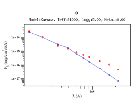
The first object (14:58:06,+08:51:30) displays a typical sdB spectrum, with only broad Balmer lines up to a low series number. The Caii H and K lines may indicate an sdB star with an F or G type companion, but may also be caused by a significant amount of dust along the line of sight. The Caii H line, when present, deepens the $H_{\epsilon}$ line, and is often used as an indicator of sdB+F/G composites. The second object in Fig. 6, (15:16:46,+09:26:32), seems to be a case of such an sdB+F/G composite. The spectrum of (15:45:46,+01:32:29) is noisier, but the G-band together with the deep $H_{\epsilon}$ line hints towards a composite nature for this star too. When taken together with the distinctive red excess seen in the SED (Fig. 7), the composite nature of this object is quite certain. Modelling this object with two Kurucz components provides an excellent fit, as illustrated in the lower panel of Fig. 7. The optimum fit is achieved for a hot+cool pair with temperatures 30 000+5 000K and a radius ratio $R_{\rm cool}/R_{\rm hot}\simeq 8$.

The SDSS spectrum of object (15:53:33,+03:44:34) is also included in Fig. 6, which is identified as a He-sdOB based on the presence of Balmer, HeI and HeII lines.

Note that we use the same classification scheme as in Østensen et al. (2010c), in which a distinction is made between the common He-sdOB stars showing HeI and HeII with almost equal depth, and the hotter and more scarce He-sdOs, with predominantly HeII lines.

Test region B: ukidss-galex: We were unable to perform any follow-up spectroscopy for candidates in Table 5 due to their faintness. However, one object is classified as WD DA by McCook & Sion (1999) (PG1422+028), and two objects are identified as hot sds by Eisenstein et al. (2006) (J1439+0102: sdB; J1526+0016: sdO). Moreover, three other targets have an SDSS spectrum: (15:02:30,+09:13:57), (15:25:34,+09:58:51), (15:28:52,+09:31:44), and we also include them in Fig. 6 at the bottom. The three have very similar spectra, displaying some HeI lines: 4027,4471 Å (and 4922 Å in the case of (15:28:52,+09:31:44)) plus the HeII4686 line (only traces for (15:28:52,+09:31:44)) in addition to the Balmer serie. We classify all of them as sdOB objects, as indicated in Table 5.

5 Binary hot subdwarfs in the sample

In the lists of candidates of both test region A and B (Tables 3,4,5), we have indicated with an asterisk those targets for which a bad SED fit is obtained. A bad fit is expected to occur for objects hotter than $T_{\rm eff}>$50 000 K (the hot end of the Kurucz grid used), as this seems to happen for the white dwarfs (19:43:44,+50:04:38) in Table 3 and (15:35:10,+03:11:14) in Table 4.

In case a target is in a binary system with a cool companion, its impact at long wavelengths can also cause a bad SED fit. We have encountered 9 such cases with a more or less clear infrared excess that may be due to a red companion. For these cases, we have fitted the spectral distribution to a combination of two Kurucz model atmospheres. In Fig. 7 we can see how a two-components fit (lower panel) gives a much better match to the observed spectral distribution compared to a single-component fit (upper panel) for object (15:45:46,+01:32:29). The temperatures of the best hot+cool pair for the nine cases are included in Table 6. Only for two targets, the two-components fit did not improve the single-component one performed by VOSA; for them no temperatures are included in the table and further analyses will be foreseen for these two objects.

Figure 7: Upper: best VOSA SED fit for the object (15:45:46,+01:32:29). It displays the G-band in the spectrum (see Fig. 6), and an infrared excess in the spectral distribution. Bottom: best fit obtained considering two Kurucz components.

Table 6: Two components SED decomposition for objects with a bad fit in Tables 3,4,5 (marked with an asterisk under ”Comments“), which may be due to a cool companion. Only for objects (18:42:42 ,+44:04:06) and (19:08:25,+45:08:32) the two-components fit does not improve the single-component one.

Object	$T_{\rm eff}$ hot	$T_{\rm eff}$ cool
18:42:42 +44:04:06	—	—
19:08:25 +45:08:32	—	—
19:10:00 +46:40:24	37 000	6 250
19:16:12 +47:49:16	22 000	5 250
19:26:51 +49:08:48	28 000	5 000
19:40:32 +48:27:23	31 000	5 750
15:45:46 +01:32:29	30 000	5 000
15:51:20 +06:49:04	29 000	5 500
14:15:17 +09:49:26	29 000	5 500

6 Conclusions

We have developed a methodology to find new uncatalogued hot subdwarfs making use of large databases such as galex, 2mass, ukidss and SuperCOSMOS. VO tools helped to handle the different queries and the large output list of candidates. We tested the methodology using bona-fide input objects from the literature, which are spectroscopically classified in the catalogues listed in Section 3.

The 2mass-galex photometry combination is first used to separate blue objects from redder ones. A selection criterion given by Eqs. 4,5 effectively retrieves hot sd candidates, along with other UV-excess objects: mainly white dwarfs, cataclysmic variables and main sequence OB stars. 87% of the input hot sds, while only 10%, 13% and 33% of the input WDs, CVs and OB stars survive this first filter. Using reduced proper motions, the hot sd selection further improves, with very few WDs fulfilling the adopted proper motion criterion (see Table 2).

Moreover, the Virtual Observatory Sed Analyzer (VOSA) was used to obtain a rough guess of temperatures for the candidates. These are computed fitting Kurucz model atmospheres to the spectral energy distribution, constructed using all the available photometry for every target. We adopt as hot sds threshold objects with $T_{\rm eff}>$19 000 K. This criterion is specially useful to filter out CVs and OB stars, since, in general, lower temperatures are obtained by VOSA for these objects (see Fig. 4). Targets with a bad fit are retained as good candidates independently of their temperature estimate, given that a poor fit may be obtained for stars showing infrared excess indicative of a cool companion, or for sdOs of high temperature ($T_{\rm eff}>$50 000 K).

After all these filters are imposed, 72% of the initial hot sds remain, while, on the other hand, only a low fraction of other spectral types meet the criteria adopted: 3%, 4% and 6% of the initial WDs, CVs and OBs respectively.

We have applied this strategy to two test regions: a $\sim$420 deg² region centered on the Kepler satellite field of view (test region A), and other at RA:210–240, DEC:0–10 (test region B). In the Kepler FoV, 73 objects fulfill the colour and proper motion criteria. However, only 21 have additional KIC $g^{\prime}r^{\prime}i^{\prime}z^{\prime}$ photometry besides 2mass and galex, which is necessary to perform an acceptable SED fit. Thirteen of them have temperature estimates above 19 000 K and two are retained because of its bad fit (see Table 3). Thanks to the ground-based support to the Kepler mission, spectroscopic follow-up of all the candidates was available. Thirteen candidates are confirmed to be hot sds, with only two targets contaminating the sample: a main sequence B star, and a white dwarf.

For test region B, we applied the same methodology, and obtained a list of 11 candidates (see Table 4), 3 of them retained due to a bad SED fit. Four of these objects have been recently classified as hot sds by Østensen et al. (2010b), a fifth target is classified as DA by Koester et al. (2009), and a sixth candidate (15:53:33,+03:44:34) has an spectrum in the SDSS database, which identifies the object as a hot sd. Follow-up spectroscopy could be acquired for 3 other objects at the INT and WHT (La Palma). The classification is included in Table 4.

Furthermore, we repeated the same procedure for test region B, but using ukidss instead of the 2mass database. 12 candidates are proposed, out of which 2 are classified as hot sds by Eisenstein et al. (2006), one is labeled as DA by McCook & Sion (1999) and 3 are identified as hot sds in this paper based on available Sloan spectra (see Fig. 6).

In total, we proposed 38 candidates, of which 30 could be spectroscopically classified, and 26 of them were confirmed to be hot sds. The success rate is thus 87%. This high percentage confirms the suitability of our methodology to discover new hot subdwarfs.

Former surveys described in §2 aimed at finding faint blue stars in general and not only hot subdwarfs in particular. Thus, it is intrinsically improper to compare our finding rate with the percentage of hot sds found in these works. However, they rate a maximum of 53% of hot sds and demonstrate the difficulty of this task due to the photometric (and spectroscopic) similitudes among blue objects.

Østensen et al. (2010c, 2011) compile the variety of methods used by several teams to obtain uncatalogued blue compact targets within the Kepler FoV. Most of the methods are based only on photometric colours and do not particularly intend to discern white dwarfs from hot sds, since both classes are of interest from a seismological point of view. Their success rate ranges from poor, when only 2mass colours are considered, to actually very good, when using SDSS filters. The complete sample listed in  Østensen et al. (2010c, 2011) is formed by 68 sds, 17 WDs, 14 Bs, 2 PNN, 3 CVs and 6 other main sequence stars. Comparing with the number of hot sds candidates proposed in this work, only 19 of the 68 hot sds in Østensen et al. (2010c, 2011) have all the necessary data required by our methodology (2mass, galex and proper motion), 17 of which fulfill all our selection criteria. We have retrieved 13 of them; for the other 4 hot sds, their galex photometry is obtained from the Guest Investigator survey, which was not public at the time our search was performed, and thus these targets are not listed as candidates in Table 3. This serves as a cross-check that: i) a low fraction of hot sds are rejected by our search method, as expected from the tests made in Section 3, and ii) that we will be able to increase our detections as the sky is better covered by the large surveys we make use of.

We note that the use of proper motion data was particularly suitable for finding WDs, as described in Østensen et al. (2010c, 2011). Proper motion information has also been useful to spot WDs and hot sds by Jiménez-Esteban et al. (2011), whose objective is the identification of blue high proper motion objects.Combined photometric indexes and proper motion data is also employed by Vennes et al. (2010) with the intention of finding new white dwarfs. Their bright sample of candidates contains one single (and already known) WD, plus 15 hot sds (6 already catalogued), 29 main sequence B stars and other 5 blue objects of different nature.

Encouraged by the results in the two pilot regions, and taking advantage of the Virtual Observatory capabilities, we have initiated a systematic search for hot subdwarf stars in the Milky Way, the results of which will be published in a forthcoming paper.

Table 7: List of the 73 candidates in and around the Kepler field of view that fulfill the photometric and proper motion criteria. FUV, NUV have been taken from the galex archive and J,H,K from 2mass. The KIC number for 21 objects with additional photometry is included. (*) indicates objects meeting all the selection criteria, detailed in Table 3.

RA	DEC	FUV	NUV	J	H	K	KIC		RA	DEC	FUV	NUV	J	H	K	KIC
(J2000)	(J2000)						number		(J2000)	(J2000)						number
18:19:48	+33:22:09	15.704	15.745	17.02	17.04	16.48			18:50:46	+51:07:38	14.416	14.134	14.01	14.10	14.17
18:20:55	+33:18:47	16.137	16.291	17.03	16.63	17.47			18:57:58	+44:40:57	16.300	16.454	15.79	15.63	15.40	8544347
18:20:58	+37:07:07	14.441	14.658	16.49	15.89	16.53			19:03:44	+47:24:39	14.991	15.303	15.45	14.94	14.93
18:21:10	+34:46:45	13.062	14.152	15.29	15.50	15.47			19:04:35	+48:10:22	15.726	16.057	16.63	16.34	17.11	10784623 (*)
18:21:50	+41:51:56	16.438	16.870	16.79	16.80	15.87			19:05:06	+43:18:31	14.208	14.391	15.81	16.06	16.23	7668647 (*)
18:22:43	+43:20:37	12.865	13.110	14.40	14.52	14.50			19:05:20	+44:57:59	17.545	17.594	16.41	15.93	17.28	8741434
18:23:10	+33:33:55	14.461	14.451	15.66	15.56	15.99			19:08:25	+45:08:32	15.267	15.518	16.17	15.78	15.36	8874184 (*)
18:23:57	+41:29:14	13.682	13.653	15.16	15.29	15.64			19:08:46	+42:38:32	13.983	14.490	15.90	16.05	16.02	7104168 (*)
18:24:00	+51:55:25	14.362	14.801	16.25	16.08	15.94			19:09:20	+45:40:57	14.295	14.622	14.72	14.87	14.88
18:24:08	+35:16:19	14.767	15.129	15.41	15.11	14.97			19:09:34	+46:59:04	14.695	15.009	16.36	15.71	16.61	10001893 (*)
18:24:34	+38:00:54	15.723	15.811	16.39	16.94	15.74			19:10:00	+46:40:25	14.119	14.496	13.93	13.80	13.73	9822180 (*)
18:24:44	+35:30:42	14.218	14.603	16.83	16.64	17.33			19:10:24	+47:09:45	11.796	12.368	11.31	11.45	11.47	10130954
18:24:49	+38:51:38	14.516	14.947	16.15	16.31	15.67			19:14:28	+45:39:11	15.002	15.339	16.02	15.57	15.68	9211123 (*)
18:25:19	+40:33:34	15.010	15.139	16.26	16.43	16.76			19:15:08	+47:54:20	13.617	14.043	13.30	13.33	13.36	10658302
18:26:22	+32:51:08	14.236	14.637	15.54	16.18	15.25			19:16:12	+47:49:16	15.291	15.413	14.62	14.42	14.27	10593239 (*)
18:26:37	+34:37:26	14.578	14.714	16.40	16.46	17.34			19:20:03	+49:15:33	15.392	15.567	16.76	16.29	15.84
18:27:45	+37:09:31	16.518	16.700	16.48	16.42	16.06			19:20:18	+48:06:21	15.655	15.873	16.74	17.19	16.25
18:27:55	+36:22:08	14.688	14.938	16.60	15.86	16.13			19:20:36	+49:03:16	14.275	14.500	13.50	13.49	13.54	11293898
18:28:50	+34:36:50	14.217	14.627	16.55	15.70	16.14			19:26:52	+49:08:49	14.981	14.813	14.83	14.52	14.37	11350152 (*)
18:32:21	+55:03:00	15.117	15.713	15.50	14.85	14.83			19:30:49	+54:21:28	16.309	16.531	16.62	16.28	16.57
18:33:44	+43:01:06	15.482	15.580	16.49	16.40	16.71			19:36:33	+52:45:19	16.609	17.221	16.74	15.97	15.42
18:34:54	+44:49:17	14.607	14.726	13.85	13.63	13.51			19:40:32	+48:27:24	13.544	13.969	13.68	13.56	13.56	10982905 (*)
18:35:17	+43:27:30	14.230	14.219	14.26	14.22	14.14			19:43:44	+50:04:39	13.228	13.888	15.37	15.36	15.18	11822535 (*)
18:36:21	+40:59:38	14.974	15.221	13.98	13.87	13.79			19:44:43	+54:49:43	15.654	15.748	16.11	16.01	15.83
18:36:34	+53:16:57	12.861	13.589	12.74	12.79	12.84			19:50:24	+50:09:00	15.583	15.587	13.61	13.60	13.68
18:36:42	+41:30:46	15.252	15.477	15.08	14.91	14.97			19:53:04	+49:49:34	15.581	15.923	16.32	16.23	15.62
18:39:49	+53:00:04	14.797	15.050	16.67	16.01	15.98			19:53:42	+49:59:45	14.713	15.329	16.47	16.27	16.47
18:40:21	+41:43:15	15.376	15.386	15.24	15.24	15.11			19:54:52	+48:22:29	15.014	14.920	13.95	13.96	13.99	10937527
18:42:03	+45:31:59	14.883	14.842	14.56	14.62	14.55			19:56:48	+53:12:17	15.413	15.941	15.27	14.76	14.54
18:42:42	+44:04:05	16.317	16.442	16.75	16.34	15.78	8142623 (*)		19:57:28	+53:32:03	13.989	14.650	14.47	14.19	14.02
18:43:07	+42:59:18	14.149	14.737	16.27	16.13	16.24	7335517 (*)		20:00:01	+54:09:03	15.202	15.155	12.55	12.54	12.52
18:43:56	+45:37:57	15.009	15.204	16.75	16.90	16.79			20:01:54	+49:03:54	15.119	15.456	16.44	15.74	17.05
18:47:14	+47:41:47	13.305	13.772	15.39	15.62	15.47	10449976 (*)		20:06:33	+48:33:29	12.383	13.752	9.14	9.11	9.08
18:47:46	+50:41:35	13.877	14.061	15.24	15.45	15.94			20:07:39	+54:45:16	17.424	17.667	16.81	16.29	15.84
18:49:15	+51:16:05	13.792	13.941	15.54	15.58	15.09			20:09:34	+55:05:25	18.663	18.538	15.76	15.52	15.44
18:50:05	+50:24:22	15.206	15.315	14.60	14.52	14.39			20:11:52	+54:50:11	14.201	13.914	10.11	10.05	10.02
18:50:17	+43:58:29	16.501	16.387	16.71	17.15	17.00	8077281 (*)

References

- Abazajian et al. (2009) Abazajian, K. N., Adelman-McCarthy, J. K., Agüeros, M. A., et al. 2009, ApJS, 182, 543
- Altmann et al. (2004) Altmann, M., Edelmann, H., & de Boer, K. S. 2004, A&A, 414, 181
- Auvergne et al. (2009) Auvergne, M., Bodin, P., Boisnard, L., et al. 2009, A&A, 506, 411
- Bauer & Husfeld (1995) Bauer, F. & Husfeld, D. 1995, A&A, 300, 481
- Borucki et al. (2010) Borucki, W. J., Koch, D., Basri, G., et al. 2010, Science, 327, 977
- Cardelli et al. (1989) Cardelli, J. A., Clayton, G. C., & Mathis, J. S. 1989, ApJ, 345, 245
- Castelli et al. (1997) Castelli, F., Gratton, R. G., & Kurucz, R. L. 1997, A&A, 318, 841
- Charpinet et al. (2010) Charpinet, S., Green, E. M., Baglin, A., et al. 2010, A&A, 516, L6
- Chavira (1958) Chavira, E. 1958, Boletin de los Observatorios Tonantzintla y Tacubaya, 2, 15
- D’Cruz et al. (1996) D’Cruz, N. L., Dorman, B., Rood, R. T., & O’Connell, R. W. 1996, ApJ, 466, 359
- Demers et al. (1986) Demers, S., Beland, S., Kibblewhite, E. J., Irwin, M. J., & Nithakorn, D. S. 1986, AJ, 92, 878
- Dorman et al. (1993) Dorman, B., Rood, R. T., & O’Connell, R. W. 1993, ApJ, 419, 596
- Downes (1986) Downes, R. A. 1986, ApJS, 61, 569
- Downes et al. (2006) Downes, R. A., Webbink, R. F., Shara, M. M., et al. 2006, VizieR Online Data Catalog, 5123, 0
- Dreizler et al. (1990) Dreizler, S., Heber, U., Werner, K., Moehler, S., & de Boer, K. S. 1990, A&A, 235, 234
- Edelmann et al. (2003) Edelmann, H., Heber, U., Hagen, H., et al. 2003, A&A, 400, 939
- Eisenstein et al. (2006) Eisenstein, D. J., Liebert, J., Harris, H. C., et al. 2006, ApJS, 167, 40
- Feige (1958) Feige, J. 1958, ApJ, 128, 267
- Fitzpatrick (1999) Fitzpatrick, E. L. 1999, PASP, 111, 63
- Fontaine et al. (2008) Fontaine, G., Brassard, P., Green, E. M., et al. 2008, A&A, 486, L39
- For et al. (2010) For, B., Green, E. M., Fontaine, G., et al. 2010, ApJ, 708, 253
- Green et al. (1986) Green, R. F., Schmidt, M., & Liebert, J. 1986, ApJS, 61, 305
- Greenstein (1960) Greenstein, J. L., ed. 1960, Stellar atmospheres.
- Greenstein (1966) Greenstein, J. L. 1966, ApJ, 144, 496
- Hagen et al. (1995) Hagen, H., Groote, D., Engels, D., & Reimers, D. 1995, A&AS, 111, 195
- Hambly et al. (2001) Hambly, N. C., Davenhall, A. C., Irwin, M. J., & MacGillivray, H. T. 2001, MNRAS, 326, 1315
- Han et al. (2003) Han, Z., Podsiadlowski, P., Maxted, P. F. L., & Marsh, T. R. 2003, MNRAS, 341, 669
- Han et al. (2002) Han, Z., Podsiadlowski, P., Maxted, P. F. L., Marsh, T. R., & Ivanova, N. 2002, MNRAS, 336, 449
- Haro & Luyten (1962) Haro, G. & Luyten, W. J. 1962, Boletin de los Observatorios Tonantzintla y Tacubaya, 3, 37
- Heber (1986) Heber, U. 1986, A&A, 155, 33
- Heber et al. (1991) Heber, U., Jordan, S., & Weidemann, V. 1991, in NATO ASIC Proc. 336: White Dwarfs, ed. G. Vauclair & E. Sion, 109
- Høg et al. (2000) Høg, E., Fabricius, C., Makarov, V. V., et al. 2000, A&A, 355, L27
- Humason & Zwicky (1947) Humason, M. L. & Zwicky, F. 1947, ApJ, 105, 85
- Iriarte & Chavira (1957) Iriarte, B. & Chavira, E. 1957, Boletin de los Observatorios Tonantzintla y Tacubaya, 2, 3
- Jiménez-Esteban et al. (2011) Jiménez-Esteban, F. M., Caballero, J. A., & Solano, E. 2011, A&A, 525, A29
- Kilkenny et al. (1988) Kilkenny, D., Heber, U., & Drilling, J. S. 1988, South African Astronomical Observatory Circular, 12, 1
- Kilkenny et al. (2010) Kilkenny, D., O’Donoghue, D., Hambly, N., & MacGillivray, H. 2010, Ap&SS, 86
- Kilkenny et al. (1997) Kilkenny, D., O’Donoghue, D., Koen, C., Stobie, R. S., & Chen, A. 1997, MNRAS, 287, 867
- Koester et al. (2009) Koester, D., Voss, B., Napiwotzki, R., et al. 2009, A&A, 505, 441
- Lamontagne et al. (2000) Lamontagne, R., Demers, S., Wesemael, F., Fontaine, G., & Irwin, M. J. 2000, AJ, 119, 241
- Lawrence et al. (2007) Lawrence, A., Warren, S. J., Almaini, O., et al. 2007, MNRAS, 379, 1599
- Maxted et al. (2001) Maxted, P. f. L., Heber, U., Marsh, T. R., & North, R. C. 2001, MNRAS, 326, 1391
- McCook & Sion (1999) McCook, G. P. & Sion, E. M. 1999, ApJS, 121, 1
- Mengel et al. (1976) Mengel, J. G., Norris, J., & Gross, P. G. 1976, ApJ, 204, 488
- Morales-Rueda et al. (2003) Morales-Rueda, L., Maxted, P. F. L., Marsh, T. R., North, R. C., & Heber, U. 2003, MNRAS, 338, 752
- Morrissey et al. (2007) Morrissey, P., Conrow, T., Barlow, T. A., et al. 2007, ApJS, 173, 682
- Napiwotzki et al. (2003) Napiwotzki, R., Christlieb, N., Drechsel, H., et al. 2003, The Messenger, 112, 25
- Napiwotzki et al. (2004) Napiwotzki, R., Karl, C. A., Lisker, T., et al. 2004, Ap&SS, 291, 321
- Østensen (2006) Østensen, R. H. 2006, Baltic Astronomy, 15, 85
- Østensen et al. (2010a) Østensen, R. H., Green, E. M., Bloemen, S., et al. 2010a, MNRAS, L126
- Østensen et al. (2010b) Østensen, R. H., Oreiro, R., Solheim, J., et al. 2010b, A&A, 513, A6
- Østensen et al. (2011) Østensen, R. H., Silvotti, R., Charpinet, S., et al. 2011, MNRAS
- Østensen et al. (2010c) Østensen, R. H., Silvotti, R., Charpinet, S., et al. 2010c, MNRAS, 409, 1470
- Randall et al. (2009) Randall, S. K., van Grootel, V., Fontaine, G., Charpinet, S., & Brassard, P. 2009, A&A, 507, 911
- Reed (2005) Reed, C. 2005, VizieR Online Data Catalog, 5125, 0
- Rhee et al. (2006) Rhee, J., Seibert, M., Østensen, R. H., et al. 2006, Baltic Astronomy, 15, 77
- Rodríguez-López et al. (2010) Rodríguez-López, C., Lynas-Gray, A. E., Kilkenny, D., et al. 2010, MNRAS, 401, 23
- Rodríguez-López et al. (2007) Rodríguez-López, C., Ulla, A., & Garrido, R. 2007, MNRAS, 379, 1123
- Salim & Gould (2002) Salim, S. & Gould, A. 2002, ApJ, 575, L83
- Sargent & Searle (1968) Sargent, W. L. W. & Searle, L. 1968, ApJ, 152, 443
- Schlegel et al. (1998) Schlegel, D. J., Finkbeiner, D. P., & Davis, M. 1998, ApJ, 500, 525
- Skrutskie et al. (2006) Skrutskie, M. F., Cutri, R. M., Stiening, R., et al. 2006, AJ, 131, 1163
- Stobie et al. (1997) Stobie, R. S., Kilkenny, D., O’Donoghue, D., et al. 1997, MNRAS, 287, 848
- Stroeer et al. (2007) Stroeer, A., Heber, U., Lisker, T., et al. 2007, A&A, 462, 269
- Thejll et al. (1994) Thejll, P., Bauer, F., Saffer, R., et al. 1994, ApJ, 433, 819
- Ulla & Thejll (1998) Ulla, A. & Thejll, P. 1998, A&AS, 132, 1
- Uytterhoeven et al. (2010) Uytterhoeven, K., Briquet, M., Bruntt, H., et al. 2010, ArXiv e-prints
- Van Grootel et al. (2010) Van Grootel, V., Charpinet, S., Fontaine, G., et al. 2010, ApJ, 718, L97
- Vennes et al. (2010) Vennes, S., Kawka, A., & Németh, P. 2010, MNRAS, 1596
- Wade et al. (2009) Wade, R. A., Stark, M. A., Green, R. F., & Durrell, P. R. 2009, AJ, 138, 606
- Wisotzki (1994) Wisotzki, L. 1994, in IAU Symposium, Vol. 161, Astronomy from Wide-Field Imaging, ed. H. T. MacGillivray, 723
- Wisotzki et al. (2000) Wisotzki, L., Christlieb, N., Bade, N., et al. 2000, A&A, 358, 77
- Wisotzki et al. (1991) Wisotzki, L., Groote, D., Hagen, H., & Reimers, D. 1991, in Quasar Absorption Lines, ed. P. A. Shaver, E. J. Wampler, & A. M. Wolfe, 93
- Woudt et al. (2006) Woudt, P. A., Kilkenny, D., Zietsman, E., et al. 2006, MNRAS, 371, 1497
- Wyder et al. (2005) Wyder, T. K., Treyer, M. A., Milliard, B., et al. 2005, ApJ, 619, L15