1 Introduction
Consider a Hamiltonian system with two degrees of freedom. The
Hamiltonian E 𝐸 E ε − 1 x superscript 𝜀 1 𝑥 \varepsilon^{-1}x q 𝑞 q
E = E ( p , q , y , x ) 𝐸 𝐸 𝑝 𝑞 𝑦 𝑥 E=E(p,q,y,x)
where q 𝑞 q ε − 1 x superscript 𝜀 1 𝑥 \varepsilon^{-1}x p 𝑝 p y 𝑦 y
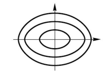
The variation of the variables p 𝑝 p q 𝑞 q y 𝑦 y x 𝑥 x
p ˙ = − ∂ E ∂ q , q ˙ = ∂ E ∂ p , y ˙ = − ε ∂ E ∂ x , x ˙ = ε ∂ E ∂ y . formulae-sequence ˙ 𝑝 𝐸 𝑞 formulae-sequence ˙ 𝑞 𝐸 𝑝 formulae-sequence ˙ 𝑦 𝜀 𝐸 𝑥 ˙ 𝑥 𝜀 𝐸 𝑦 \dot{p}=-\frac{\partial E}{\partial q},\quad\dot{q}=\frac{\partial E}{\partial p},\quad\dot{y}=-\varepsilon\frac{\partial E}{\partial x},\quad\dot{x}=\varepsilon\frac{\partial E}{\partial y}.
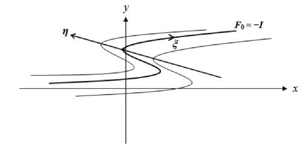
The variables p 𝑝 p q 𝑞 q y 𝑦 y x 𝑥 x y = const 𝑦 const y=\mathrm{const} x = const 𝑥 const x=\mathrm{const} y , x = const 𝑦 𝑥
const y,x=\mathrm{const} [1 ] :
Figure 1:
Here the frequency of motion is non-zero. So we can introduce action-angle variables
I = I ( p , q , y , x ) , φ = φ ( p , q , y , x ) mod 2 π formulae-sequence 𝐼 𝐼 𝑝 𝑞 𝑦 𝑥 𝜑 modulo 𝜑 𝑝 𝑞 𝑦 𝑥 2 𝜋 I=I(p,q,y,x),\quad\varphi=\varphi(p,q,y,x)\mod{2\pi}
The action I 𝐼 I 2 π 2 𝜋 2\pi H 0 ( I , y , x ) subscript 𝐻 0 𝐼 𝑦 𝑥 H_{0}(I,y,x) E 𝐸 E I 𝐼 I y 𝑦 y x 𝑥 x I = const 𝐼 const I=\mathrm{const} y 𝑦 y x 𝑥 x H 0 ( I , y , x ) subscript 𝐻 0 𝐼 𝑦 𝑥 H_{0}(I,y,x)
E ( p , q , y , x ) ≡ H 0 ( I , y , x ) , 𝐸 𝑝 𝑞 𝑦 𝑥 subscript 𝐻 0 𝐼 𝑦 𝑥 E(p,q,y,x)\equiv H_{0}(I,y,x),
y ˙ = − ε ∂ H 0 ( I , y , x ) ∂ x , x ˙ = ε ∂ H 0 ( I , y , x ) ∂ y . formulae-sequence ˙ 𝑦 𝜀 subscript 𝐻 0 𝐼 𝑦 𝑥 𝑥 ˙ 𝑥 𝜀 subscript 𝐻 0 𝐼 𝑦 𝑥 𝑦 \dot{y}=-\varepsilon\frac{\partial H_{0}(I,y,x)}{\partial x},\quad\dot{x}=\varepsilon\frac{\partial H_{0}(I,y,x)}{\partial y}.
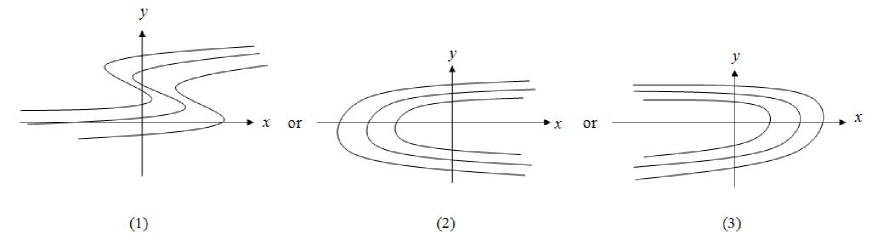
We will assume that in the phase portrait of this system there is a domain in which along trajectories | x | → ∞ → 𝑥 |x|\to\infty y → const → 𝑦 const y\to\mathrm{const} t → ± ∞ → 𝑡 plus-or-minus t\to\pm\infty
Figure 2:
We consider the case when the adiabatic invariant of the action I 𝐼 I I ± subscript 𝐼 plus-or-minus I_{\pm} t → ± ∞ → 𝑡 plus-or-minus t\to\pm\infty Δ I = I + − I − Δ 𝐼 subscript 𝐼 subscript 𝐼 \Delta I=I_{+}-I_{-}
If this system is analytic, the value of Δ I Δ 𝐼 \Delta I [1 ] :
Δ I = O ( e − γ ε ) , γ = const > 0 . formulae-sequence Δ 𝐼 𝑂 superscript e 𝛾 𝜀 𝛾 const 0 \Delta I=O(\mathrm{e}^{-\frac{\gamma}{\varepsilon}}),\quad\gamma=\mathrm{const}>0.
The goal of this paper is to find an estimate of constant γ 𝛾 \gamma
2 Reduction to a standard form
For the original Hamiltonian E ( p , q , y , x ) 𝐸 𝑝 𝑞 𝑦 𝑥 E(p,q,y,x) y , x = const 𝑦 𝑥
const y,x=\mathrm{const} q 𝑞 q p 𝑝 p T 𝑇 T ω 𝜔 \omega S ( I , q , y , x ) 𝑆 𝐼 𝑞 𝑦 𝑥 S(I,q,y,x) ( p , q ) ↦ ( I , φ ) maps-to 𝑝 𝑞 𝐼 𝜑 (p,q)\mapsto(I,\varphi) [3 ] :
φ = ∂ S ( I , q , y , x ) ∂ I , p = ∂ S ( I , q , y , x ) ∂ q . formulae-sequence 𝜑 𝑆 𝐼 𝑞 𝑦 𝑥 𝐼 𝑝 𝑆 𝐼 𝑞 𝑦 𝑥 𝑞 \varphi=\frac{\partial S(I,q,y,x)}{\partial I},\quad p=\frac{\partial S(I,q,y,x)}{\partial q}.
For a fixed trajectory E ( p , q , y , x ) = h = H 0 ( I , y , x ) 𝐸 𝑝 𝑞 𝑦 𝑥 ℎ subscript 𝐻 0 𝐼 𝑦 𝑥 E(p,q,y,x)=h=H_{0}(I,y,x) h ℎ h p 𝑝 p
p = P ( h , q , y , x ) 𝑝 𝑃 ℎ 𝑞 𝑦 𝑥 p=P(h,q,y,x)
if ∂ E ∂ p ≠ 0 𝐸 𝑝 0 \displaystyle\frac{\partial E}{\partial p}\neq 0 [3 ] :
S ( I , q , y , x ) = ∫ q 0 q P ( h ( I , y , x ) , q 1 , y , x ) d q 1 , 𝑆 𝐼 𝑞 𝑦 𝑥 superscript subscript subscript 𝑞 0 𝑞 𝑃 ℎ 𝐼 𝑦 𝑥 subscript 𝑞 1 𝑦 𝑥 differential-d subscript 𝑞 1 S(I,q,y,x)=\int\limits_{q_{0}}^{q}P(h(I,y,x),q_{1},y,x)\,\mathrm{d}q_{1},
where the constant q 0 subscript 𝑞 0 q_{0} q 1 subscript 𝑞 1 q_{1}
Lemma 2.1 .
(see, e.g. [4 ] )
∂ S ∂ x = ∫ 0 t ( ⟨ ∂ E ∂ x ⟩ − ∂ E ∂ x ) d t 1 , 𝑆 𝑥 superscript subscript 0 𝑡 delimited-⟨⟩ 𝐸 𝑥 𝐸 𝑥 differential-d subscript 𝑡 1 \frac{\partial S}{\partial x}=\int\limits_{0}^{t}\left(\left<\frac{\partial E}{\partial x}\right>-\frac{\partial E}{\partial x}\right)\,\mathrm{d}t_{1},
∂ S ∂ y = ∫ 0 t ( ⟨ ∂ E ∂ y ⟩ − ∂ E ∂ y ) d t 1 𝑆 𝑦 superscript subscript 0 𝑡 delimited-⟨⟩ 𝐸 𝑦 𝐸 𝑦 differential-d subscript 𝑡 1 \frac{\partial S}{\partial y}=\int\limits_{0}^{t}\left(\left<\frac{\partial E}{\partial y}\right>-\frac{\partial E}{\partial y}\right)\,\mathrm{d}t_{1}
where
⟨ ∂ E ∂ x ⟩ = 1 T ∮ ∂ E ∂ x d t 1 , ⟨ ∂ E ∂ y ⟩ = 1 T ∮ ∂ E ∂ y d t 1 . formulae-sequence delimited-⟨⟩ 𝐸 𝑥 1 𝑇 contour-integral 𝐸 𝑥 differential-d subscript 𝑡 1 delimited-⟨⟩ 𝐸 𝑦 1 𝑇 contour-integral 𝐸 𝑦 differential-d subscript 𝑡 1 \left<\frac{\partial E}{\partial x}\right>=\frac{1}{T}\oint\frac{\partial E}{\partial x}\,\mathrm{d}t_{1},\quad\left<\frac{\partial E}{\partial y}\right>=\frac{1}{T}\oint\frac{\partial E}{\partial y}\,\mathrm{d}t_{1}.
Now consider another canonical transformation ( p , q , y , x ) ↦ ( I ¯ , φ ¯ , y ¯ , x ¯ ) maps-to 𝑝 𝑞 𝑦 𝑥 ¯ 𝐼 ¯ 𝜑 ¯ 𝑦 ¯ 𝑥 (p,q,y,x)\mapsto(\bar{I},\bar{\varphi},\bar{y},\bar{x}) ε − 1 y ¯ x + S ( I ¯ , q , y ¯ , x ) superscript 𝜀 1 ¯ 𝑦 𝑥 𝑆 ¯ 𝐼 𝑞 ¯ 𝑦 𝑥 \varepsilon^{-1}\bar{y}x+S(\bar{I},q,\bar{y},x) ( p , q ) 𝑝 𝑞 (p,q) ( y , ε − 1 x ) 𝑦 superscript 𝜀 1 𝑥 (y,\varepsilon^{-1}x) ( I ¯ , φ ¯ ) ¯ 𝐼 ¯ 𝜑 (\bar{I},\bar{\varphi}) ( y ¯ , ε − 1 x ¯ ) ¯ 𝑦 superscript 𝜀 1 ¯ 𝑥 (\bar{y},\varepsilon^{-1}\bar{x})
Lemma 2.2 .
(see, e.g. [1 ] )
y = y ¯ + O ( ε ) , x = x ¯ + O ( ε ) , I = I ¯ + O ( ε ) , φ = φ ¯ + O ( ε ) formulae-sequence 𝑦 ¯ 𝑦 𝑂 𝜀 formulae-sequence 𝑥 ¯ 𝑥 𝑂 𝜀 formulae-sequence 𝐼 ¯ 𝐼 𝑂 𝜀 𝜑 ¯ 𝜑 𝑂 𝜀 y=\bar{y}+O(\varepsilon),\ x=\bar{x}+O(\varepsilon),\ I=\bar{I}+O(\varepsilon),\ \varphi=\bar{\varphi}+O(\varepsilon)
and new Hamiltonian is
H = H 0 ( I ¯ , y ¯ , x ¯ ) + ε H 1 ( I ¯ , φ ¯ , y ¯ , x ¯ , ε ) . 𝐻 subscript 𝐻 0 ¯ 𝐼 ¯ 𝑦 ¯ 𝑥 𝜀 subscript 𝐻 1 ¯ 𝐼 ¯ 𝜑 ¯ 𝑦 ¯ 𝑥 𝜀 H=H_{0}(\bar{I},\bar{y},\bar{x})+\varepsilon H_{1}(\bar{I},\bar{\varphi},\bar{y},\bar{x},\varepsilon).
We will consider the case that there exist limiting values of action variables I 𝐼 I I ¯ ¯ 𝐼 \bar{I} I 𝐼 I I ¯ ¯ 𝐼 \bar{I}
So far we have got a new Hamiltonian
H ( I ¯ , φ ¯ , y ¯ , x ¯ , ε ) = H 0 ( I ¯ , y ¯ , x ¯ ) + ε H 1 ( I ¯ , φ ¯ , y ¯ , x ¯ , ε ) . 𝐻 ¯ 𝐼 ¯ 𝜑 ¯ 𝑦 ¯ 𝑥 𝜀 subscript 𝐻 0 ¯ 𝐼 ¯ 𝑦 ¯ 𝑥 𝜀 subscript 𝐻 1 ¯ 𝐼 ¯ 𝜑 ¯ 𝑦 ¯ 𝑥 𝜀 H(\bar{I},\bar{\varphi},\bar{y},\bar{x},\varepsilon)=H_{0}(\bar{I},\bar{y},\bar{x})+\varepsilon H_{1}(\bar{I},\bar{\varphi},\bar{y},\bar{x},\varepsilon).
For simplicity, omitting the bar symbols and dependence on ε 𝜀 \varepsilon
H ( I , φ , y , x ) = H 0 ( I , y , x ) + ε H 1 ( I , φ , y , x ) 𝐻 𝐼 𝜑 𝑦 𝑥 subscript 𝐻 0 𝐼 𝑦 𝑥 𝜀 subscript 𝐻 1 𝐼 𝜑 𝑦 𝑥 H(I,\varphi,y,x)=H_{0}(I,y,x)+\varepsilon H_{1}(I,\varphi,y,x)
which has motion
I ˙ = − ε ∂ H 1 ∂ φ , φ ˙ = ∂ H 0 ∂ I + ε ∂ H 1 ∂ I , formulae-sequence ˙ 𝐼 𝜀 subscript 𝐻 1 𝜑 ˙ 𝜑 subscript 𝐻 0 𝐼 𝜀 subscript 𝐻 1 𝐼 \displaystyle\dot{I}=-\varepsilon\frac{\partial H_{1}}{\partial\varphi},\quad\dot{\varphi}=\frac{\partial H_{0}}{\partial I}+\varepsilon\frac{\partial H_{1}}{\partial I},
y ˙ = − ε ( ∂ H 0 ∂ x + ε ∂ H 1 ∂ x ) , x ˙ = ε ( ∂ H 0 ∂ y + ε ∂ H 1 ∂ y ) . formulae-sequence ˙ 𝑦 𝜀 subscript 𝐻 0 𝑥 𝜀 subscript 𝐻 1 𝑥 ˙ 𝑥 𝜀 subscript 𝐻 0 𝑦 𝜀 subscript 𝐻 1 𝑦 \displaystyle\dot{y}=-\varepsilon\left(\frac{\partial H_{0}}{\partial x}+\varepsilon\frac{\partial H_{1}}{\partial x}\right),\quad\dot{x}=\varepsilon\left(\frac{\partial H_{0}}{\partial y}+\varepsilon\frac{\partial H_{1}}{\partial y}\right).
3 Statement of the problem
It is assumed, that in adiabatic approximation, | x | → ∞ → 𝑥 |x|\to\infty y → const → 𝑦 const y\to\mathrm{const} t → ± ∞ → 𝑡 plus-or-minus t\to\pm\infty x 𝑥 x y 𝑦 y p 𝑝 p q 𝑞 q
∂ E ( p , q , x , y ) ∂ x → 0 , as t → ± ∞ . formulae-sequence → 𝐸 𝑝 𝑞 𝑥 𝑦 𝑥 0 → as 𝑡 plus-or-minus \frac{\partial E(p,q,x,y)}{\partial x}\to 0,\quad\text{as\ }t\to\pm\infty.
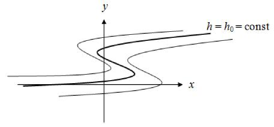
For definiteness we will consider the case when the trajectories in adiabatic approximation have the form shown in Figure 2(1). Result will be valid for the other two cases of Figure 2.
The function
ω 0 ( I , y , x ) = ∂ H 0 ( I , y , x ) ∂ I subscript 𝜔 0 𝐼 𝑦 𝑥 subscript 𝐻 0 𝐼 𝑦 𝑥 𝐼 \omega_{0}(I,y,x)=\displaystyle\frac{\partial H_{0}(I,y,x)}{\partial I}
is the frequency of unperturbed motion.
Let us assume that the following conditions are fulfilled.
Assumption 1 ∘ superscript 1 1^{\circ}
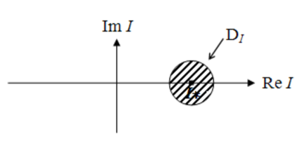
The functions H 0 subscript 𝐻 0 H_{0} H 1 subscript 𝐻 1 H_{1} D = D I × D φ × D x y 𝐷 subscript 𝐷 𝐼 subscript 𝐷 𝜑 subscript 𝐷 𝑥 𝑦 D=D_{I}\times D_{\varphi}\times D_{xy} D I subscript 𝐷 𝐼 D_{I} I ∗ subscript 𝐼 I_{*}
Figure 3:
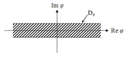
D φ subscript 𝐷 𝜑 D_{\varphi}
Figure 4:
and D x y subscript 𝐷 𝑥 𝑦 D_{xy} ℂ 2 superscript ℂ 2 \mathbb{C}^{2} ω 0 ( I , y , x ) subscript 𝜔 0 𝐼 𝑦 𝑥 \omega_{0}(I,y,x) D 𝐷 D | ω 0 | > const subscript 𝜔 0 const \left|\omega_{0}\right|>\mathrm{const} H 0 ( I , y , x ) subscript 𝐻 0 𝐼 𝑦 𝑥 H_{0}(I,y,x)
| ∂ H 0 ∂ I | < const , | ∂ H 0 ∂ y | < const , | ∂ H 0 ∂ x | < const , ( ∂ H 0 ∂ y ) 2 + ( ∂ H 0 ∂ x ) 2 > const . formulae-sequence subscript 𝐻 0 𝐼 const formulae-sequence subscript 𝐻 0 𝑦 const formulae-sequence subscript 𝐻 0 𝑥 const superscript subscript 𝐻 0 𝑦 2 superscript subscript 𝐻 0 𝑥 2 const \left|\frac{\partial H_{0}}{\partial I}\right|<\mathrm{const},\quad\left|\frac{\partial H_{0}}{\partial y}\right|<\mathrm{const},\quad\left|\frac{\partial H_{0}}{\partial x}\right|<\mathrm{const},\quad\left(\frac{\partial H_{0}}{\partial y}\right)^{2}+\left(\frac{\partial H_{0}}{\partial x}\right)^{2}>\mathrm{const}.
Now let us consider approximate Hamiltonian H 0 ( I , y , x ) subscript 𝐻 0 𝐼 𝑦 𝑥 H_{0}(I,y,x)
y ˙ = − ε ∂ H 0 ∂ x , x ˙ = ε ∂ H 0 ∂ y . formulae-sequence ˙ 𝑦 𝜀 subscript 𝐻 0 𝑥 ˙ 𝑥 𝜀 subscript 𝐻 0 𝑦 \dot{y}=-\varepsilon\frac{\partial H_{0}}{\partial x},\quad\dot{x}=\varepsilon\frac{\partial H_{0}}{\partial y}.
For a fixed I 0 subscript 𝐼 0 I_{0} H 0 ( I 0 , y , x ) = h = const subscript 𝐻 0 subscript 𝐼 0 𝑦 𝑥 ℎ const H_{0}(I_{0},y,x)=h=\mathrm{const} H 0 = const subscript 𝐻 0 const H_{0}=\mathrm{const}
Figure 5:
Introduce the slow time
τ = ε t . 𝜏 𝜀 𝑡 \tau=\varepsilon t.
The differential equations of motion are
d y d τ = − ∂ H 0 ∂ x , d x d τ = ∂ H 0 ∂ y . formulae-sequence d 𝑦 d 𝜏 subscript 𝐻 0 𝑥 d 𝑥 d 𝜏 subscript 𝐻 0 𝑦 \frac{\mathrm{d}y}{\mathrm{d}\tau}=-\frac{\partial H_{0}}{\partial x},\quad\frac{\mathrm{d}x}{\mathrm{d}\tau}=\frac{\partial H_{0}}{\partial y}.
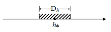
Take h = h 0 ℎ subscript ℎ 0 h=h_{0} h 0 subscript ℎ 0 h_{0} D h subscript 𝐷 ℎ D_{h} h ∗ subscript ℎ h_{*} h ∗ subscript ℎ h_{*}
Figure 6:
We can find the solution for describing the motion for approximate Hamiltonian H 0 subscript 𝐻 0 H_{0} H 0 ( I 0 , y , x ) = h 0 subscript 𝐻 0 subscript 𝐼 0 𝑦 𝑥 subscript ℎ 0 H_{0}(I_{0},y,x)=h_{0}
{ y = Y ( τ , I 0 , h 0 ) x = X ( τ , I 0 , h 0 ) I 0 ∈ D I , h 0 ∈ D h . formulae-sequence cases 𝑦 𝑌 𝜏 subscript 𝐼 0 subscript ℎ 0 missing-subexpression missing-subexpression 𝑥 𝑋 𝜏 subscript 𝐼 0 subscript ℎ 0 missing-subexpression missing-subexpression subscript 𝐼 0
subscript 𝐷 𝐼 subscript ℎ 0 subscript 𝐷 ℎ \left\{\begin{array}[]{ccc}y=Y(\tau,I_{0},h_{0})\\
x=X(\tau,I_{0},h_{0})\end{array}\right.\qquad I_{0}\in D_{I},\quad h_{0}\in D_{h}.
From now on we omit the dependence on h 0 subscript ℎ 0 h_{0}
Assumption 2 ∘ superscript 2 2^{\circ}
The solutions Y ( τ , I 0 ) 𝑌 𝜏 subscript 𝐼 0 Y(\tau,I_{0}) X ( τ , I 0 ) 𝑋 𝜏 subscript 𝐼 0 X(\tau,I_{0})
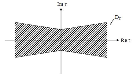
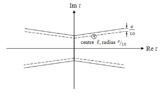
D τ = { τ : | Im τ | < σ + δ | Re τ | } . subscript 𝐷 𝜏 conditional-set 𝜏 Im 𝜏 𝜎 𝛿 Re 𝜏 D_{\tau}=\{\tau\colon|\mathrm{Im}\ \tau|<\sigma+\delta|\mathrm{Re}\ \tau|\}.
Figure 7:
We suppose that for any initial point, the solution tends to infinity as time tends to infinity, i.e.
lim Re τ → ± ∞ | X ( τ , I 0 ) | = ∞ . subscript → Re 𝜏 plus-or-minus 𝑋 𝜏 subscript 𝐼 0 \lim\limits_{\mathrm{Re}\,\tau\to\pm\infty}\big{|}X(\tau,I_{0})\big{|}=\infty.
H 0 ( I , y , x ) subscript 𝐻 0 𝐼 𝑦 𝑥 H_{0}(I,y,x)
lim Re τ → ± ∞ ∂ H 0 ( I , Y ( τ , I 0 ) , X ( τ , I 0 ) ) ∂ x = 0 . subscript → Re 𝜏 plus-or-minus subscript 𝐻 0 𝐼 𝑌 𝜏 subscript 𝐼 0 𝑋 𝜏 subscript 𝐼 0 𝑥 0 \lim\limits_{\mathrm{Re}\,\tau\to\pm\infty}\frac{\partial H_{0}(I,Y(\tau,I_{0}),X(\tau,I_{0}))}{\partial x}=0.
H 1 ( I , φ , y , x ) subscript 𝐻 1 𝐼 𝜑 𝑦 𝑥 H_{1}(I,\varphi,y,x)
| H 1 ( I , φ , Y ( τ , I 0 ) , X ( τ , I 0 ) ) | < c 1 + | ∫ 0 τ ω 0 ( I 0 , Y ( τ 1 , I 0 ) , X ( τ 1 , I 0 ) ) d τ 1 | 2 + ν . subscript 𝐻 1 𝐼 𝜑 𝑌 𝜏 subscript 𝐼 0 𝑋 𝜏 subscript 𝐼 0 𝑐 1 superscript superscript subscript 0 𝜏 subscript 𝜔 0 subscript 𝐼 0 𝑌 subscript 𝜏 1 subscript 𝐼 0 𝑋 subscript 𝜏 1 subscript 𝐼 0 differential-d subscript 𝜏 1 2 𝜈 |H_{1}(I,\varphi,Y(\tau,I_{0}),X(\tau,I_{0}))|<\frac{c}{1+\left|\int\limits_{0}^{\tau}\omega_{0}(I_{0},Y(\tau_{1},I_{0}),X(\tau_{1},I_{0}))\,\mathrm{d}\tau_{1}\right|^{2+\nu}}.
ω 0 ( I , y , x ) subscript 𝜔 0 𝐼 𝑦 𝑥 \omega_{0}(I,y,x)
Im ω 0 ( I 0 , Y ( τ , I 0 ) , X ( τ , I 0 ) ) ⇉ 0 , as Re τ → ± ∞ , Im I 0 → 0 . formulae-sequence ⇉ Im subscript 𝜔 0 subscript 𝐼 0 𝑌 𝜏 subscript 𝐼 0 𝑋 𝜏 subscript 𝐼 0 0 formulae-sequence → as Re 𝜏 plus-or-minus → Im subscript 𝐼 0 0 \mathrm{Im}\ \omega_{0}(I_{0},Y(\tau,I_{0}),X(\tau,I_{0}))\rightrightarrows 0,\quad\mathrm{as}\ \mathrm{Re}\;\tau\to\pm\infty,\ \mathrm{Im}\;I_{0}\to 0.
Here σ 𝜎 \sigma δ 𝛿 \delta c 𝑐 c ν 𝜈 \nu
Lemma 3.1 .
For I ∈ D ~ I = D I − δ I 𝐼 subscript ~ 𝐷 𝐼 subscript 𝐷 𝐼 subscript 𝛿 𝐼 I\in\widetilde{D}_{I}=D_{I}-\delta_{I} φ ∈ D ~ φ = D φ − δ φ 𝜑 subscript ~ 𝐷 𝜑 subscript 𝐷 𝜑 subscript 𝛿 𝜑 \varphi\in\widetilde{D}_{\varphi}=D_{\varphi}-\delta_{\varphi} τ ∈ D ~ τ = { τ : | Im τ | < σ − δ τ + δ | Re τ | } 𝜏 subscript ~ 𝐷 𝜏 conditional-set 𝜏 Im 𝜏 𝜎 subscript 𝛿 𝜏 𝛿 Re 𝜏 \tau\in\widetilde{D}_{\tau}=\{\tau\colon|\mathrm{Im}\ \tau|<\sigma-\delta_{\tau}+\delta|\mathrm{Re}\ \tau|\}
| ∂ H 1 ( I , φ , Y ( τ , I 0 ) , X ( τ , I 0 ) ) ∂ I | < const 1 + | ∫ 0 τ ω 0 ( I 0 , Y ( τ 1 , I 0 ) , X ( τ 1 , I 0 ) ) d τ 1 | 2 + ν , subscript 𝐻 1 𝐼 𝜑 𝑌 𝜏 subscript 𝐼 0 𝑋 𝜏 subscript 𝐼 0 𝐼 const 1 superscript superscript subscript 0 𝜏 subscript 𝜔 0 subscript 𝐼 0 𝑌 subscript 𝜏 1 subscript 𝐼 0 𝑋 subscript 𝜏 1 subscript 𝐼 0 differential-d subscript 𝜏 1 2 𝜈 \displaystyle\left|\frac{\partial H_{1}(I,\varphi,Y(\tau,I_{0}),X(\tau,I_{0}))}{\partial I}\right|<\frac{\mathrm{const}}{1+\left|\int\limits_{0}^{\tau}\omega_{0}(I_{0},Y(\tau_{1},I_{0}),X(\tau_{1},I_{0}))\,\mathrm{d}\tau_{1}\right|^{2+\nu}},
| ∂ H 1 ( I , φ , Y ( τ , I 0 ) , X ( τ , I 0 ) ) ∂ φ | < const 1 + | ∫ 0 τ ω 0 ( I 0 , Y ( τ 1 , I 0 ) , X ( τ 1 , I 0 ) ) d τ 1 | 2 + ν , subscript 𝐻 1 𝐼 𝜑 𝑌 𝜏 subscript 𝐼 0 𝑋 𝜏 subscript 𝐼 0 𝜑 const 1 superscript superscript subscript 0 𝜏 subscript 𝜔 0 subscript 𝐼 0 𝑌 subscript 𝜏 1 subscript 𝐼 0 𝑋 subscript 𝜏 1 subscript 𝐼 0 differential-d subscript 𝜏 1 2 𝜈 \displaystyle\left|\frac{\partial H_{1}(I,\varphi,Y(\tau,I_{0}),X(\tau,I_{0}))}{\partial\varphi}\right|<\frac{\mathrm{const}}{1+\left|\int\limits_{0}^{\tau}\omega_{0}(I_{0},Y(\tau_{1},I_{0}),X(\tau_{1},I_{0}))\,\mathrm{d}\tau_{1}\right|^{2+\nu}},
| ∂ H 1 ( I , φ , Y ( τ , I 0 ) , X ( τ , I 0 ) ) ∂ τ | < const 1 + | ∫ 0 τ ω 0 ( I 0 , Y ( τ 1 , I 0 ) , X ( τ 1 , I 0 ) ) d τ 1 | 2 + ν , subscript 𝐻 1 𝐼 𝜑 𝑌 𝜏 subscript 𝐼 0 𝑋 𝜏 subscript 𝐼 0 𝜏 const 1 superscript superscript subscript 0 𝜏 subscript 𝜔 0 subscript 𝐼 0 𝑌 subscript 𝜏 1 subscript 𝐼 0 𝑋 subscript 𝜏 1 subscript 𝐼 0 differential-d subscript 𝜏 1 2 𝜈 \displaystyle\left|\frac{\partial H_{1}(I,\varphi,Y(\tau,I_{0}),X(\tau,I_{0}))}{\partial\tau}\right|<\frac{\mathrm{const}}{1+\left|\int\limits_{0}^{\tau}\omega_{0}(I_{0},Y(\tau_{1},I_{0}),X(\tau_{1},I_{0}))\,\mathrm{d}\tau_{1}\right|^{2+\nu}},
where δ I subscript 𝛿 𝐼 \delta_{I} δ φ subscript 𝛿 𝜑 \delta_{\varphi} δ τ subscript 𝛿 𝜏 \delta_{\tau}
Proof.
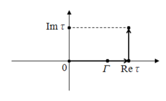
Im ω 0 ( I 0 , Y ( τ , I 0 ) , X ( τ , I 0 ) ) ⇉ 0 , as Re τ → ± ∞ , Im I 0 → 0 formulae-sequence ⇉ Im subscript 𝜔 0 subscript 𝐼 0 𝑌 𝜏 subscript 𝐼 0 𝑋 𝜏 subscript 𝐼 0 0 formulae-sequence → as Re 𝜏 plus-or-minus → Im subscript 𝐼 0 0 \mathrm{Im}\ \omega_{0}(I_{0},Y(\tau,I_{0}),X(\tau,I_{0}))\rightrightarrows 0,\quad\mathrm{as}\ \mathrm{Re}\;\tau\to\pm\infty,\ \mathrm{Im}\;I_{0}\to 0 ∀ ρ > 0 , ∃ Σ > 0 , Γ > 0 , such that if | Im I 0 | < Σ , | Re τ | > Γ , then formulae-sequence for-all 𝜌 0 formulae-sequence Σ 0 formulae-sequence Γ 0 formulae-sequence such that if Im subscript 𝐼 0 Σ Re 𝜏 Γ then
\forall\,\rho>0,\ \exists\,\Sigma>0,\ \Gamma>0,\ \mathrm{such\ that}\ \mathrm{if}\ |\mathrm{Im}\;I_{0}|<\Sigma,\ |\mathrm{Re}\;\tau|>\Gamma,\ \mathrm{then}
| Im ω 0 | < ρ . Im subscript 𝜔 0 𝜌 |\mathrm{Im}\ \omega_{0}|<\rho.
Since we know that | ω 0 | > c 1 = const subscript 𝜔 0 subscript 𝑐 1 const |\omega_{0}|>c_{1}=\mathrm{const} | Im ω 0 | < c 1 10 Im subscript 𝜔 0 subscript 𝑐 1 10 |\mathrm{Im}\ \omega_{0}|<\displaystyle\frac{c_{1}}{10} | Im I 0 | < Σ Im subscript 𝐼 0 Σ |\mathrm{Im}\;I_{0}|<\Sigma | Re τ | > Γ Re 𝜏 Γ |\mathrm{Re}\;\tau|>\Gamma
| Re ω 0 | > 9 10 c 1 . Re subscript 𝜔 0 9 10 subscript 𝑐 1 |\mathrm{Re}\ \omega_{0}|>\displaystyle\frac{9}{10}c_{1}.
Let τ = λ + i μ 𝜏 𝜆 i 𝜇 \tau=\lambda+\mathrm{i}\mu | ∫ 0 τ ω 0 ( I 0 , Y ( τ 1 , I 0 ) , X ( τ 1 , I 0 ) ) d τ 1 | superscript subscript 0 𝜏 subscript 𝜔 0 subscript 𝐼 0 𝑌 subscript 𝜏 1 subscript 𝐼 0 𝑋 subscript 𝜏 1 subscript 𝐼 0 differential-d subscript 𝜏 1 \left|\int\limits_{0}^{\tau}\omega_{0}(I_{0},Y(\tau_{1},I_{0}),X(\tau_{1},I_{0}))\,\mathrm{d}\tau_{1}\right|
For | Re τ | > max { Γ , 2 ( 9 10 c 1 − ρ ) − 1 ( 9 10 c 1 + ρ + a + b ) Γ } Re 𝜏 Γ 2 superscript 9 10 subscript 𝑐 1 𝜌 1 9 10 subscript 𝑐 1 𝜌 𝑎 𝑏 Γ |\mathrm{Re}\;\tau|>\max\Big{\{}\Gamma,\ 2\Big{(}\dfrac{9}{10}c_{1}-\rho\Big{)}^{-1}\Big{(}\dfrac{9}{10}c_{1}+\rho+a+b\Big{)}\Gamma\Big{\}} a 𝑎 a b 𝑏 b
∫ 0 Γ | Re ω 0 | d λ ≤ a ⋅ Γ , ∫ 0 Γ | Im ω 0 | d λ ≤ b ⋅ Γ , formulae-sequence superscript subscript 0 Γ Re subscript 𝜔 0 differential-d 𝜆 ⋅ 𝑎 Γ superscript subscript 0 Γ Im subscript 𝜔 0 differential-d 𝜆 ⋅ 𝑏 Γ \int\limits_{0}^{\Gamma}|\mathrm{Re}\;\omega_{0}|\,\mathrm{d}\lambda\leq a\cdot\Gamma,\quad\int\limits_{0}^{\Gamma}|\mathrm{Im}\;\omega_{0}|\,\mathrm{d}\lambda\leq b\cdot\Gamma,
Figure 8:
we have
| ∫ 0 τ ω 0 d τ 1 | superscript subscript 0 𝜏 subscript 𝜔 0 differential-d subscript 𝜏 1 \displaystyle\left|\int\limits_{0}^{\tau}\omega_{0}\,\mathrm{d}\tau_{1}\right| = \displaystyle= | ∫ 0 Re τ ω 0 d τ 1 + ∫ Re τ τ ω 0 d τ 1 | superscript subscript 0 Re 𝜏 subscript 𝜔 0 differential-d subscript 𝜏 1 superscript subscript Re 𝜏 𝜏 subscript 𝜔 0 differential-d subscript 𝜏 1 \displaystyle\left|\int\limits_{0}^{\mathrm{Re}\,\tau}\omega_{0}\,\mathrm{d}\tau_{1}+\int\limits_{\mathrm{Re}\,\tau}^{\tau}\omega_{0}\,\mathrm{d}\tau_{1}\right|
= \displaystyle= | ∫ 0 Re τ ω 0 d ( λ + i μ ) + ∫ Re τ τ ω 0 d ( λ + i μ ) | superscript subscript 0 Re 𝜏 subscript 𝜔 0 d 𝜆 i 𝜇 superscript subscript Re 𝜏 𝜏 subscript 𝜔 0 d 𝜆 i 𝜇 \displaystyle\left|\int\limits_{0}^{\mathrm{Re}\,\tau}\omega_{0}\,\mathrm{d}(\lambda+\mathrm{i}\mu)+\int\limits_{\mathrm{Re}\,\tau}^{\tau}\omega_{0}\,\mathrm{d}(\lambda+\mathrm{i}\mu)\right|
= \displaystyle= | ∫ 0 Re τ ω 0 d λ + ∫ Re τ τ ω 0 d ( i μ ) | superscript subscript 0 Re 𝜏 subscript 𝜔 0 differential-d 𝜆 superscript subscript Re 𝜏 𝜏 subscript 𝜔 0 d i 𝜇 \displaystyle\left|\int\limits_{0}^{\mathrm{Re}\,\tau}\omega_{0}\,\mathrm{d}\lambda+\int\limits_{\mathrm{Re}\,\tau}^{\tau}\omega_{0}\,\mathrm{d}(\mathrm{i}\mu)\right|
= \displaystyle= | ∫ 0 Re τ Re ω 0 d λ + ∫ 0 Re τ i Im ω 0 d λ + ∫ Re τ τ Re ω 0 d ( i μ ) + ∫ Re τ τ i Im ω 0 d ( i μ ) | superscript subscript 0 Re 𝜏 Re subscript 𝜔 0 differential-d 𝜆 superscript subscript 0 Re 𝜏 i Im subscript 𝜔 0 differential-d 𝜆 superscript subscript Re 𝜏 𝜏 Re subscript 𝜔 0 d i 𝜇 superscript subscript Re 𝜏 𝜏 i Im subscript 𝜔 0 d i 𝜇 \displaystyle\left|\int\limits_{0}^{\mathrm{Re}\,\tau}\mathrm{Re}\;\omega_{0}\,\mathrm{d}\lambda+\int\limits_{0}^{\mathrm{Re}\,\tau}\mathrm{i}\;\mathrm{Im}\;\omega_{0}\,\mathrm{d}\lambda+\int\limits_{\mathrm{Re}\,\tau}^{\tau}\mathrm{Re}\;\omega_{0}\,\mathrm{d}(\mathrm{i}\mu)+\int\limits_{\mathrm{Re}\,\tau}^{\tau}\mathrm{i}\;\mathrm{Im}\;\omega_{0}\,\mathrm{d}(\mathrm{i}\mu)\right|
= \displaystyle= | ∫ 0 Γ Re ω 0 d λ + ∫ Γ Re τ Re ω 0 d λ + ∫ 0 Γ i Im ω 0 d λ + ∫ Γ Re τ i Im ω 0 d λ \displaystyle\left|\int\limits_{0}^{\Gamma}\mathrm{Re}\;\omega_{0}\,\mathrm{d}\lambda+\int\limits_{\Gamma}^{\mathrm{Re}\,\tau}\mathrm{Re}\;\omega_{0}\,\mathrm{d}\lambda+\int\limits_{0}^{\Gamma}\mathrm{i}\;\mathrm{Im}\;\omega_{0}\,\mathrm{d}\lambda+\int\limits_{\Gamma}^{\mathrm{Re}\,\tau}\mathrm{i}\;\mathrm{Im}\;\omega_{0}\,\mathrm{d}\lambda\right.
+ ∫ Re τ τ Re ω 0 d ( i μ ) + ∫ Re τ τ i Im ω 0 d ( i μ ) | \displaystyle\left.+\int\limits_{\mathrm{Re}\,\tau}^{\tau}\mathrm{Re}\;\omega_{0}\,\mathrm{d}(\mathrm{i}\mu)+\int\limits_{\mathrm{Re}\,\tau}^{\tau}\mathrm{i}\;\mathrm{Im}\;\omega_{0}\,\mathrm{d}(\mathrm{i}\mu)\right|
≥ \displaystyle\geq | | ∫ Γ Re τ Re ω 0 d λ + ∫ Re τ τ Re ω 0 d ( i μ ) | − | ∫ Γ Re τ | Im ω 0 | d λ + ∫ Re τ τ | Im ω 0 | d ( i μ ) superscript subscript Γ Re 𝜏 Re subscript 𝜔 0 differential-d 𝜆 superscript subscript Re 𝜏 𝜏 Re subscript 𝜔 0 d i 𝜇 superscript subscript Γ Re 𝜏 Im subscript 𝜔 0 d 𝜆 superscript subscript Re 𝜏 𝜏 Im subscript 𝜔 0 d i 𝜇 \displaystyle\left|\left|\int\limits_{\Gamma}^{\mathrm{Re}\,\tau}\mathrm{Re}\;\omega_{0}\,\mathrm{d}\lambda+\int\limits_{\mathrm{Re}\,\tau}^{\tau}\mathrm{Re}\;\omega_{0}\,\mathrm{d}(\mathrm{i}\mu)\right|-\left|\int\limits_{\Gamma}^{\mathrm{Re}\,\tau}|\mathrm{Im}\;\omega_{0}|\,\mathrm{d}\lambda+\int\limits_{\mathrm{Re}\,\tau}^{\tau}|\mathrm{Im}\;\omega_{0}|\,\mathrm{d}(\mathrm{i}\mu)\right.\right.
+ ∫ 0 Γ | Re ω 0 | d λ + ∫ 0 Γ | Im ω 0 | d λ | | superscript subscript 0 Γ Re subscript 𝜔 0 d 𝜆 superscript subscript 0 Γ Im subscript 𝜔 0 d 𝜆 \displaystyle\left.\left.+\int\limits_{0}^{\Gamma}|\mathrm{Re}\;\omega_{0}|\,\mathrm{d}\lambda+\int\limits_{0}^{\Gamma}|\mathrm{Im}\;\omega_{0}|\,\mathrm{d}\lambda\right|\right|
> \displaystyle> | | 9 10 c 1 ⋅ ( Re τ − Γ ) + 9 10 c 1 ⋅ i Im τ | − | ρ ⋅ ( Re τ − Γ ) + ρ ⋅ i Im τ + a Γ + b Γ | | ⋅ 9 10 subscript 𝑐 1 Re 𝜏 Γ ⋅ 9 10 subscript 𝑐 1 i Im 𝜏 ⋅ 𝜌 Re 𝜏 Γ ⋅ 𝜌 i Im 𝜏 𝑎 Γ 𝑏 Γ \displaystyle\left|\Big{|}\frac{9}{10}c_{1}\cdot(\mathrm{Re}\;\tau-\Gamma)+\frac{9}{10}c_{1}\cdot\mathrm{i}\;\mathrm{Im}\;\tau\Big{|}-\Big{|}\rho\cdot(\mathrm{Re}\;\tau-\Gamma)+\rho\cdot\mathrm{i}\;\mathrm{Im}\;\tau+a\Gamma+b\Gamma\Big{|}\right|
= \displaystyle= | | 9 10 c 1 ⋅ τ − 9 10 c 1 ⋅ Γ | − | ρ ⋅ τ − ρ ⋅ Γ + a Γ + b Γ | | ⋅ 9 10 subscript 𝑐 1 𝜏 ⋅ 9 10 subscript 𝑐 1 Γ ⋅ 𝜌 𝜏 ⋅ 𝜌 Γ 𝑎 Γ 𝑏 Γ \displaystyle\left|\Big{|}\frac{9}{10}c_{1}\cdot\tau-\frac{9}{10}c_{1}\cdot\Gamma\Big{|}-\Big{|}\rho\cdot\tau-\rho\cdot\Gamma+a\Gamma+b\Gamma\Big{|}\right|
≥ \displaystyle\geq | ( 9 10 c 1 | τ | − 9 10 c 1 Γ ) − ( ρ | τ | + ρ Γ + a Γ + b Γ ) | 9 10 subscript 𝑐 1 𝜏 9 10 subscript 𝑐 1 Γ 𝜌 𝜏 𝜌 Γ 𝑎 Γ 𝑏 Γ \displaystyle\left|\Big{(}\frac{9}{10}c_{1}|\tau|-\frac{9}{10}c_{1}\Gamma\Big{)}-\Big{(}\rho|\tau|+\rho\Gamma+a\Gamma+b\Gamma\Big{)}\right|
= \displaystyle= | ( 9 10 c 1 − ρ ) | τ | − ( 9 10 c 1 + ρ + a + b ) Γ | 9 10 subscript 𝑐 1 𝜌 𝜏 9 10 subscript 𝑐 1 𝜌 𝑎 𝑏 Γ \displaystyle\left|\Big{(}\frac{9}{10}c_{1}-\rho\Big{)}|\tau|-\Big{(}\frac{9}{10}c_{1}+\rho+a+b\Big{)}\Gamma\right|
> \displaystyle> ( 9 10 c 1 − ρ ) | τ | 9 10 subscript 𝑐 1 𝜌 𝜏 \displaystyle\Big{(}\frac{9}{10}c_{1}-\rho\Big{)}|\tau|
as ( 9 10 c 1 − ρ ) | τ | > 2 ( 9 10 c 1 + ρ + a + b ) Γ 9 10 subscript 𝑐 1 𝜌 𝜏 2 9 10 subscript 𝑐 1 𝜌 𝑎 𝑏 Γ \Big{(}\dfrac{9}{10}c_{1}-\rho\Big{)}|\tau|>2\Big{(}\dfrac{9}{10}c_{1}+\rho+a+b\Big{)}\Gamma
We can find a positive constant c 2 < 9 10 c 1 − ρ subscript 𝑐 2 9 10 subscript 𝑐 1 𝜌 c_{2}<\displaystyle\frac{9}{10}c_{1}-\rho
| ∫ 0 τ ω 0 ( I 0 , Y ( τ 1 , I 0 ) , X ( τ 1 , I 0 ) ) d τ 1 | > ( 9 10 c 1 − ρ ) | τ | > c 2 | τ | . superscript subscript 0 𝜏 subscript 𝜔 0 subscript 𝐼 0 𝑌 subscript 𝜏 1 subscript 𝐼 0 𝑋 subscript 𝜏 1 subscript 𝐼 0 differential-d subscript 𝜏 1 9 10 subscript 𝑐 1 𝜌 𝜏 subscript 𝑐 2 𝜏 \left|\int\limits_{0}^{\tau}\omega_{0}(I_{0},Y(\tau_{1},I_{0}),X(\tau_{1},I_{0}))\,\mathrm{d}\tau_{1}\right|>\left(\frac{9}{10}c_{1}-\rho\right)|\tau|>c_{2}|\tau|.
For | Re τ | ≤ max { Γ , 2 ( 9 10 c 1 − ρ ) − 1 ( 9 10 c 1 + ρ + a + b ) Γ } Re 𝜏 Γ 2 superscript 9 10 subscript 𝑐 1 𝜌 1 9 10 subscript 𝑐 1 𝜌 𝑎 𝑏 Γ |\mathrm{Re}\;\tau|\leq\max\Big{\{}\Gamma,\ 2\Big{(}\dfrac{9}{10}c_{1}-\rho\Big{)}^{-1}\Big{(}\dfrac{9}{10}c_{1}+\rho+a+b\Big{)}\Gamma\Big{\}} c 3 subscript 𝑐 3 c_{3}
| ∫ 0 τ ω 0 ( I 0 , Y ( τ 1 , I 0 ) , X ( τ 1 , I 0 ) ) d τ 1 | > c 3 | τ | . superscript subscript 0 𝜏 subscript 𝜔 0 subscript 𝐼 0 𝑌 subscript 𝜏 1 subscript 𝐼 0 𝑋 subscript 𝜏 1 subscript 𝐼 0 differential-d subscript 𝜏 1 subscript 𝑐 3 𝜏 \left|\int\limits_{0}^{\tau}\omega_{0}(I_{0},Y(\tau_{1},I_{0}),X(\tau_{1},I_{0}))\,\mathrm{d}\tau_{1}\right|>c_{3}|\tau|.
So
| H 1 ( I , φ , Y ( τ , I 0 ) , X ( τ , I 0 ) ) | subscript 𝐻 1 𝐼 𝜑 𝑌 𝜏 subscript 𝐼 0 𝑋 𝜏 subscript 𝐼 0 \displaystyle|H_{1}(I,\varphi,Y(\tau,I_{0}),X(\tau,I_{0}))| < \displaystyle< c 1 + | ∫ 0 τ ω 0 ( I 0 , Y ( τ 1 , I 0 ) , X ( τ 1 , I 0 ) ) d τ 1 | 2 + ν 𝑐 1 superscript superscript subscript 0 𝜏 subscript 𝜔 0 subscript 𝐼 0 𝑌 subscript 𝜏 1 subscript 𝐼 0 𝑋 subscript 𝜏 1 subscript 𝐼 0 differential-d subscript 𝜏 1 2 𝜈 \displaystyle\frac{c}{1+\left|\int\limits_{0}^{\tau}\omega_{0}(I_{0},Y(\tau_{1},I_{0}),X(\tau_{1},I_{0}))\,\mathrm{d}\tau_{1}\right|^{2+\nu}}
< \displaystyle< c 1 + ( const ⋅ | τ | ) 2 + ν 𝑐 1 superscript ⋅ const 𝜏 2 𝜈 \displaystyle\frac{c}{1+(\mathrm{const}\cdot|\tau|)^{2+\nu}}
< \displaystyle< const 1 + | τ | 2 + ν . const 1 superscript 𝜏 2 𝜈 \displaystyle\frac{\mathrm{const}}{1+|\tau|^{2+\nu}}.
From Cauchy estimate [5 ] , we can easily get that, in D ~ I subscript ~ 𝐷 𝐼 \widetilde{D}_{I} D ~ φ subscript ~ 𝐷 𝜑 \widetilde{D}_{\varphi}
| ∂ H 1 ( I , φ , Y ( τ , I 0 ) , X ( τ , I 0 ) ) ∂ I | < const 1 + | τ | 2 + ν , subscript 𝐻 1 𝐼 𝜑 𝑌 𝜏 subscript 𝐼 0 𝑋 𝜏 subscript 𝐼 0 𝐼 const 1 superscript 𝜏 2 𝜈 \left|\frac{\partial H_{1}(I,\varphi,Y(\tau,I_{0}),X(\tau,I_{0}))}{\partial I}\right|<\frac{\mathrm{const}}{1+|\tau|^{2+\nu}},
| ∂ H 1 ( I , φ , Y ( τ , I 0 ) , X ( τ , I 0 ) ) ∂ φ | < const 1 + | τ | 2 + ν . subscript 𝐻 1 𝐼 𝜑 𝑌 𝜏 subscript 𝐼 0 𝑋 𝜏 subscript 𝐼 0 𝜑 const 1 superscript 𝜏 2 𝜈 \left|\frac{\partial H_{1}(I,\varphi,Y(\tau,I_{0}),X(\tau,I_{0}))}{\partial\varphi}\right|<\frac{\mathrm{const}}{1+|\tau|^{2+\nu}}.
Now let us prove | ∂ H 1 ( I , φ , Y ( τ , I 0 ) , X ( τ , I 0 ) ) ∂ τ | < const 1 + | τ | 2 + ν subscript 𝐻 1 𝐼 𝜑 𝑌 𝜏 subscript 𝐼 0 𝑋 𝜏 subscript 𝐼 0 𝜏 const 1 superscript 𝜏 2 𝜈 \left|\displaystyle\frac{\partial H_{1}(I,\varphi,Y(\tau,I_{0}),X(\tau,I_{0}))}{\partial\tau}\right|<\displaystyle\frac{\mathrm{const}}{1+|\tau|^{2+\nu}}
D τ = { τ : | Im τ | < σ + δ | Re τ | } , subscript 𝐷 𝜏 conditional-set 𝜏 Im 𝜏 𝜎 𝛿 Re 𝜏 D_{\tau}=\{\tau\colon|\mathrm{Im}\ \tau|<\sigma+\delta|\mathrm{Re}\ \tau|\},
for simplicity, assume δ τ = σ 10 subscript 𝛿 𝜏 𝜎 10 \delta_{\tau}=\displaystyle\frac{\sigma}{10}
D ~ τ = { τ : | Im τ | < σ − σ 10 + δ | Re τ | } . subscript ~ 𝐷 𝜏 conditional-set 𝜏 Im 𝜏 𝜎 𝜎 10 𝛿 Re 𝜏 \widetilde{D}_{\tau}=\{\tau\colon|\mathrm{Im}\ \tau|<\sigma-\frac{\sigma}{10}+\delta|\mathrm{Re}\ \tau|\}.
In the following figure, mark the boundary of D τ subscript 𝐷 𝜏 D_{\tau} D ~ τ subscript ~ 𝐷 𝜏 \widetilde{D}_{\tau}
Figure 9:
For τ ~ ∈ D ~ τ ~ 𝜏 subscript ~ 𝐷 𝜏 \widetilde{\tau}\in\widetilde{D}_{\tau} | H 1 | subscript 𝐻 1 |H_{1}| σ 10 𝜎 10 \displaystyle\frac{\sigma}{10} τ ~ ~ 𝜏 \widetilde{\tau} | H 1 | < const 1 + min θ | τ ~ + σ 10 e i θ | 2 + ν subscript 𝐻 1 const 1 subscript 𝜃 superscript ~ 𝜏 𝜎 10 superscript e i 𝜃 2 𝜈 |H_{1}|<\displaystyle\frac{\mathrm{const}}{1+\min\limits_{\theta}\left|\widetilde{\tau}+\frac{\sigma}{10}\mathrm{e}^{\mathrm{i}\theta}\right|^{2+\nu}} | τ ~ | > σ ~ 𝜏 𝜎 |\widetilde{\tau}|>\sigma
| H 1 | < const 1 + min θ | τ ~ + σ 10 e i θ | 2 + ν < const 1 + | 9 10 τ ~ | 2 + ν . subscript 𝐻 1 const 1 subscript 𝜃 superscript ~ 𝜏 𝜎 10 superscript e i 𝜃 2 𝜈 const 1 superscript 9 10 ~ 𝜏 2 𝜈 |H_{1}|<\frac{\mathrm{const}}{1+\min\limits_{\theta}\left|\widetilde{\tau}+\displaystyle\frac{\sigma}{10}\mathrm{e}^{\mathrm{i}\theta}\right|^{2+\nu}}<\frac{\mathrm{const}}{1+\left|\displaystyle\frac{9}{10}\widetilde{\tau}\right|^{2+\nu}}.
So, because of the Cauchy estimate
| ∂ H 1 ∂ τ | | τ ~ < const 1 + | 9 10 τ ~ | 2 + ν / σ 10 < const 1 + | τ ~ | 2 + ν . evaluated-at subscript 𝐻 1 𝜏 ~ 𝜏 / const 1 superscript 9 10 ~ 𝜏 2 𝜈 𝜎 10 const 1 superscript ~ 𝜏 2 𝜈 \left.\left|\frac{\partial H_{1}}{\partial\tau}\right|\right|_{\widetilde{\tau}}<\left.\frac{\mathrm{const}}{1+\left|\frac{9}{10}\widetilde{\tau}\right|^{2+\nu}}\right/\!\!\frac{\sigma}{10}<\frac{\mathrm{const}}{1+|\widetilde{\tau}|^{2+\nu}}.
If | τ ~ | ≤ σ ~ 𝜏 𝜎 |\widetilde{\tau}|\leq\sigma
| ∂ H 1 ∂ τ | | τ ~ < const / σ 10 < const 1 + | τ ~ | 2 + ν . evaluated-at subscript 𝐻 1 𝜏 ~ 𝜏 / const 𝜎 10 const 1 superscript ~ 𝜏 2 𝜈 \left.\left|\frac{\partial H_{1}}{\partial\tau}\right|\right|_{\widetilde{\tau}}<\mathrm{const}\left/\frac{\sigma}{10}\right.<\frac{\mathrm{const}}{1+|\widetilde{\tau}|^{2+\nu}}.
Therefore,
| ∂ H 1 ( I , φ , Y ( τ , I 0 ) , X ( τ , I 0 ) ) ∂ τ | < const 1 + | τ | 2 + ν . subscript 𝐻 1 𝐼 𝜑 𝑌 𝜏 subscript 𝐼 0 𝑋 𝜏 subscript 𝐼 0 𝜏 const 1 superscript 𝜏 2 𝜈 \left|\frac{\partial H_{1}(I,\varphi,Y(\tau,I_{0}),X(\tau,I_{0}))}{\partial\tau}\right|<\frac{\mathrm{const}}{1+|\tau|^{2+\nu}}.
We can find a constant c 4 subscript 𝑐 4 c_{4}
| ∫ 0 τ ω 0 ( I 0 , Y ( τ 1 , I 0 ) , X ( τ 1 , I 0 ) ) d τ 1 | < c 4 | τ | . superscript subscript 0 𝜏 subscript 𝜔 0 subscript 𝐼 0 𝑌 subscript 𝜏 1 subscript 𝐼 0 𝑋 subscript 𝜏 1 subscript 𝐼 0 differential-d subscript 𝜏 1 subscript 𝑐 4 𝜏 \left|\int\limits_{0}^{\tau}\omega_{0}(I_{0},Y(\tau_{1},I_{0}),X(\tau_{1},I_{0}))\,\mathrm{d}\tau_{1}\right|<c_{4}|\tau|.
Then
const 1 + | τ | 2 + ν const 1 superscript 𝜏 2 𝜈 \displaystyle\frac{\mathrm{const}}{1+|\tau|^{2+\nu}} < \displaystyle< const 1 + ( c 4 − 1 | ∫ 0 τ ω 0 ( I 0 , Y ( τ 1 , I 0 ) , X ( τ 1 , I 0 ) ) d τ 1 | ) 2 + ν const 1 superscript superscript subscript 𝑐 4 1 superscript subscript 0 𝜏 subscript 𝜔 0 subscript 𝐼 0 𝑌 subscript 𝜏 1 subscript 𝐼 0 𝑋 subscript 𝜏 1 subscript 𝐼 0 differential-d subscript 𝜏 1 2 𝜈 \displaystyle\frac{\mathrm{const}}{1+\left(c_{4}^{-1}\left|\int\limits_{0}^{\tau}\omega_{0}(I_{0},Y(\tau_{1},I_{0}),X(\tau_{1},I_{0}))\,\mathrm{d}\tau_{1}\right|\right)^{2+\nu}}
< \displaystyle< const 1 + | ∫ 0 τ ω 0 ( I 0 , Y ( τ 1 , I 0 ) , X ( τ 1 , I 0 ) ) d τ 1 | 2 + ν . const 1 superscript superscript subscript 0 𝜏 subscript 𝜔 0 subscript 𝐼 0 𝑌 subscript 𝜏 1 subscript 𝐼 0 𝑋 subscript 𝜏 1 subscript 𝐼 0 differential-d subscript 𝜏 1 2 𝜈 \displaystyle\frac{\mathrm{const}}{1+\left|\int\limits_{0}^{\tau}\omega_{0}(I_{0},Y(\tau_{1},I_{0}),X(\tau_{1},I_{0}))\,\mathrm{d}\tau_{1}\right|^{2+\nu}}.
Therefore, for I ∈ D ~ I 𝐼 subscript ~ 𝐷 𝐼 I\in\widetilde{D}_{I} φ ∈ D ~ φ 𝜑 subscript ~ 𝐷 𝜑 \varphi\in\widetilde{D}_{\varphi} τ ∈ D ~ τ 𝜏 subscript ~ 𝐷 𝜏 \tau\in\widetilde{D}_{\tau}
| ∂ H 1 ( I , φ , Y ( τ , I 0 ) , X ( τ , I 0 ) ) ∂ I | < const 1 + | ∫ 0 τ ω 0 ( I 0 , Y ( τ 1 , I 0 ) , X ( τ 1 , I 0 ) ) d τ 1 | 2 + ν , subscript 𝐻 1 𝐼 𝜑 𝑌 𝜏 subscript 𝐼 0 𝑋 𝜏 subscript 𝐼 0 𝐼 const 1 superscript superscript subscript 0 𝜏 subscript 𝜔 0 subscript 𝐼 0 𝑌 subscript 𝜏 1 subscript 𝐼 0 𝑋 subscript 𝜏 1 subscript 𝐼 0 differential-d subscript 𝜏 1 2 𝜈 \displaystyle\left|\frac{\partial H_{1}(I,\varphi,Y(\tau,I_{0}),X(\tau,I_{0}))}{\partial I}\right|<\frac{\mathrm{const}}{1+\left|\int\limits_{0}^{\tau}\omega_{0}(I_{0},Y(\tau_{1},I_{0}),X(\tau_{1},I_{0}))\,\mathrm{d}\tau_{1}\right|^{2+\nu}},
| ∂ H 1 ( I , φ , Y ( τ , I 0 ) , X ( τ , I 0 ) ) ∂ φ | < const 1 + | ∫ 0 τ ω 0 ( I 0 , Y ( τ 1 , I 0 ) , X ( τ 1 , I 0 ) ) d τ 1 | 2 + ν , subscript 𝐻 1 𝐼 𝜑 𝑌 𝜏 subscript 𝐼 0 𝑋 𝜏 subscript 𝐼 0 𝜑 const 1 superscript superscript subscript 0 𝜏 subscript 𝜔 0 subscript 𝐼 0 𝑌 subscript 𝜏 1 subscript 𝐼 0 𝑋 subscript 𝜏 1 subscript 𝐼 0 differential-d subscript 𝜏 1 2 𝜈 \displaystyle\left|\frac{\partial H_{1}(I,\varphi,Y(\tau,I_{0}),X(\tau,I_{0}))}{\partial\varphi}\right|<\frac{\mathrm{const}}{1+\left|\int\limits_{0}^{\tau}\omega_{0}(I_{0},Y(\tau_{1},I_{0}),X(\tau_{1},I_{0}))\,\mathrm{d}\tau_{1}\right|^{2+\nu}},
| ∂ H 1 ( I , φ , Y ( τ , I 0 ) , X ( τ , I 0 ) ) ∂ τ | < const 1 + | ∫ 0 τ ω 0 ( I 0 , Y ( τ 1 , I 0 ) , X ( τ 1 , I 0 ) ) d τ 1 | 2 + ν . subscript 𝐻 1 𝐼 𝜑 𝑌 𝜏 subscript 𝐼 0 𝑋 𝜏 subscript 𝐼 0 𝜏 const 1 superscript superscript subscript 0 𝜏 subscript 𝜔 0 subscript 𝐼 0 𝑌 subscript 𝜏 1 subscript 𝐼 0 𝑋 subscript 𝜏 1 subscript 𝐼 0 differential-d subscript 𝜏 1 2 𝜈 \displaystyle\left|\frac{\partial H_{1}(I,\varphi,Y(\tau,I_{0}),X(\tau,I_{0}))}{\partial\tau}\right|<\frac{\mathrm{const}}{1+\left|\int\limits_{0}^{\tau}\omega_{0}(I_{0},Y(\tau_{1},I_{0}),X(\tau_{1},I_{0}))\,\mathrm{d}\tau_{1}\right|^{2+\nu}}.
Assumption 3 ∘ superscript 3 3^{\circ}
The level lines
Im ∫ 0 τ ω 0 ( I , Y ( τ 1 , I ) , X ( τ 1 , I ) ) d τ 1 = B = const , 0 ≤ | B | ≤ γ , I ∈ D I formulae-sequence Im superscript subscript 0 𝜏 subscript 𝜔 0 𝐼 𝑌 subscript 𝜏 1 𝐼 𝑋 subscript 𝜏 1 𝐼 differential-d subscript 𝜏 1 𝐵 const 0 𝐵 𝛾 𝐼 subscript 𝐷 𝐼 \mathrm{Im}\int\limits_{0}^{\tau}\omega_{0}(I,Y(\tau_{1},I),X(\tau_{1},I))\,\mathrm{d}\tau_{1}=B=\mathrm{const},\quad 0\leq|B|\leq\gamma,\quad I\in D_{I}
lie in the domain D τ subscript 𝐷 𝜏 D_{\tau} D τ subscript 𝐷 𝜏 D_{\tau}
Now consider the exact solution I ( t ) 𝐼 𝑡 I(t) φ ( t ) 𝜑 𝑡 \varphi(t) y ( t ) 𝑦 𝑡 y(t) x ( t ) 𝑥 𝑡 x(t)
H ( I , φ , y , x ) = H 0 ( I , y , x ) + ε H 1 ( I , φ , y , x ) 𝐻 𝐼 𝜑 𝑦 𝑥 subscript 𝐻 0 𝐼 𝑦 𝑥 𝜀 subscript 𝐻 1 𝐼 𝜑 𝑦 𝑥 H(I,\varphi,y,x)=H_{0}(I,y,x)+\varepsilon H_{1}(I,\varphi,y,x)
with real initial conditions I ( 0 ) 𝐼 0 I(0) φ ( 0 ) 𝜑 0 \varphi(0) y ( 0 ) 𝑦 0 y(0) x ( 0 ) 𝑥 0 x(0) D = D I × D φ × D x y 𝐷 subscript 𝐷 𝐼 subscript 𝐷 𝜑 subscript 𝐷 𝑥 𝑦 D=D_{I}\times D_{\varphi}\times D_{xy} t = τ / ε = 0 𝑡 𝜏 𝜀 0 t=\tau/\varepsilon=0 H ( I ( 0 ) , φ ( 0 ) , y ( 0 ) , x ( 0 ) ) = h 0 𝐻 𝐼 0 𝜑 0 𝑦 0 𝑥 0 subscript ℎ 0 H(I(0),\varphi(0),y(0),x(0))=h_{0} I ( t ) 𝐼 𝑡 I(t)
d I d t = − ε ∂ H 1 ( I , φ , y , x ) ∂ φ d 𝐼 d 𝑡 𝜀 subscript 𝐻 1 𝐼 𝜑 𝑦 𝑥 𝜑 \frac{\mathrm{d}I}{\mathrm{d}t}=-\varepsilon\frac{\partial H_{1}(I,\varphi,y,x)}{\partial\varphi}
and thus
I ( t ) = I ( 0 ) − ε ∫ 0 t ∂ H 1 ( I ( t 1 ) , φ ( t 1 ) , y ( t 1 ) , x ( t 1 ) ) ∂ φ d t 1 . 𝐼 𝑡 𝐼 0 𝜀 superscript subscript 0 𝑡 subscript 𝐻 1 𝐼 subscript 𝑡 1 𝜑 subscript 𝑡 1 𝑦 subscript 𝑡 1 𝑥 subscript 𝑡 1 𝜑 differential-d subscript 𝑡 1 I(t)=I(0)-\varepsilon\int\limits_{0}^{t}\frac{\partial H_{1}(I(t_{1}),\varphi(t_{1}),y(t_{1}),x(t_{1}))}{\partial\varphi}\,\mathrm{d}t_{1}.
Theorem 3.1 .
There exist limiting values
I ± = lim t → ± ∞ I ( t ) subscript 𝐼 plus-or-minus subscript → 𝑡 plus-or-minus 𝐼 𝑡 I_{\pm}=\lim\limits_{t\to\pm\infty}I(t)
and their difference Δ I = I + − I − Δ 𝐼 subscript 𝐼 subscript 𝐼 \Delta I=I_{+}-I_{-}
Δ I = O ( e − γ ε ) , γ = const > 0 formulae-sequence Δ 𝐼 𝑂 superscript e 𝛾 𝜀 𝛾 const 0 \Delta I=O(\mathrm{e}^{-\frac{\gamma}{\varepsilon}}),\quad\gamma=\mathrm{const}>0
with the constant γ 𝛾 \gamma 3∘ .
Remark. The method of continuous averaging [8 ] gives the same estimate for γ 𝛾 \gamma
4 Example
Paper [7 ] gives us several examples of slow-fast Hamiltonian systems, in one of which the Hamiltonian is as follows:
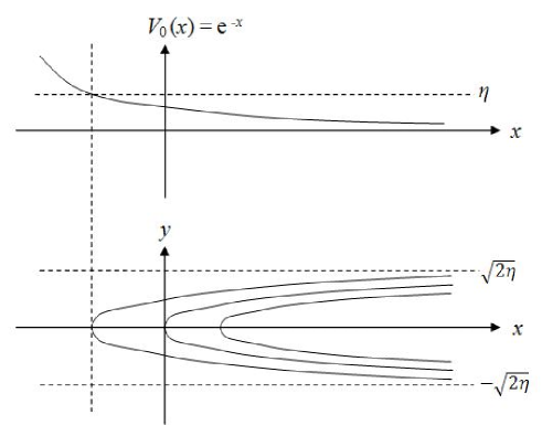
H ( I , φ , y , x ) = ω I + y 2 2 + V 0 ( x ) + ε g ( φ ) V 1 ( x ) . 𝐻 𝐼 𝜑 𝑦 𝑥 𝜔 𝐼 superscript 𝑦 2 2 subscript 𝑉 0 𝑥 𝜀 𝑔 𝜑 subscript 𝑉 1 𝑥 H(I,\varphi,y,x)=\omega I+\frac{y^{2}}{2}+V_{0}(x)+\varepsilon g(\varphi)V_{1}(x).
Here y 𝑦 y x 𝑥 x I 𝐼 I φ 𝜑 \varphi V 0 ( x ) = e − x subscript 𝑉 0 𝑥 superscript e 𝑥 V_{0}(x)=\mathrm{e}^{-x} V 1 subscript 𝑉 1 V_{1} x → + ∞ → 𝑥 x\to+\infty V 1 ≡ e − x subscript 𝑉 1 superscript e 𝑥 V_{1}\equiv\mathrm{e}^{-x}
H 0 ( I , y , x ) = ω I + y 2 2 + V 0 ( x ) = ω I + y 2 2 + e − x . subscript 𝐻 0 𝐼 𝑦 𝑥 𝜔 𝐼 superscript 𝑦 2 2 subscript 𝑉 0 𝑥 𝜔 𝐼 superscript 𝑦 2 2 superscript e 𝑥 H_{0}(I,y,x)=\omega I+\frac{y^{2}}{2}+V_{0}(x)=\omega I+\frac{y^{2}}{2}+\mathrm{e}^{-x}.
Let H 0 ( I , y , x ) = ω I + y 2 2 + e − x = h 0 = const subscript 𝐻 0 𝐼 𝑦 𝑥 𝜔 𝐼 superscript 𝑦 2 2 superscript e 𝑥 subscript ℎ 0 const H_{0}(I,y,x)=\omega I+\dfrac{y^{2}}{2}+\mathrm{e}^{-x}=h_{0}=\mathrm{const}
Figure 10:
Take ξ ~ ~ 𝜉 \tilde{\xi} H 0 ( I , y , x ) = ω I + y 2 2 + e − x = h 0 subscript 𝐻 0 𝐼 𝑦 𝑥 𝜔 𝐼 superscript 𝑦 2 2 superscript e 𝑥 subscript ℎ 0 H_{0}(I,y,x)=\omega I+\dfrac{y^{2}}{2}+\mathrm{e}^{-x}=h_{0}
d x d ξ ~ = ∂ H 0 ∂ y = y . d 𝑥 d ~ 𝜉 subscript 𝐻 0 𝑦 𝑦 \frac{\mathrm{d}x}{\mathrm{d}\tilde{\xi}}=\frac{\partial H_{0}}{\partial y}=y.
So
1 2 ( d x d ξ ~ ) 2 + e − x = h 0 − ω I = η ~ . 1 2 superscript d 𝑥 d ~ 𝜉 2 superscript e 𝑥 subscript ℎ 0 𝜔 𝐼 ~ 𝜂 \frac{1}{2}\left(\frac{\mathrm{d}x}{\mathrm{d}\tilde{\xi}}\right)^{2}+\mathrm{e}^{-x}=h_{0}-\omega I=\tilde{\eta}.
Thus we can express x 𝑥 x y 𝑦 y ( ξ ~ , η ~ ) ~ 𝜉 ~ 𝜂 (\tilde{\xi},\tilde{\eta})
x = x ( ξ ~ , η ~ ) , y = y ( ξ ~ , η ~ ) formulae-sequence 𝑥 𝑥 ~ 𝜉 ~ 𝜂 𝑦 𝑦 ~ 𝜉 ~ 𝜂 x=x(\tilde{\xi},\tilde{\eta}),\quad y=y(\tilde{\xi},\tilde{\eta})
with initial data x 0 = x ( 0 , η ~ ) superscript 𝑥 0 𝑥 0 ~ 𝜂 x^{0}=x(0,\tilde{\eta}) y 0 = 2 ( η ~ − e − x 0 ) superscript 𝑦 0 2 ~ 𝜂 superscript e superscript 𝑥 0 y^{0}=\sqrt{2(\tilde{\eta}-\mathrm{e}^{-x^{0}})}
After solving differential equations, we can obtain the solutions as (see [7 ] )
x ( ξ ~ , η ~ ) = log ( 1 η ~ ( cosh η ~ / 2 ( ξ ~ − ξ ~ 0 ) ) 2 ) , y ( ξ ~ , η ~ ) = 2 η ~ tanh η ~ / 2 ( ξ ~ − ξ ~ 0 ) . formulae-sequence 𝑥 ~ 𝜉 ~ 𝜂 1 ~ 𝜂 superscript ~ 𝜂 2 ~ 𝜉 superscript ~ 𝜉 0 2 𝑦 ~ 𝜉 ~ 𝜂 2 ~ 𝜂 ~ 𝜂 2 ~ 𝜉 superscript ~ 𝜉 0 x(\tilde{\xi},\tilde{\eta})=\log\left(\frac{1}{\tilde{\eta}}\Big{(}\cosh\sqrt{\tilde{\eta}/2}\,\big{(}\tilde{\xi}-\tilde{\xi}^{0}\big{)}\Big{)}^{2}\right),\quad y(\tilde{\xi},\tilde{\eta})=\sqrt{2\tilde{\eta}}\,\tanh\sqrt{\tilde{\eta}/2}\,\big{(}\tilde{\xi}-\tilde{\xi}^{0}\big{)}.
For simplicity we take the initial value of ξ ~ ~ 𝜉 \tilde{\xi} ξ ~ 0 = 0 superscript ~ 𝜉 0 0 \tilde{\xi}^{0}=0 x 0 = x ( 0 , η ~ ) = log 1 η ~ superscript 𝑥 0 𝑥 0 ~ 𝜂 1 ~ 𝜂 x^{0}=x(0,\tilde{\eta})=\log\dfrac{1}{\tilde{\eta}} y 0 = 0 superscript 𝑦 0 0 y^{0}=0
Now after the canonical transformation of variables from ( x , y ) 𝑥 𝑦 (x,y) ( ξ ~ , η ~ ) ~ 𝜉 ~ 𝜂 (\tilde{\xi},\tilde{\eta}) H 0 subscript 𝐻 0 H_{0} K 0 ( ξ ~ , η ~ ) = ω I + η ~ subscript 𝐾 0 ~ 𝜉 ~ 𝜂 𝜔 𝐼 ~ 𝜂 K_{0}(\tilde{\xi},\tilde{\eta})=\omega I+\tilde{\eta}
K ( ξ ~ , η ~ , I , φ ) = ω I + η ~ + ε f ( ξ ~ , η ~ ) g ( φ ) 𝐾 ~ 𝜉 ~ 𝜂 𝐼 𝜑 𝜔 𝐼 ~ 𝜂 𝜀 𝑓 ~ 𝜉 ~ 𝜂 𝑔 𝜑 K(\tilde{\xi},\tilde{\eta},I,\varphi)=\omega I+\tilde{\eta}+\varepsilon f(\tilde{\xi},\tilde{\eta})g(\varphi)
with
f ( ξ ~ , η ~ ) = V 1 ( x ( ξ ~ , η ~ ) ) = e − log ( 1 η ~ ( cosh η ~ / 2 ξ ~ ) 2 ) = η ~ ( cosh η ~ / 2 ξ ~ ) 2 . 𝑓 ~ 𝜉 ~ 𝜂 subscript 𝑉 1 𝑥 ~ 𝜉 ~ 𝜂 superscript e 1 ~ 𝜂 superscript ~ 𝜂 2 ~ 𝜉 2 ~ 𝜂 superscript ~ 𝜂 2 ~ 𝜉 2 f(\tilde{\xi},\tilde{\eta})=V_{1}(x(\tilde{\xi},\tilde{\eta}))=\mathrm{e}^{-\log\left(\frac{1}{\tilde{\eta}}\left(\cosh\sqrt{\tilde{\eta}/2}\,\tilde{\xi}\right)^{2}\right)}=\frac{\tilde{\eta}}{\left(\cosh\sqrt{\tilde{\eta}/2}\,\tilde{\xi}\right)^{2}}.
The differential equations for describing the motion are
ξ ~ ˙ = ε + ε 2 ∂ f ( ξ ~ , η ~ ) ∂ η ~ g ( φ ) , ˙ ~ 𝜉 𝜀 superscript 𝜀 2 𝑓 ~ 𝜉 ~ 𝜂 ~ 𝜂 𝑔 𝜑 \displaystyle\dot{\tilde{\xi}}=\varepsilon+\varepsilon^{2}\frac{\partial f(\tilde{\xi},\tilde{\eta})}{\partial\tilde{\eta}}g(\varphi),
η ~ ˙ = − ε 2 ∂ f ( ξ ~ , η ~ ) ∂ ξ ~ g ( φ ) , ˙ ~ 𝜂 superscript 𝜀 2 𝑓 ~ 𝜉 ~ 𝜂 ~ 𝜉 𝑔 𝜑 \displaystyle\dot{\tilde{\eta}}=-\varepsilon^{2}\frac{\partial f(\tilde{\xi},\tilde{\eta})}{\partial\tilde{\xi}}g(\varphi),
I ˙ = − ε f ( ξ ~ , η ~ ) d g ( φ ) d φ , ˙ 𝐼 𝜀 𝑓 ~ 𝜉 ~ 𝜂 d 𝑔 𝜑 d 𝜑 \displaystyle\dot{I}=-\varepsilon f(\tilde{\xi},\tilde{\eta})\frac{\mathrm{d}g(\varphi)}{\mathrm{d}\varphi},
φ ˙ = ω . ˙ 𝜑 𝜔 \displaystyle\dot{\varphi}=\omega.
For g ( φ ) 𝑔 𝜑 g(\varphi) g ( φ ) 𝑔 𝜑 g(\varphi) | Im φ | < ρ Im 𝜑 𝜌 |\text{Im}\,\varphi|<\rho ρ > 0 𝜌 0 \rho>0
| g ( φ ) | ≤ 1 , for | Im φ | < ρ . formulae-sequence 𝑔 𝜑 1 for Im 𝜑 𝜌 |g(\varphi)|\leq 1,\quad\text{for}\ |\text{Im}\,\varphi|<\rho.
For f ( ξ ~ , η ~ ) 𝑓 ~ 𝜉 ~ 𝜂 f(\tilde{\xi},\tilde{\eta})
| f ( ξ ~ , η ~ ) | < const 1 + | ξ ~ | 2 + ν , 𝑓 ~ 𝜉 ~ 𝜂 const 1 superscript ~ 𝜉 2 𝜈 |f(\tilde{\xi},\tilde{\eta})|<\frac{\mathrm{const}}{1+|\tilde{\xi}|^{2+\nu}},
and
| ∂ f ( ξ ~ , η ~ ) ∂ ξ ~ | < const 1 + | ξ ~ | 2 + ν , 𝑓 ~ 𝜉 ~ 𝜂 ~ 𝜉 const 1 superscript ~ 𝜉 2 𝜈 \left|\frac{\partial f(\tilde{\xi},\tilde{\eta})}{\partial\tilde{\xi}}\right|<\frac{\mathrm{const}}{1+|\tilde{\xi}|^{2+\nu}},
| ∂ f ( ξ ~ , η ~ ) ∂ η ~ | < const 1 + | ξ ~ | 2 + ν . 𝑓 ~ 𝜉 ~ 𝜂 ~ 𝜂 const 1 superscript ~ 𝜉 2 𝜈 \left|\frac{\partial f(\tilde{\xi},\tilde{\eta})}{\partial\tilde{\eta}}\right|<\frac{\mathrm{const}}{1+|\tilde{\xi}|^{2+\nu}}.
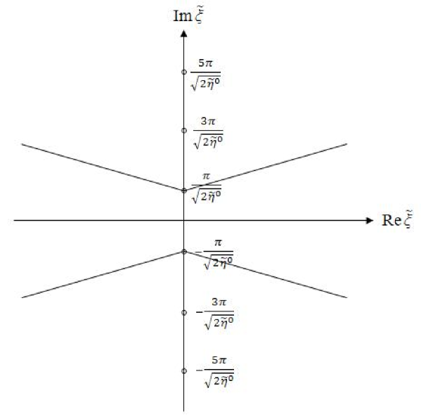
Take D I subscript 𝐷 𝐼 D_{I} I ∗ subscript 𝐼 I_{*} D φ subscript 𝐷 𝜑 D_{\varphi} | Im φ | < ρ Im 𝜑 𝜌 |\text{Im}\,\varphi|<\rho ξ ~ ~ 𝜉 \tilde{\xi} f ( ξ ~ , η ~ ) 𝑓 ~ 𝜉 ~ 𝜂 f(\tilde{\xi},\tilde{\eta})
f ( ξ ~ , η ~ ) = η ~ ( cosh η ~ / 2 ξ ~ ) 2 = 4 η ~ ( e η ~ / 2 ξ ~ + e − η ~ / 2 ξ ~ ) 2 . 𝑓 ~ 𝜉 ~ 𝜂 ~ 𝜂 superscript ~ 𝜂 2 ~ 𝜉 2 4 ~ 𝜂 superscript superscript e ~ 𝜂 2 ~ 𝜉 superscript e ~ 𝜂 2 ~ 𝜉 2 f(\tilde{\xi},\tilde{\eta})=\frac{\tilde{\eta}}{\left(\cosh\sqrt{\tilde{\eta}/2}\,\tilde{\xi}\right)^{2}}=\frac{4\tilde{\eta}}{\left(\mathrm{e}^{\sqrt{\tilde{\eta}/2}\,\tilde{\xi}}+\mathrm{e}^{-\sqrt{\tilde{\eta}/2}\,\tilde{\xi}}\right)^{2}}.
Points of singularities should satisfy
e η ~ / 2 ξ ~ + e − η ~ / 2 ξ ~ = 0 superscript e ~ 𝜂 2 ~ 𝜉 superscript e ~ 𝜂 2 ~ 𝜉 0 \displaystyle\mathrm{e}^{\sqrt{\tilde{\eta}/2}\,\tilde{\xi}}+\mathrm{e}^{-\sqrt{\tilde{\eta}/2}\,\tilde{\xi}}=0
e 2 η ~ / 2 ξ ~ + 1 = 0 superscript e 2 ~ 𝜂 2 ~ 𝜉 1 0 \displaystyle\mathrm{e}^{2\sqrt{\tilde{\eta}/2}\,\tilde{\xi}}+1=0
e 2 η ~ ξ ~ = − 1 superscript e 2 ~ 𝜂 ~ 𝜉 1 \displaystyle\mathrm{e}^{\sqrt{2\tilde{\eta}}\,\tilde{\xi}}=-1
e Re 2 η ~ ξ ~ ( cos Im 2 η ~ ξ ~ + i sin Im 2 η ~ ξ ~ ) = − 1 superscript e Re 2 ~ 𝜂 ~ 𝜉 Im 2 ~ 𝜂 ~ 𝜉 i Im 2 ~ 𝜂 ~ 𝜉 1 \displaystyle\mathrm{e}^{\text{Re}\,\sqrt{2\tilde{\eta}}\,\tilde{\xi}}\,\left(\cos\text{Im}\,\sqrt{2\tilde{\eta}}\,\tilde{\xi}+\mathrm{i}\sin\text{Im}\,\sqrt{2\tilde{\eta}}\,\tilde{\xi}\right)=-1
So cos Im 2 η ~ ξ ~ = − e − Re 2 η ~ ξ ~ < 0 , Im 2 ~ 𝜂 ~ 𝜉 superscript e Re 2 ~ 𝜂 ~ 𝜉 0 \displaystyle\cos\text{Im}\,\sqrt{2\tilde{\eta}}\,\tilde{\xi}=-\mathrm{e}^{-\text{Re}\,\sqrt{2\tilde{\eta}}\,\tilde{\xi}}<0,
sin Im 2 η ~ ξ ~ = 0 . Im 2 ~ 𝜂 ~ 𝜉 0 \displaystyle\sin\text{Im}\,\sqrt{2\tilde{\eta}}\,\tilde{\xi}=0.
Therefore, Im 2 η ~ ξ ~ = ( 2 k + 1 ) π , k ∈ ℤ , formulae-sequence Im 2 ~ 𝜂 ~ 𝜉 2 𝑘 1 𝜋 𝑘 ℤ \displaystyle\text{Im}\,\sqrt{2\tilde{\eta}}\,\tilde{\xi}=(2k+1)\pi,\quad k\in\mathbb{Z},
and Re 2 η ~ ξ ~ = 0 . Re 2 ~ 𝜂 ~ 𝜉 0 \displaystyle\text{Re}\,\sqrt{2\tilde{\eta}}\,\tilde{\xi}=0.
Thus
2 η ~ ξ ~ = ( 2 k + 1 ) π i , k ∈ ℤ . formulae-sequence 2 ~ 𝜂 ~ 𝜉 2 𝑘 1 𝜋 i 𝑘 ℤ \sqrt{2\tilde{\eta}}\,\tilde{\xi}=(2k+1)\pi\mathrm{i},\quad k\in\mathbb{Z}.
The domain of η ~ ~ 𝜂 \tilde{\eta} D η ~ subscript 𝐷 ~ 𝜂 D_{\tilde{\eta}} η ~ ∗ subscript ~ 𝜂 \tilde{\eta}_{*} η ~ 0 ∈ D η ~ superscript ~ 𝜂 0 subscript 𝐷 ~ 𝜂 \tilde{\eta}^{0}\in D_{\tilde{\eta}}
ξ ~ = ( 2 k + 1 ) π 2 η ~ 0 i , k ∈ ℤ . formulae-sequence ~ 𝜉 2 𝑘 1 𝜋 2 superscript ~ 𝜂 0 i 𝑘 ℤ \tilde{\xi}=(2k+1)\frac{\pi}{\sqrt{2\tilde{\eta}^{0}}\;}\,\mathrm{i},\quad k\in\mathbb{Z}.
From the above conclusion, if we take ξ ~ ~ 𝜉 \tilde{\xi}
D ξ ~ = { ξ ~ : | Im ξ ~ | < π 2 η ~ 0 + δ | Re ξ ~ | } , subscript 𝐷 ~ 𝜉 conditional-set ~ 𝜉 Im ~ 𝜉 𝜋 2 superscript ~ 𝜂 0 𝛿 Re ~ 𝜉 D_{\tilde{\xi}}=\{\tilde{\xi}\colon|\text{Im}\,\tilde{\xi}|<\frac{\pi}{\sqrt{2\tilde{\eta}^{0}}\;}+\delta|\text{Re}\,\tilde{\xi}|\},
where δ 𝛿 \delta f ( ξ ~ , η ~ ) 𝑓 ~ 𝜉 ~ 𝜂 f(\tilde{\xi},\tilde{\eta}) η ~ ∈ D η ~ ~ 𝜂 subscript 𝐷 ~ 𝜂 \tilde{\eta}\in D_{\tilde{\eta}}
The following figure shows the boundary of domain D ξ ~ subscript 𝐷 ~ 𝜉 D_{\tilde{\xi}}
Figure 11:
We can find the level lines
Im ∫ 0 ξ ~ ω d ξ ~ 1 = ω Im ξ ~ = B = const , 0 ≤ | B | ≤ γ formulae-sequence Im superscript subscript 0 ~ 𝜉 𝜔 differential-d subscript ~ 𝜉 1 𝜔 Im ~ 𝜉 𝐵 const 0 𝐵 𝛾 \text{Im}\,\int\limits_{0}^{\tilde{\xi}}\omega\,\mathrm{d}\tilde{\xi}_{1}=\omega\text{Im}\,\tilde{\xi}=B=\mathrm{const},\quad 0\leq|B|\leq\gamma
lying in the domain D ξ ~ subscript 𝐷 ~ 𝜉 D_{\tilde{\xi}} γ 𝛾 \gamma
γ < π ω 2 η ~ 0 , for such definition of η ~ 0 . 𝛾 𝜋 𝜔 2 superscript ~ 𝜂 0 for such definition of subscript ~ 𝜂 0
\gamma<\frac{\pi\omega}{\sqrt{2\tilde{\eta}^{0}}},\quad\rm{for\ such\ definition\ of\ \tilde{\eta}_{0}}.
According to Theorem 1, the accuracy of conservation of adiabatic invariant Δ I Δ 𝐼 \Delta I
Δ I = O ( e − γ ε ) . Δ 𝐼 𝑂 superscript e 𝛾 𝜀 \Delta I=O(\mathrm{e}^{-\frac{\gamma}{\varepsilon}}).
This estimate coincides with that in [7 ] , where it was obtained by a different method.
5 Proof of the Theorem
The original system is described by Hamiltonian
H ( I , φ , y , x ) = H 0 ( I , y , x ) + ε H 1 ( I , φ , y , x ) 𝐻 𝐼 𝜑 𝑦 𝑥 subscript 𝐻 0 𝐼 𝑦 𝑥 𝜀 subscript 𝐻 1 𝐼 𝜑 𝑦 𝑥 H(I,\varphi,y,x)=H_{0}(I,y,x)+\varepsilon H_{1}(I,\varphi,y,x)
with motion in time t 𝑡 t
I ˙ = − ε ∂ H 1 ∂ φ , φ ˙ = ∂ H 0 ∂ I + ε ∂ H 1 ∂ I , formulae-sequence ˙ 𝐼 𝜀 subscript 𝐻 1 𝜑 ˙ 𝜑 subscript 𝐻 0 𝐼 𝜀 subscript 𝐻 1 𝐼 \displaystyle\dot{I}=-\varepsilon\frac{\partial H_{1}}{\partial\varphi},\quad\dot{\varphi}=\frac{\partial H_{0}}{\partial I}+\varepsilon\frac{\partial H_{1}}{\partial I},
y ˙ = − ε ( ∂ H 0 ∂ x + ε ∂ H 1 ∂ x ) , x ˙ = ε ( ∂ H 0 ∂ y + ε ∂ H 1 ∂ y ) . formulae-sequence ˙ 𝑦 𝜀 subscript 𝐻 0 𝑥 𝜀 subscript 𝐻 1 𝑥 ˙ 𝑥 𝜀 subscript 𝐻 0 𝑦 𝜀 subscript 𝐻 1 𝑦 \displaystyle\dot{y}=-\varepsilon\left(\frac{\partial H_{0}}{\partial x}+\varepsilon\frac{\partial H_{1}}{\partial x}\right),\quad\dot{x}=\varepsilon\left(\frac{\partial H_{0}}{\partial y}+\varepsilon\frac{\partial H_{1}}{\partial y}\right).
As the frequency ω 0 ( I , y , x ) = ∂ H 0 ( I , y , x ) ∂ I subscript 𝜔 0 𝐼 𝑦 𝑥 subscript 𝐻 0 𝐼 𝑦 𝑥 𝐼 \omega_{0}(I,y,x)=\displaystyle\frac{\partial H_{0}(I,y,x)}{\partial I} D 𝐷 D I 𝐼 I H 𝐻 H φ 𝜑 \varphi y 𝑦 y x 𝑥 x H ( I , φ , y , x ) = h 0 , h 0 = const formulae-sequence 𝐻 𝐼 𝜑 𝑦 𝑥 subscript ℎ 0 subscript ℎ 0 const H(I,\varphi,y,x)=h_{0},\ h_{0}=\mathrm{const}
− I ( y , x , φ , h 0 ) = F 0 ( y , x , h 0 ) + ε F 1 ( y , x , φ , h 0 ) . 𝐼 𝑦 𝑥 𝜑 subscript ℎ 0 subscript 𝐹 0 𝑦 𝑥 subscript ℎ 0 𝜀 subscript 𝐹 1 𝑦 𝑥 𝜑 subscript ℎ 0 -I(y,x,\varphi,h_{0})=F_{0}(y,x,h_{0})+\varepsilon F_{1}(y,x,\varphi,h_{0}).
Here ( − I ) 𝐼 (-I) φ 𝜑 \varphi ( y , x ) 𝑦 𝑥 (y,x) D ~ x y subscript ~ 𝐷 𝑥 𝑦 \widetilde{D}_{xy} D ~ x y + δ x y subscript ~ 𝐷 𝑥 𝑦 subscript 𝛿 𝑥 𝑦 \widetilde{D}_{xy}+\delta_{xy}
D ~ x y = { ( y , x ) : { y = Y ( τ , I 0 , h 0 ) x = X ( τ , I 0 , h 0 ) , τ ∈ D τ , I 0 ∈ D I } , subscript ~ 𝐷 𝑥 𝑦 conditional-set 𝑦 𝑥 formulae-sequence cases 𝑦 𝑌 𝜏 subscript 𝐼 0 subscript ℎ 0 𝑥 𝑋 𝜏 subscript 𝐼 0 subscript ℎ 0 𝜏
subscript 𝐷 𝜏 subscript 𝐼 0 subscript 𝐷 𝐼 \widetilde{D}_{xy}=\bigg{\{}(y,x)\colon\Big{\{}\begin{array}[]{c}y=Y(\tau,I_{0},h_{0})\\
x=X(\tau,I_{0},h_{0})\end{array}\!,\ \tau\in D_{\tau},\ I_{0}\in D_{I}\bigg{\}},
and δ x y subscript 𝛿 𝑥 𝑦 \delta_{xy}
We do not indicate dependence of Y 𝑌 Y X 𝑋 X ε 𝜀 \varepsilon
d y d φ = − ε ( ∂ F 0 ∂ x + ε ∂ F 1 ∂ x ) , d x d φ = ε ( ∂ F 0 ∂ y + ε ∂ F 1 ∂ y ) . formulae-sequence d 𝑦 d 𝜑 𝜀 subscript 𝐹 0 𝑥 𝜀 subscript 𝐹 1 𝑥 d 𝑥 d 𝜑 𝜀 subscript 𝐹 0 𝑦 𝜀 subscript 𝐹 1 𝑦 \frac{\mathrm{d}y}{\mathrm{d}\varphi}=-\varepsilon\left(\frac{\partial F_{0}}{\partial x}+\varepsilon\frac{\partial F_{1}}{\partial x}\right),\quad\frac{\mathrm{d}x}{\mathrm{d}\varphi}=\varepsilon\left(\frac{\partial F_{0}}{\partial y}+\varepsilon\frac{\partial F_{1}}{\partial y}\right).
Since we know functions H 0 subscript 𝐻 0 H_{0} H 1 subscript 𝐻 1 H_{1} D 𝐷 D F 0 subscript 𝐹 0 F_{0} F 1 subscript 𝐹 1 F_{1} D φ × ( D ~ x y + δ x y ) subscript 𝐷 𝜑 subscript ~ 𝐷 𝑥 𝑦 subscript 𝛿 𝑥 𝑦 D_{\varphi}\times(\widetilde{D}_{xy}+\delta_{xy})
Now consider the approximate system with Hamiltonian
F 0 ( y , x , h 0 ) = − I 0 . subscript 𝐹 0 𝑦 𝑥 subscript ℎ 0 subscript 𝐼 0 F_{0}(y,x,h_{0})=-I_{0}.
Introduce slow time ξ = ε φ 𝜉 𝜀 𝜑 \xi=\varepsilon\varphi
d y d ξ = − ∂ F 0 ∂ x , d x d ξ = ∂ F 0 ∂ y . formulae-sequence d 𝑦 d 𝜉 subscript 𝐹 0 𝑥 d 𝑥 d 𝜉 subscript 𝐹 0 𝑦 \frac{\mathrm{d}y}{\mathrm{d}\xi}=-\frac{\partial F_{0}}{\partial x},\quad\frac{\mathrm{d}x}{\mathrm{d}\xi}=\frac{\partial F_{0}}{\partial y}.
We can find the solution for the above approximate system:
{ y = Y ^ ( ξ , I 0 , h 0 ) x = X ^ ( ξ , I 0 , h 0 ) I 0 ∈ D I , h 0 ∈ D h . formulae-sequence cases 𝑦 ^ 𝑌 𝜉 subscript 𝐼 0 subscript ℎ 0 missing-subexpression missing-subexpression 𝑥 ^ 𝑋 𝜉 subscript 𝐼 0 subscript ℎ 0 missing-subexpression missing-subexpression subscript 𝐼 0
subscript 𝐷 𝐼 subscript ℎ 0 subscript 𝐷 ℎ \left\{\begin{array}[]{ccc}y=\widehat{Y}(\xi,I_{0},h_{0})\\
x=\widehat{X}(\xi,I_{0},h_{0})\end{array}\right.\qquad I_{0}\in D_{I},\quad h_{0}\in D_{h}.
In what follows, we do not indicate the dependence on constant h 0 subscript ℎ 0 h_{0} Y ( τ , I 0 ) 𝑌 𝜏 subscript 𝐼 0 Y(\tau,I_{0}) X ( τ , I 0 ) 𝑋 𝜏 subscript 𝐼 0 X(\tau,I_{0}) Y ^ ( ξ , I 0 ) ^ 𝑌 𝜉 subscript 𝐼 0 \widehat{Y}(\xi,I_{0}) X ^ ( ξ , I 0 ) ^ 𝑋 𝜉 subscript 𝐼 0 \widehat{X}(\xi,I_{0})
ξ = ∫ 0 τ ω 0 ( I 0 , Y ( τ 1 , I 0 ) , X ( τ 1 , I 0 ) ) d τ 1 . 𝜉 superscript subscript 0 𝜏 subscript 𝜔 0 subscript 𝐼 0 𝑌 subscript 𝜏 1 subscript 𝐼 0 𝑋 subscript 𝜏 1 subscript 𝐼 0 differential-d subscript 𝜏 1 \xi=\int\limits_{0}^{\tau}\omega_{0}(I_{0},Y(\tau_{1},I_{0}),X(\tau_{1},I_{0}))\,\mathrm{d}\tau_{1}.
Solution Y ^ ( ξ , I 0 ) ^ 𝑌 𝜉 subscript 𝐼 0 \widehat{Y}(\xi,I_{0}) X ^ ( ξ , I 0 ) ^ 𝑋 𝜉 subscript 𝐼 0 \widehat{X}(\xi,I_{0}) D ξ subscript 𝐷 𝜉 D_{\xi} ξ 𝜉 \xi D ξ subscript 𝐷 𝜉 D_{\xi}
Im ω 0 ( I 0 , Y ( τ , I 0 ) , X ( τ , I 0 ) ) ⇉ 0 , as Re τ → ± ∞ , Im I 0 → 0 . formulae-sequence ⇉ Im subscript 𝜔 0 subscript 𝐼 0 𝑌 𝜏 subscript 𝐼 0 𝑋 𝜏 subscript 𝐼 0 0 formulae-sequence → as Re 𝜏 plus-or-minus → Im subscript 𝐼 0 0 \mathrm{Im}\ \omega_{0}(I_{0},Y(\tau,I_{0}),X(\tau,I_{0}))\rightrightarrows 0,\quad\mathrm{as}\ \mathrm{Re}\;\tau\to\pm\infty,\ \mathrm{Im}\;I_{0}\to 0.
It implies that ω 0 subscript 𝜔 0 \omega_{0} I 0 subscript 𝐼 0 \,I_{0} I 0 subscript 𝐼 0 I_{0} ω ± ( Re I 0 ) subscript 𝜔 plus-or-minus Re subscript 𝐼 0 \omega_{\pm}(\mathrm{Re}\,I_{0})
ω 0 ( I 0 , Y ( τ 1 , I 0 ) , X ( τ 1 , I 0 ) ) ⇉ ω ± ( Re I 0 ) , as Re τ → ± ∞ , Im I 0 → 0 . formulae-sequence ⇉ subscript 𝜔 0 subscript 𝐼 0 𝑌 subscript 𝜏 1 subscript 𝐼 0 𝑋 subscript 𝜏 1 subscript 𝐼 0 subscript 𝜔 plus-or-minus Re subscript 𝐼 0 formulae-sequence → as Re 𝜏 plus-or-minus → Im subscript 𝐼 0 0 \omega_{0}(I_{0},Y(\tau_{1},I_{0}),X(\tau_{1},I_{0}))\rightrightarrows\omega_{\pm}(\mathrm{Re}\,I_{0}),\quad\mathrm{as}\ \mathrm{Re}\,\tau\to\pm\infty,\ \mathrm{Im}\,I_{0}\to 0.
Lemma 5.1 .
For I 0 ∈ D I subscript 𝐼 0 subscript 𝐷 𝐼 I_{0}\in D_{I} D τ subscript 𝐷 𝜏 D_{\tau} τ ↦ ξ maps-to 𝜏 𝜉 \tau\mapsto\xi
ξ = ∫ 0 τ ω 0 ( I 0 , Y ( τ 1 , I 0 ) , X ( τ 1 , I 0 ) ) d τ 1 𝜉 superscript subscript 0 𝜏 subscript 𝜔 0 subscript 𝐼 0 𝑌 subscript 𝜏 1 subscript 𝐼 0 𝑋 subscript 𝜏 1 subscript 𝐼 0 differential-d subscript 𝜏 1 \xi=\int\limits_{0}^{\tau}\omega_{0}(I_{0},Y(\tau_{1},I_{0}),X(\tau_{1},I_{0}))\,\mathrm{d}\tau_{1}
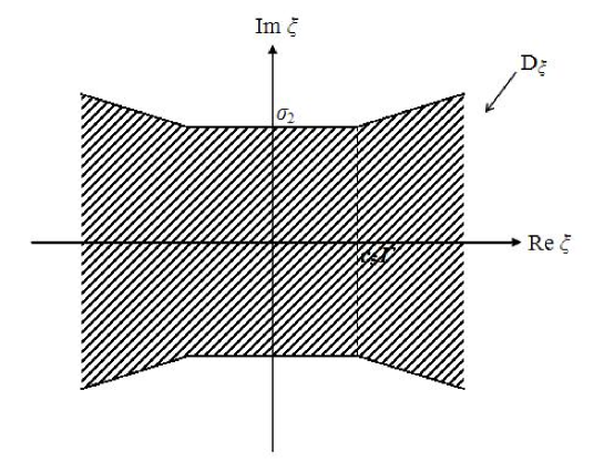
is a strip around the real axis that contains a domain
D ξ = { ξ : { | Im ξ | < σ 1 + δ 1 | Re ξ | , | Re ξ | > c 5 Γ | Im ξ | < σ 2 , | Re ξ | ≤ c 5 Γ } D_{\xi}=\bigg{\{}\xi\colon\Big{\{}\begin{array}[]{lc}|\mathrm{Im}\;\xi|<\sigma_{1}+\delta_{1}|\mathrm{Re}\;\xi|,&|\mathrm{Re}\;\xi|>c_{5}\Gamma\\
|\mathrm{Im}\;\xi|<\sigma_{2},&|\mathrm{Re}\;\xi|\leq c_{5}\Gamma\end{array}\bigg{\}}
Figure 12 :
where σ 1 subscript 𝜎 1 \sigma_{1} , σ 2 subscript 𝜎 2 \sigma_{2} , δ 1 subscript 𝛿 1 \delta_{1} , c 5 subscript 𝑐 5 c_{5} are positive constants and σ 2 = σ 1 + δ 1 ⋅ c 5 Γ subscript 𝜎 2 subscript 𝜎 1 ⋅ subscript 𝛿 1 subscript 𝑐 5 Γ \sigma_{2}=\sigma_{1}+\delta_{1}\cdot c_{5}\Gamma for continuity. Straight lines Im ξ = ± γ Im 𝜉 plus-or-minus 𝛾 \mathrm{Im}\,\xi=\pm\gamma lie in D ξ subscript 𝐷 𝜉 D_{\xi} and have a positive distance from the boundary of D ξ subscript 𝐷 𝜉 D_{\xi} (i.e. γ < σ 2 𝛾 subscript 𝜎 2 \gamma<\sigma_{2} ).
Lemma 5.2 .
The function F 1 ( y , x , φ ) subscript 𝐹 1 𝑦 𝑥 𝜑 F_{1}(y,x,\varphi)
| F 1 ( Y ^ ( ξ , I 0 ) , X ^ ( ξ , I 0 ) , φ ) | < const 1 + | ξ | 2 + ν . subscript 𝐹 1 ^ 𝑌 𝜉 subscript 𝐼 0 ^ 𝑋 𝜉 subscript 𝐼 0 𝜑 const 1 superscript 𝜉 2 𝜈 |F_{1}(\widehat{Y}(\xi,I_{0}),\widehat{X}(\xi,I_{0}),\varphi)|<\frac{\mathrm{const}}{1+|\xi|^{2+\nu}}.
Proof.
First of all let us list two forms of Hamiltonian:
H 0 ( I , y , x ) + ε H 1 ( I , φ , y , x ) = h 0 , subscript 𝐻 0 𝐼 𝑦 𝑥 𝜀 subscript 𝐻 1 𝐼 𝜑 𝑦 𝑥 subscript ℎ 0 \displaystyle H_{0}(I,y,x)+\varepsilon H_{1}(I,\varphi,y,x)=h_{0},
− I = F 0 ( y , x ) + ε F 1 ( y , x , φ ) . 𝐼 subscript 𝐹 0 𝑦 𝑥 𝜀 subscript 𝐹 1 𝑦 𝑥 𝜑 \displaystyle-I=F_{0}(y,x)+\varepsilon F_{1}(y,x,\varphi).
Therefore, we have
H 0 ( − ( F 0 + ε F 1 ) , y , x ) + ε H 1 ( − ( F 0 + ε F 1 ) , φ , y , x ) = h 0 . subscript 𝐻 0 subscript 𝐹 0 𝜀 subscript 𝐹 1 𝑦 𝑥 𝜀 subscript 𝐻 1 subscript 𝐹 0 𝜀 subscript 𝐹 1 𝜑 𝑦 𝑥 subscript ℎ 0 \displaystyle H_{0}(-(F_{0}+\varepsilon F_{1}),y,x)+\varepsilon H_{1}(-(F_{0}+\varepsilon F_{1}),\varphi,y,x)=h_{0}.
Then let ε = 0 : : Then let 𝜀 0 absent \displaystyle\textup{Then let}\ \varepsilon=0: H 0 ( − F 0 , y , x ) = h 0 . subscript 𝐻 0 subscript 𝐹 0 𝑦 𝑥 subscript ℎ 0 \displaystyle H_{0}(-F_{0},y,x)=h_{0}.
So
H 0 ( − ( F 0 + ε F 1 ) , y , x ) + ε H 1 ( − ( F 0 + ε F 1 ) , φ , y , x ) = H 0 ( − F 0 , y , x ) , subscript 𝐻 0 subscript 𝐹 0 𝜀 subscript 𝐹 1 𝑦 𝑥 𝜀 subscript 𝐻 1 subscript 𝐹 0 𝜀 subscript 𝐹 1 𝜑 𝑦 𝑥 subscript 𝐻 0 subscript 𝐹 0 𝑦 𝑥 \displaystyle H_{0}(-(F_{0}+\varepsilon F_{1}),y,x)+\varepsilon H_{1}(-(F_{0}+\varepsilon F_{1}),\varphi,y,x)=H_{0}(-F_{0},y,x),
H 0 ( − ( F 0 + ε F 1 ) , y , x ) − H 0 ( − F 0 , y , x ) = − ε H 1 ( − ( F 0 + ε F 1 ) , φ , y , x ) . subscript 𝐻 0 subscript 𝐹 0 𝜀 subscript 𝐹 1 𝑦 𝑥 subscript 𝐻 0 subscript 𝐹 0 𝑦 𝑥 𝜀 subscript 𝐻 1 subscript 𝐹 0 𝜀 subscript 𝐹 1 𝜑 𝑦 𝑥 \displaystyle H_{0}(-(F_{0}+\varepsilon F_{1}),y,x)-H_{0}(-F_{0},y,x)=-\varepsilon H_{1}(-(F_{0}+\varepsilon F_{1}),\varphi,y,x).
Applying the intermediate value theorem here, we get that there exist some value I ~ ~ 𝐼 \widetilde{I}
∂ H 0 ( I ~ , y , x ) ∂ I ⋅ ( − ε F 1 ) = − ε H 1 ( − ( F 0 + ε F 1 ) , φ , y , x ) ⋅ subscript 𝐻 0 ~ 𝐼 𝑦 𝑥 𝐼 𝜀 subscript 𝐹 1 𝜀 subscript 𝐻 1 subscript 𝐹 0 𝜀 subscript 𝐹 1 𝜑 𝑦 𝑥 \displaystyle\frac{\partial H_{0}(\widetilde{I},y,x)}{\partial I}\cdot(-\varepsilon F_{1})=-\varepsilon H_{1}(-(F_{0}+\varepsilon F_{1}),\varphi,y,x)
so F 1 ( y , x , φ ) = 1 ∂ H 0 ( I ~ , y , x ) ∂ I ⋅ H 1 ( I , φ , y , x ) subscript 𝐹 1 𝑦 𝑥 𝜑 ⋅ 1 subscript 𝐻 0 ~ 𝐼 𝑦 𝑥 𝐼 subscript 𝐻 1 𝐼 𝜑 𝑦 𝑥 \displaystyle F_{1}(y,x,\varphi)=\frac{1}{\displaystyle\frac{\partial H_{0}(\widetilde{I},y,x)}{\partial I}}\cdot H_{1}(I,\varphi,y,x)
We know from assumptions that
| ω 0 | = | ∂ H 0 ∂ I | > const subscript 𝜔 0 subscript 𝐻 0 𝐼 const \displaystyle|\omega_{0}|=\left|\frac{\partial H_{0}}{\partial I}\right|>\mathrm{const}
and | H 1 ( I , φ , Y ( τ , I 0 ) , X ( τ , I 0 ) ) | < c 1 + | ∫ 0 τ ω 0 ( I 0 , Y ( τ 1 , I 0 ) , X ( τ 1 , I 0 ) ) d τ 1 | 2 + ν subscript 𝐻 1 𝐼 𝜑 𝑌 𝜏 subscript 𝐼 0 𝑋 𝜏 subscript 𝐼 0 𝑐 1 superscript superscript subscript 0 𝜏 subscript 𝜔 0 subscript 𝐼 0 𝑌 subscript 𝜏 1 subscript 𝐼 0 𝑋 subscript 𝜏 1 subscript 𝐼 0 differential-d subscript 𝜏 1 2 𝜈 \displaystyle|H_{1}(I,\varphi,Y(\tau,I_{0}),X(\tau,I_{0}))|<\frac{c}{1+\left|\int\limits_{0}^{\tau}\omega_{0}(I_{0},Y(\tau_{1},I_{0}),X(\tau_{1},I_{0}))\,\mathrm{d}\tau_{1}\right|^{2+\nu}}
Therefore,
| F 1 ( Y ^ ( ξ , I 0 ) , X ^ ( ξ , I 0 ) , φ ) | subscript 𝐹 1 ^ 𝑌 𝜉 subscript 𝐼 0 ^ 𝑋 𝜉 subscript 𝐼 0 𝜑 \displaystyle|F_{1}(\widehat{Y}(\xi,I_{0}),\widehat{X}(\xi,I_{0}),\varphi)| < \displaystyle< const ⋅ | H 1 ( I , φ , Y ( τ , I 0 ) , X ( τ , I 0 ) ) | ⋅ const subscript 𝐻 1 𝐼 𝜑 𝑌 𝜏 subscript 𝐼 0 𝑋 𝜏 subscript 𝐼 0 \displaystyle\mathrm{const}\cdot|H_{1}(I,\varphi,Y(\tau,I_{0}),X(\tau,I_{0}))|
< \displaystyle< const 1 + | ξ | 2 + ν . const 1 superscript 𝜉 2 𝜈 \displaystyle\frac{\mathrm{const}}{1+|\xi|^{2+\nu}}.
Corollary 5.1 .
For φ ∈ D ~ φ = D φ − δ φ 𝜑 subscript ~ 𝐷 𝜑 subscript 𝐷 𝜑 subscript 𝛿 𝜑 \varphi\in\widetilde{D}_{\varphi}=D_{\varphi}-\delta_{\varphi} ξ ∈ D ~ ξ = D ξ − δ ξ 𝜉 subscript ~ 𝐷 𝜉 subscript 𝐷 𝜉 subscript 𝛿 𝜉 \xi\in\widetilde{D}_{\xi}=D_{\xi}-\delta_{\xi}
| ∂ F 1 ( Y ^ ( ξ , I 0 ) , X ^ ( ξ , I 0 ) , φ , h 0 ) ∂ φ | < const 1 + | ξ | 2 + ν , subscript 𝐹 1 ^ 𝑌 𝜉 subscript 𝐼 0 ^ 𝑋 𝜉 subscript 𝐼 0 𝜑 subscript ℎ 0 𝜑 const 1 superscript 𝜉 2 𝜈 \left|\frac{\partial F_{1}(\widehat{Y}(\xi,I_{0}),\widehat{X}(\xi,I_{0}),\varphi,h_{0})}{\partial\varphi}\right|<\frac{\mathrm{const}}{1+|\xi|^{2+\nu}},
| ∂ F 1 ( Y ^ ( ξ , I 0 ) , X ^ ( ξ , I 0 ) , φ , h 0 ) ∂ ξ | < const 1 + | ξ | 2 + ν , subscript 𝐹 1 ^ 𝑌 𝜉 subscript 𝐼 0 ^ 𝑋 𝜉 subscript 𝐼 0 𝜑 subscript ℎ 0 𝜉 const 1 superscript 𝜉 2 𝜈 \left|\frac{\partial F_{1}(\widehat{Y}(\xi,I_{0}),\widehat{X}(\xi,I_{0}),\varphi,h_{0})}{\partial\xi}\right|<\frac{\mathrm{const}}{1+|\xi|^{2+\nu}},
where δ ξ subscript 𝛿 𝜉 \delta_{\xi}
Now let us draw the phase portrait of F 0 ( y , x ) = − I subscript 𝐹 0 𝑦 𝑥 𝐼 F_{0}(y,x)=-I
Figure 13:
and introduce new coordinates ( ξ , η ) 𝜉 𝜂 (\xi,\eta) η 𝜂 \eta F 0 subscript 𝐹 0 F_{0} F 0 = η subscript 𝐹 0 𝜂 F_{0}=\eta ξ 𝜉 \xi X ^ ( 0 , I ) ^ 𝑋 0 𝐼 \widehat{X}(0,I) Y ^ ( 0 , I ) ^ 𝑌 0 𝐼 \widehat{Y}(0,I) I 𝐼 I ( ξ , η ) ↦ ( x , y ) maps-to 𝜉 𝜂 𝑥 𝑦 (\xi,\eta)\mapsto(x,y)
Lemma 5.3 .
In the domain D ξ × D η subscript 𝐷 𝜉 subscript 𝐷 𝜂 D_{\xi}\times D_{\eta} D ξ subscript 𝐷 𝜉 D_{\xi} D η subscript 𝐷 𝜂 D_{\eta} − I ∗ subscript 𝐼 -I_{*} ( ξ , η ) ↦ ( x , y ) maps-to 𝜉 𝜂 𝑥 𝑦 (\xi,\eta)\mapsto(x,y)
Proof.
With map ( ξ , η ) ↦ ( x , y ) maps-to 𝜉 𝜂 𝑥 𝑦 (\xi,\eta)\mapsto(x,y) x 𝑥 x y 𝑦 y ξ 𝜉 \xi η 𝜂 \eta
x = x ( ξ , η ) , y = y ( ξ , η ) . formulae-sequence 𝑥 𝑥 𝜉 𝜂 𝑦 𝑦 𝜉 𝜂 x=x(\xi,\eta),\quad y=y(\xi,\eta).
From the motion above, we have obtained the relations:
∂ x ∂ ξ = ∂ F 0 ∂ y , ∂ y ∂ ξ = − ∂ F 0 ∂ x . formulae-sequence 𝑥 𝜉 subscript 𝐹 0 𝑦 𝑦 𝜉 subscript 𝐹 0 𝑥 \frac{\partial x}{\partial\xi}=\frac{\partial F_{0}}{\partial y},\quad\frac{\partial y}{\partial\xi}=-\frac{\partial F_{0}}{\partial x}.
Let us differentiate both sides of the Hamiltonian F 0 ( y , x , h 0 ) = η subscript 𝐹 0 𝑦 𝑥 subscript ℎ 0 𝜂 F_{0}(y,x,h_{0})=\eta η 𝜂 \eta
∂ F 0 ∂ y ∂ y ∂ η + ∂ F 0 ∂ x ∂ x ∂ η = 1 . subscript 𝐹 0 𝑦 𝑦 𝜂 subscript 𝐹 0 𝑥 𝑥 𝜂 1 \frac{\partial F_{0}}{\partial y}\frac{\partial y}{\partial\eta}+\frac{\partial F_{0}}{\partial x}\frac{\partial x}{\partial\eta}=1.
Replacing with corresponding derivatives, we get
∂ x ∂ ξ ∂ y ∂ η − ∂ y ∂ ξ ∂ x ∂ η = 1 . 𝑥 𝜉 𝑦 𝜂 𝑦 𝜉 𝑥 𝜂 1 \frac{\partial x}{\partial\xi}\frac{\partial y}{\partial\eta}-\frac{\partial y}{\partial\xi}\frac{\partial x}{\partial\eta}=1.
That is indeed the Jacobi determinant:
D ( x , y ) D ( ξ , η ) = det | ∂ x ∂ ξ ∂ x ∂ η ∂ y ∂ ξ ∂ y ∂ η | = 1 . 𝐷 𝑥 𝑦 𝐷 𝜉 𝜂 𝑥 𝜉 𝑥 𝜂 missing-subexpression missing-subexpression 𝑦 𝜉 𝑦 𝜂 1 \frac{D(x,y)}{D(\xi,\eta)}=\det\left|\begin{array}[]{cc}\dfrac{\partial x}{\partial\xi}&\dfrac{\partial x}{\partial\eta}\\
\\
\dfrac{\partial y}{\partial\xi}&\dfrac{\partial y}{\partial\eta}\end{array}\right|=1.
Therefore, ( x , y ) ↦ ( ξ , η ) maps-to 𝑥 𝑦 𝜉 𝜂 (x,y)\mapsto(\xi,\eta)
After this transformation, the new Hamiltonian has the form
− I ( η , ξ , φ ) = η + ε G 1 ( η , ξ , φ ) . 𝐼 𝜂 𝜉 𝜑 𝜂 𝜀 subscript 𝐺 1 𝜂 𝜉 𝜑 -I(\eta,\xi,\varphi)=\eta+\varepsilon G_{1}(\eta,\xi,\varphi).
Function G 1 subscript 𝐺 1 G_{1}
| G 1 ( η , ξ , φ ) | < const 1 + | ξ | 2 + ν . subscript 𝐺 1 𝜂 𝜉 𝜑 const 1 superscript 𝜉 2 𝜈 |G_{1}(\eta,\xi,\varphi)|<\frac{\mathrm{const}}{1+|\xi|^{2+\nu}}.
Also from Cauchy estimate [5 ] , for η ∈ D ~ η = D η − δ η 𝜂 subscript ~ 𝐷 𝜂 subscript 𝐷 𝜂 subscript 𝛿 𝜂 \eta\in\widetilde{D}_{\eta}=D_{\eta}-\delta_{\eta} ξ ∈ D ~ ξ = D ξ − δ ξ 𝜉 subscript ~ 𝐷 𝜉 subscript 𝐷 𝜉 subscript 𝛿 𝜉 \xi\in\widetilde{D}_{\xi}=D_{\xi}-\delta_{\xi} φ ∈ D ~ φ 𝜑 subscript ~ 𝐷 𝜑 \varphi\in\widetilde{D}_{\varphi} δ η subscript 𝛿 𝜂 \delta_{\eta} δ ξ subscript 𝛿 𝜉 \delta_{\xi}
| ∂ G 1 ( η , ξ , φ ) ∂ φ | < const 1 + | ξ | 2 + ν , subscript 𝐺 1 𝜂 𝜉 𝜑 𝜑 const 1 superscript 𝜉 2 𝜈 \left|\frac{\partial G_{1}(\eta,\xi,\varphi)}{\partial\varphi}\right|<\frac{\mathrm{const}}{1+|\xi|^{2+\nu}},
| ∂ G 1 ( η , ξ , φ ) ∂ η | < const 1 + | ξ | 2 + ν , subscript 𝐺 1 𝜂 𝜉 𝜑 𝜂 const 1 superscript 𝜉 2 𝜈 \left|\frac{\partial G_{1}(\eta,\xi,\varphi)}{\partial\eta}\right|<\frac{\mathrm{const}}{1+|\xi|^{2+\nu}},
| ∂ G 1 ( η , ξ , φ ) ∂ ξ | < const 1 + | ξ | 2 + ν . subscript 𝐺 1 𝜂 𝜉 𝜑 𝜉 const 1 superscript 𝜉 2 𝜈 \left|\frac{\partial G_{1}(\eta,\xi,\varphi)}{\partial\xi}\right|<\frac{\mathrm{const}}{1+|\xi|^{2+\nu}}.
Because of the above estimate, we can take another similar isoenergetic reduction through expressing η 𝜂 \eta I 𝐼 I φ 𝜑 \varphi ξ 𝜉 \xi h 0 subscript ℎ 0 h_{0}
− η ( I , φ , ξ ) = I + ε K 1 ( I , φ , ξ ) . 𝜂 𝐼 𝜑 𝜉 𝐼 𝜀 subscript 𝐾 1 𝐼 𝜑 𝜉 -\eta(I,\varphi,\xi)=I+\varepsilon K_{1}(I,\varphi,\xi).
Here ( − η ) 𝜂 (-\eta) ξ 𝜉 \xi I 𝐼 I φ 𝜑 \varphi
From implicit function theorem, we can obtain the similar conclusions that function K 1 subscript 𝐾 1 K_{1} D ^ I × D φ × D ξ subscript ^ 𝐷 𝐼 subscript 𝐷 𝜑 subscript 𝐷 𝜉 \widehat{D}_{I}\times D_{\varphi}\times D_{\xi} K 1 subscript 𝐾 1 K_{1}
| K 1 ( I , φ , ξ ) | < const 1 + | ξ | 2 + ν , subscript 𝐾 1 𝐼 𝜑 𝜉 const 1 superscript 𝜉 2 𝜈 \displaystyle|K_{1}(I,\varphi,\xi)|<\frac{\mathrm{const}}{1+|\xi|^{2+\nu}},
| ∂ K 1 ( I , φ , ξ ) ∂ I | < const 1 + | ξ | 2 + ν , subscript 𝐾 1 𝐼 𝜑 𝜉 𝐼 const 1 superscript 𝜉 2 𝜈 \displaystyle\left|\frac{\partial K_{1}(I,\varphi,\xi)}{\partial I}\right|<\frac{\mathrm{const}}{1+|\xi|^{2+\nu}},
| ∂ K 1 ( I , φ , ξ ) ∂ φ | < const 1 + | ξ | 2 + ν , subscript 𝐾 1 𝐼 𝜑 𝜉 𝜑 const 1 superscript 𝜉 2 𝜈 \displaystyle\left|\frac{\partial K_{1}(I,\varphi,\xi)}{\partial\varphi}\right|<\frac{\mathrm{const}}{1+|\xi|^{2+\nu}},
| ∂ K 1 ( I , φ , ξ ) ∂ ξ | < const 1 + | ξ | 2 + ν , subscript 𝐾 1 𝐼 𝜑 𝜉 𝜉 const 1 superscript 𝜉 2 𝜈 \displaystyle\left|\frac{\partial K_{1}(I,\varphi,\xi)}{\partial\xi}\right|<\frac{\mathrm{const}}{1+|\xi|^{2+\nu}},
in ( D ^ I − δ I ) × D ~ φ × D ~ ξ subscript ^ 𝐷 𝐼 subscript 𝛿 𝐼 subscript ~ 𝐷 𝜑 subscript ~ 𝐷 𝜉 (\widehat{D}_{I}-\delta_{I})\times\widetilde{D}_{\varphi}\times\widetilde{D}_{\xi} D ^ I subscript ^ 𝐷 𝐼 \widehat{D}_{I} − D η subscript 𝐷 𝜂 -D_{\eta}
In this latest Hamiltonian, K 0 ≡ I subscript 𝐾 0 𝐼 K_{0}\equiv I ∂ K 0 ∂ I = 1 subscript 𝐾 0 𝐼 1 \displaystyle\frac{\partial K_{0}}{\partial I}=1
Im ∫ 0 ξ d ξ 1 = Im ξ = B = const , 0 ≤ | B | ≤ γ formulae-sequence Im superscript subscript 0 𝜉 differential-d subscript 𝜉 1 Im 𝜉 𝐵 const 0 𝐵 𝛾 \mathrm{Im}\int\limits_{0}^{\xi}\mathrm{d}\xi_{1}=\mathrm{Im}\ \xi=B=\mathrm{const},\quad 0\leq|B|\leq\gamma
also lie in the domain D ξ subscript 𝐷 𝜉 D_{\xi} D ξ subscript 𝐷 𝜉 D_{\xi} γ 𝛾 \gamma 3 ∘ superscript 3 3^{\circ}
Denoting the new time as ϑ = ε − 1 ξ italic-ϑ superscript 𝜀 1 𝜉 \vartheta=\varepsilon^{-1}\xi
d I d ϑ = − ε ∂ K 1 ∂ φ , d φ d ϑ = 1 + ∂ K 1 ∂ I . formulae-sequence d 𝐼 d italic-ϑ 𝜀 subscript 𝐾 1 𝜑 d 𝜑 d italic-ϑ 1 subscript 𝐾 1 𝐼 \frac{\mathrm{d}I}{\mathrm{d}\vartheta}=-\varepsilon\frac{\partial K_{1}}{\partial\varphi},\quad\frac{\mathrm{d}\varphi}{\mathrm{d}\vartheta}=1+\frac{\partial K_{1}}{\partial I}.
Now consider the exact solution I ( ϑ ) 𝐼 italic-ϑ I(\vartheta) φ ( ϑ ) 𝜑 italic-ϑ \varphi(\vartheta) I ( 0 ) 𝐼 0 I(0) φ ( 0 ) 𝜑 0 \varphi(0) ϑ 0 = ε − 1 ξ 0 = 0 subscript italic-ϑ 0 superscript 𝜀 1 subscript 𝜉 0 0 \vartheta_{0}=\varepsilon^{-1}\xi_{0}=0
I ( ϑ ) = I ( 0 ) − ε ∫ 0 ϑ ∂ K 1 ( I ( ϑ 1 ) , φ ( ϑ 1 ) , ε ϑ 1 ) ∂ φ d ϑ 1 . 𝐼 italic-ϑ 𝐼 0 𝜀 superscript subscript 0 italic-ϑ subscript 𝐾 1 𝐼 subscript italic-ϑ 1 𝜑 subscript italic-ϑ 1 𝜀 subscript italic-ϑ 1 𝜑 differential-d subscript italic-ϑ 1 I(\vartheta)=I(0)-\varepsilon\int\limits_{0}^{\vartheta}\frac{\partial K_{1}(I(\vartheta_{1}),\varphi(\vartheta_{1}),\varepsilon\vartheta_{1})}{\partial\varphi}\,\mathrm{d}\vartheta_{1}.
From the Cauchy criterion [6 ] , we can easily prove the existence of limiting values of I ( ϑ ) 𝐼 italic-ϑ I(\vartheta) ϑ → ± ∞ → italic-ϑ plus-or-minus \vartheta\to\pm\infty
d φ d ϑ = 1 + ε ∂ K 1 ∂ φ d 𝜑 d italic-ϑ 1 𝜀 subscript 𝐾 1 𝜑 \displaystyle\frac{\mathrm{d}\varphi}{\mathrm{d}\vartheta}=1+\varepsilon\frac{\partial K_{1}}{\partial\varphi}
and d φ d t = ∂ H 0 ∂ I + ε ∂ H 1 ∂ I . d 𝜑 d 𝑡 subscript 𝐻 0 𝐼 𝜀 subscript 𝐻 1 𝐼 \displaystyle\frac{\mathrm{d}\varphi}{\mathrm{d}t}=\frac{\partial H_{0}}{\partial I}+\varepsilon\frac{\partial H_{1}}{\partial I}.
It is evident that φ → ± ∞ → 𝜑 plus-or-minus \varphi\to\pm\infty ϑ → ± ∞ → italic-ϑ plus-or-minus \vartheta\to\pm\infty t → ± ∞ → 𝑡 plus-or-minus t\to\pm\infty t → ± ∞ → 𝑡 plus-or-minus t\to\pm\infty ϑ → ± ∞ → italic-ϑ plus-or-minus \vartheta\to\pm\infty
I ± = lim t → ± ∞ I ( t ) , Δ I = I + − I − . formulae-sequence subscript 𝐼 plus-or-minus subscript → 𝑡 plus-or-minus 𝐼 𝑡 Δ 𝐼 subscript 𝐼 subscript 𝐼 I_{\pm}=\lim\limits_{t\to\pm\infty}I(t),\quad\Delta I=I_{+}-I_{-}.
Now the system under consideration is described by the Hamiltonian
− η ( I , φ , ξ ) = I + ε K 1 ( I , φ , ξ ) , 𝜂 𝐼 𝜑 𝜉 𝐼 𝜀 subscript 𝐾 1 𝐼 𝜑 𝜉 -\eta(I,\varphi,\xi)=I+\varepsilon K_{1}(I,\varphi,\xi),
where I 𝐼 I φ 𝜑 \varphi I 𝐼 I φ 𝜑 \varphi D ^ I × D φ subscript ^ 𝐷 𝐼 subscript 𝐷 𝜑 \widehat{D}_{I}\times D_{\varphi} ξ 𝜉 \xi D ξ subscript 𝐷 𝜉 D_{\xi} ϑ = ε − 1 ξ italic-ϑ superscript 𝜀 1 𝜉 \vartheta=\varepsilon^{-1}\xi K 1 subscript 𝐾 1 K_{1} 2 π 2 𝜋 2\pi φ 𝜑 \varphi
1 ∘ superscript 1 1^{\circ} K 0 = I subscript 𝐾 0 𝐼 K_{0}=I K 1 subscript 𝐾 1 K_{1} D ^ I × D φ × D ξ subscript ^ 𝐷 𝐼 subscript 𝐷 𝜑 subscript 𝐷 𝜉 \widehat{D}_{I}\times D_{\varphi}\times D_{\xi} D ^ I subscript ^ 𝐷 𝐼 \widehat{D}_{I} I ∗ subscript 𝐼 I_{*} D φ subscript 𝐷 𝜑 D_{\varphi} D ξ subscript 𝐷 𝜉 D_{\xi}
D ξ = { ξ : { | Im ξ | < σ 1 + δ 1 | Re ξ | , | Re ξ | > c 5 Γ | Im ξ | < σ 2 , | Re ξ | ≤ c 5 Γ } D_{\xi}=\bigg{\{}\xi\colon\Big{\{}\begin{array}[]{lc}|\mathrm{Im}\;\xi|<\sigma_{1}+\delta_{1}|\mathrm{Re}\;\xi|,&|\mathrm{Re}\;\xi|>c_{5}\Gamma\\
|\mathrm{Im}\;\xi|<\sigma_{2},&|\mathrm{Re}\;\xi|\leq c_{5}\Gamma\end{array}\bigg{\}}
where σ 1 + δ 1 ⋅ c 5 Γ = σ 2 subscript 𝜎 1 ⋅ subscript 𝛿 1 subscript 𝑐 5 Γ subscript 𝜎 2 \sigma_{1}+\delta_{1}\cdot c_{5}\Gamma=\sigma_{2} K 1 subscript 𝐾 1 K_{1}
| K 1 ( I , φ , ξ ) | < C 1 + | ξ | 2 + ν . subscript 𝐾 1 𝐼 𝜑 𝜉 𝐶 1 superscript 𝜉 2 𝜈 |K_{1}(I,\varphi,\xi)|<\frac{C}{1+|\xi|^{2+\nu}}.
Here σ 𝜎 \sigma δ 𝛿 \delta C 𝐶 C ν 𝜈 \nu
2 ∘ superscript 2 2^{\circ}
Im ∫ 0 ξ d ξ 1 = Im ξ = B = const , 0 ≤ | B | ≤ γ formulae-sequence Im superscript subscript 0 𝜉 differential-d subscript 𝜉 1 Im 𝜉 𝐵 const 0 𝐵 𝛾 \mathrm{Im}\int\limits_{0}^{\xi}\mathrm{d}\xi_{1}=\mathrm{Im}\ \xi=B=\mathrm{const},\quad 0\leq|B|\leq\gamma
lie in the domain D ξ subscript 𝐷 𝜉 D_{\xi} D ξ subscript 𝐷 𝜉 D_{\xi}
Consider a solution I ( ϑ ) 𝐼 italic-ϑ I(\vartheta) φ ( ϑ ) 𝜑 italic-ϑ \varphi(\vartheta) I ( 0 ) 𝐼 0 I(0) φ ( 0 ) 𝜑 0 \varphi(0) ϑ = ϑ 0 = ε − 1 ξ 0 = 0 italic-ϑ subscript italic-ϑ 0 superscript 𝜀 1 subscript 𝜉 0 0 \vartheta=\vartheta_{0}=\varepsilon^{-1}\xi_{0}=0
I ± = lim ϑ → ± ∞ I ( ϑ ) , Δ I = I + − I − , formulae-sequence subscript 𝐼 plus-or-minus subscript → italic-ϑ plus-or-minus 𝐼 italic-ϑ Δ 𝐼 subscript 𝐼 subscript 𝐼 I_{\pm}=\lim\limits_{\vartheta\to\pm\infty}I(\vartheta),\quad\Delta I=I_{+}-I_{-},
referring to the paper [2 ] , we have the estimate of Δ I Δ 𝐼 \Delta I
Δ I = O ( e − γ ε ) . Δ 𝐼 𝑂 superscript e 𝛾 𝜀 \Delta I=O(\mathrm{e}^{-\frac{\gamma}{\varepsilon}}).
Actually, all variables I 𝐼 I φ 𝜑 \varphi y 𝑦 y x 𝑥 x ¯ ¯ ¯ absent ¯ absent \,\bar{\ }\bar{\ }\,
Δ I ¯ = I ¯ + − I ¯ − = O ( e − γ ε ) , γ = const > 0 . formulae-sequence Δ ¯ 𝐼 subscript ¯ 𝐼 subscript ¯ 𝐼 𝑂 superscript e 𝛾 𝜀 𝛾 const 0 \Delta\bar{I}=\bar{I}_{+}-\bar{I}_{-}=O(\mathrm{e}^{-\frac{\gamma}{\varepsilon}}),\quad\gamma=\mathrm{const}>0.
Now return the bar. Recall that from the original Hamiltonian E ( p , q , y , x ) 𝐸 𝑝 𝑞 𝑦 𝑥 E(p,q,y,x) S ( I , q , y , x ) 𝑆 𝐼 𝑞 𝑦 𝑥 S(I,q,y,x) y 𝑦 y x 𝑥 x H 0 ( I , y , x ) subscript 𝐻 0 𝐼 𝑦 𝑥 H_{0}(I,y,x) ε − 1 y ¯ x + S ( I ¯ , q , y ¯ , x ) superscript 𝜀 1 ¯ 𝑦 𝑥 𝑆 ¯ 𝐼 𝑞 ¯ 𝑦 𝑥 \varepsilon^{-1}\bar{y}x+S(\bar{I},q,\bar{y},x) H 0 ( I ¯ , y ¯ , x ¯ ) + ε H 1 ( I ¯ , φ ¯ , y ¯ , x ¯ ) subscript 𝐻 0 ¯ 𝐼 ¯ 𝑦 ¯ 𝑥 𝜀 subscript 𝐻 1 ¯ 𝐼 ¯ 𝜑 ¯ 𝑦 ¯ 𝑥 H_{0}(\bar{I},\bar{y},\bar{x})+\varepsilon H_{1}(\bar{I},\bar{\varphi},\bar{y},\bar{x}) I ¯ ¯ 𝐼 \bar{I} I 𝐼 I I ¯ ¯ 𝐼 \bar{I}
Lemma 5.4 .
lim t → ± ∞ I ( t ) = lim t → ± ∞ I ¯ ( t ) . subscript → 𝑡 plus-or-minus 𝐼 𝑡 subscript → 𝑡 plus-or-minus ¯ 𝐼 𝑡 \lim\limits_{t\to\pm\infty}I(t)=\lim\limits_{t\to\pm\infty}\bar{I}(t).
Proof.
With generating function S ( p , q , y , x ) 𝑆 𝑝 𝑞 𝑦 𝑥 S(p,q,y,x) E ( p , q , y , x ) 𝐸 𝑝 𝑞 𝑦 𝑥 E(p,q,y,x) H 0 ( I , y , x ) subscript 𝐻 0 𝐼 𝑦 𝑥 H_{0}(I,y,x) p = ∂ S ( I , q , y , x ) ∂ q 𝑝 𝑆 𝐼 𝑞 𝑦 𝑥 𝑞 p=\dfrac{\partial S(I,q,y,x)}{\partial q}
As we know
∂ S ∂ x = ∫ 0 t ( ⟨ ∂ E ∂ x ⟩ − ∂ E ∂ x ) d t 1 , 𝑆 𝑥 superscript subscript 0 𝑡 delimited-⟨⟩ 𝐸 𝑥 𝐸 𝑥 differential-d subscript 𝑡 1 \frac{\partial S}{\partial x}=\int\limits_{0}^{t}\left(\left<\frac{\partial E}{\partial x}\right>-\frac{\partial E}{\partial x}\right)\,\mathrm{d}t_{1},
so
∂ S ∂ x → 0 , since ∂ E ∂ x → 0 , as x → ± ∞ . formulae-sequence → 𝑆 𝑥 0 formulae-sequence → since 𝐸 𝑥 0 → as 𝑥 plus-or-minus \frac{\partial S}{\partial x}\to 0,\quad\mathrm{since}\ \frac{\partial E}{\partial x}\to 0,\ \mathrm{as}\ x\to\pm\infty.
On the other hand, with generating function ε − 1 y ¯ x + S ( I ¯ , q , y ¯ , x ) superscript 𝜀 1 ¯ 𝑦 𝑥 𝑆 ¯ 𝐼 𝑞 ¯ 𝑦 𝑥 \varepsilon^{-1}\bar{y}x+S(\bar{I},q,\bar{y},x) E ( p , q , y , x ) 𝐸 𝑝 𝑞 𝑦 𝑥 E(p,q,y,x) H 0 ( I ¯ , y ¯ , x ¯ ) + ε H 1 ( I ¯ , φ ¯ , y ¯ , x ¯ ) subscript 𝐻 0 ¯ 𝐼 ¯ 𝑦 ¯ 𝑥 𝜀 subscript 𝐻 1 ¯ 𝐼 ¯ 𝜑 ¯ 𝑦 ¯ 𝑥 H_{0}(\bar{I},\bar{y},\bar{x})+\varepsilon H_{1}(\bar{I},\bar{\varphi},\bar{y},\bar{x}) p = ∂ S ( I ¯ , q , y ¯ , x ) ∂ q 𝑝 𝑆 ¯ 𝐼 𝑞 ¯ 𝑦 𝑥 𝑞 p=\dfrac{\partial S(\bar{I},q,\bar{y},x)}{\partial q}
H 1 = − ∂ H 0 ∂ x ¯ | x ~ ∂ S ∂ y ¯ + ∂ E ∂ y | y ~ ∂ S ∂ x , subscript 𝐻 1 evaluated-at subscript 𝐻 0 ¯ 𝑥 ~ 𝑥 𝑆 ¯ 𝑦 evaluated-at 𝐸 𝑦 ~ 𝑦 𝑆 𝑥 H_{1}=-\left.\frac{\partial H_{0}}{\partial\bar{x}}\right|_{\widetilde{x}}\frac{\partial S}{\partial\bar{y}}+\left.\frac{\partial E}{\partial y}\right|_{\widetilde{y}}\frac{\partial S}{\partial x},
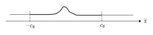
where x ~ ~ 𝑥 \widetilde{x} y ~ ~ 𝑦 \widetilde{y} ∂ H 0 ∂ x ¯ → 0 → subscript 𝐻 0 ¯ 𝑥 0 \dfrac{\partial H_{0}}{\partial\bar{x}}\to 0 ∂ S ∂ x → 0 → 𝑆 𝑥 0 \dfrac{\partial S}{\partial x}\to 0 H 1 → 0 → subscript 𝐻 1 0 H_{1}\to 0 x → ± ∞ → 𝑥 plus-or-minus x\to\pm\infty
From assumption ( ∂ H 0 ∂ y ¯ ) 2 + ( ∂ H 0 ∂ x ¯ ) 2 > const superscript subscript 𝐻 0 ¯ 𝑦 2 superscript subscript 𝐻 0 ¯ 𝑥 2 const \Big{(}\dfrac{\partial H_{0}}{\partial\bar{y}}\Big{)}^{2}+\Big{(}\dfrac{\partial H_{0}}{\partial\bar{x}}\Big{)}^{2}>\mathrm{const} ∂ H 0 ∂ x ¯ → 0 → subscript 𝐻 0 ¯ 𝑥 0 \dfrac{\partial H_{0}}{\partial\bar{x}}\to 0 x ¯ → ± ∞ → ¯ 𝑥 plus-or-minus \bar{x}\to\pm\infty | ∂ H 0 ∂ y ¯ | > const subscript 𝐻 0 ¯ 𝑦 const \left|\dfrac{\partial H_{0}}{\partial\bar{y}}\right|>\mathrm{const} | x ¯ | ¯ 𝑥 |\bar{x}| | x ¯ | > c 6 ¯ 𝑥 subscript 𝑐 6 |\bar{x}|>c_{6} | ∂ H 0 ∂ y ¯ | > c 7 − 1 subscript 𝐻 0 ¯ 𝑦 superscript subscript 𝑐 7 1 \left|\dfrac{\partial H_{0}}{\partial\bar{y}}\right|>c_{7}^{-1} c 6 subscript 𝑐 6 c_{6} c 7 subscript 𝑐 7 c_{7} y ¯ ˙ = d y ¯ d t = − ε ( ∂ H 0 ∂ x ¯ + ε ∂ H 1 ∂ x ¯ ) ˙ ¯ 𝑦 d ¯ 𝑦 d 𝑡 𝜀 subscript 𝐻 0 ¯ 𝑥 𝜀 subscript 𝐻 1 ¯ 𝑥 \dot{\bar{y}}=\dfrac{\mathrm{d}\bar{y}}{\mathrm{d}t}=-\varepsilon\left(\dfrac{\partial H_{0}}{\partial\bar{x}}+\varepsilon\dfrac{\partial H_{1}}{\partial\bar{x}}\right) x ¯ ˙ = d x ¯ d t = ε ( ∂ H 0 ∂ y ¯ + ε ∂ H 1 ∂ y ¯ ) ˙ ¯ 𝑥 d ¯ 𝑥 d 𝑡 𝜀 subscript 𝐻 0 ¯ 𝑦 𝜀 subscript 𝐻 1 ¯ 𝑦 \dot{\bar{x}}=\dfrac{\mathrm{d}\bar{x}}{\mathrm{d}t}=\varepsilon\left(\dfrac{\partial H_{0}}{\partial\bar{y}}+\varepsilon\dfrac{\partial H_{1}}{\partial\bar{y}}\right) H 0 + ε H 1 = const subscript 𝐻 0 𝜀 subscript 𝐻 1 const H_{0}+\varepsilon H_{1}=\mathrm{const} ( x ¯ , y ¯ ) ¯ 𝑥 ¯ 𝑦 (\bar{x},\bar{y}) H 0 = const subscript 𝐻 0 const H_{0}=\mathrm{const} | x ¯ | ≤ c 6 + 1 ¯ 𝑥 subscript 𝑐 6 1 |\bar{x}|\leq c_{6}+1
Figure 14:
Thus for some time moments t + subscript 𝑡 t_{+} t − subscript 𝑡 t_{-}
x ¯ ( t + ) > c 6 , x ¯ ( t − ) < − c 6 . formulae-sequence ¯ 𝑥 subscript 𝑡 subscript 𝑐 6 ¯ 𝑥 subscript 𝑡 subscript 𝑐 6 \bar{x}(t_{+})>c_{6},\quad\bar{x}(t_{-})<-c_{6}.
Then for t > t + 𝑡 subscript 𝑡 t>t_{+}
x ¯ ˙ = ε ( ∂ H 0 ∂ y ¯ + ε ∂ H 1 ∂ y ¯ ) > ε ( c 7 − 1 + O ( ε ) ) > 1 2 ε c 7 − 1 . ˙ ¯ 𝑥 𝜀 subscript 𝐻 0 ¯ 𝑦 𝜀 subscript 𝐻 1 ¯ 𝑦 𝜀 superscript subscript 𝑐 7 1 𝑂 𝜀 1 2 𝜀 superscript subscript 𝑐 7 1 \dot{\bar{x}}=\varepsilon\left(\frac{\partial H_{0}}{\partial\bar{y}}+\varepsilon\frac{\partial H_{1}}{\partial\bar{y}}\right)>\varepsilon\big{(}c_{7}^{-1}+O(\varepsilon)\big{)}>\frac{1}{2}\,\varepsilon\,c_{7}^{-1}.
Therefore, x ¯ ( t ) → + ∞ → ¯ 𝑥 𝑡 \bar{x}(t)\to+\infty t → + ∞ → 𝑡 t\to+\infty x ¯ ( t ) → − ∞ → ¯ 𝑥 𝑡 \bar{x}(t)\to-\infty t → − ∞ → 𝑡 t\to-\infty
From
y = y ¯ + ε ∂ S ( I ¯ , q , y ¯ , x ) ∂ x = y ¯ + ε V ( I ¯ , φ ¯ , y ¯ , x ) , 𝑦 ¯ 𝑦 𝜀 𝑆 ¯ 𝐼 𝑞 ¯ 𝑦 𝑥 𝑥 ¯ 𝑦 𝜀 𝑉 ¯ 𝐼 ¯ 𝜑 ¯ 𝑦 𝑥 y=\bar{y}+\varepsilon\frac{\partial S(\bar{I},q,\bar{y},x)}{\partial x}=\bar{y}+\varepsilon V(\bar{I},\bar{\varphi},\bar{y},x),
taking limiting values on both sides as t → ± ∞ → 𝑡 plus-or-minus t\to\pm\infty y − y ¯ → 0 → 𝑦 ¯ 𝑦 0 y-\bar{y}\to 0
We also know that
p = P ( I , φ , y , x ) = P ( I ¯ , φ ¯ , y ¯ , x ) , 𝑝 𝑃 𝐼 𝜑 𝑦 𝑥 𝑃 ¯ 𝐼 ¯ 𝜑 ¯ 𝑦 𝑥 \displaystyle p=P(I,\varphi,y,x)=P(\bar{I},\bar{\varphi},\bar{y},x),
q = Q ( I , φ , y , x ) = Q ( I ¯ , φ ¯ , y ¯ , x ) . 𝑞 𝑄 𝐼 𝜑 𝑦 𝑥 𝑄 ¯ 𝐼 ¯ 𝜑 ¯ 𝑦 𝑥 \displaystyle q=Q(I,\varphi,y,x)=Q(\bar{I},\bar{\varphi},\bar{y},x).
As y − y ¯ → 0 → 𝑦 ¯ 𝑦 0 y-\bar{y}\to 0 I − I ¯ → 0 → 𝐼 ¯ 𝐼 0 I-\bar{I}\to 0 φ − φ ¯ → 0 → 𝜑 ¯ 𝜑 0 \varphi-\bar{\varphi}\to 0 t → ± ∞ → 𝑡 plus-or-minus t\to\pm\infty
Therefore,
lim t → ± ∞ I ( t ) = lim t → ± ∞ I ¯ ( t ) . subscript → 𝑡 plus-or-minus 𝐼 𝑡 subscript → 𝑡 plus-or-minus ¯ 𝐼 𝑡 \lim\limits_{t\to\pm\infty}I(t)=\lim\limits_{t\to\pm\infty}\bar{I}(t).
Thus I 𝐼 I I ¯ ¯ 𝐼 \bar{I} Δ I = Δ I ¯ Δ 𝐼 Δ ¯ 𝐼 \Delta I=\Delta\bar{I}
Corollary 5.2 .
The estimate
Δ I = O ( e − γ ε ) Δ 𝐼 𝑂 superscript e 𝛾 𝜀 \Delta I=O(\mathrm{e}^{-\frac{\gamma}{\varepsilon}})
is valid.