Atomic states in optical traps near a planar surface

Abstract

In this work we discuss the atomic states in a vertical optical lattice in proximity of a surface. We study the modifications to the ordinary Wannier-Stark states in presence of a surface and we characterize the energy shifts produced by the Casimir-Polder interaction between atom and mirror. In this context, we introduce an effective model describing the finite size of the atom in order to regularize the energy corrections. In addition, the modifications to the energy levels due to a hypothetical non-Newtonian gravitational potential as well as their experimental observability are investigated.

I Introduction

Atomic interferometry has the potential to become a powerful method to investigate atom-surface interactions, the main reason being the high precision which can be reached in frequency measurements. In this context a new experiment named FORCA-G (FORce de CAsimir et Gravitation à courte distance) has been recently proposed WolfPRA07 . The purpose of this experiment is manifold: on one hand it aims at providing a new observation of the Casimir-Polder interaction between an atom and a surface, resulting from the coupling of the fluctuating quantum electromagnetic field with the atom ScheelActaPhysSlov08 ; on the other hand it also intends to impose new constraints on the existence of hypothetical deviations from the Newtonian law of gravitation. These goals will be achieved thanks to the innovative design of FORCA-G, in which interferometric techniques are combined with a trapping potential. This is generated by a vertical standing optical wave produced by the reflection of a laser on a mirror. The vertical configuration leads to an external potential on the atom given by the sum of the optical one and a linear gravitational term due to the earth: this deviation from a purely periodical potential produces a localization of the atomic wavepacket, corresponding to the transition from Bloch to Wannier-Stark states GluckPhysRep02 . The main advantages of FORCA-G are thus the refined control of the atomic position as well as the high precision of interferometric measurements, as demonstrated in the first experimental results BeaufilsArxiv .

Having in mind a theory-experiment comparison within a given accuracy, the theoretical treatment of the problem as well as the experimental investigation must be independently assessed with the same precision. In the case of FORCA-G this demands a detailed theoretical study of the atomic wavefunctions and energy levels in proximity of a surface. As an intermediate step, a precise characterization of the Casimir-Polder atom-surface interaction is also needed.

These issues are the main subject of investigation of this paper. As a matter of fact, the influence of the Casimir-Polder interaction on the atomic energy levels has so far been explored WolfPRA07 ; DereviankoPRL09 using the simple idea of calculating the electrodynamical potential at the center of each well of the trap. We will discuss the validity of this model focusing in particular on the scheme of FORCA-G. In this work, we present a hamiltonian approach to this problem. This treatment first allows us to discuss, independently on the Casimir-Polder atom-surface interaction, the atomic trapped states. Since the presence of the surface breaks the translational symmetry typical of Bloch and Wannier-Stark problems, we focus in particular on the difference (both in energy levels and wavefunctions) between our trapped states and the standard Wannier-Stark solutions. Then, in order to discuss the Casimir-Polder corrections to the energy levels, we generalize the perturbative treatment usually exploited to deduce atom-surface electrodynamical interactions, by including the external optical and gravitational potentials, and treating as a consequence the atomic coordinate as a dynamic variable. The theoretical work presented here will be useful for all experiments that aim at measuring short range interactions between atoms trapped in optical lattices and a macroscopic surface WolfPRA07 ; DereviankoPRL09 ; SorrentinoPRA09 as they will require precise modelling of the atomic states and energy levels close to the surface.

This paper is organized as follows. In section II we describe our physical system. Then, in section III we discuss the shape of atomic wavefunctions in the trap. Section IV is dedicated to the study of the Casimir-Polder interaction and its influence on the atomic energy levels. In this section we introduce an effective description of the finite size of the atom and discuss its validity in connection with the experiment. In section V we look at the energy shifts introduced by a hypothetical non-Newtonian potential and we investigate the constraints that FORCA-G could impose on the strength of this deviation. Finally, in section VI we discuss our results.

II The physical system

In this section we are going to describe the main features of our physical system and the hamiltonian formalism used to investigate the interaction between atom and electromagnetic field. Let us consider a two-level atom trapped in an optical standing wave produced by the reflection of a laser having wavelength $\lambda_{l}=\frac{2\pi}{k_{l}}$ on a surface located at $z=0$. In the configuration we are considering the optical trap has a vertical orientation, so that we have to take into account the earth’s gravitation field acting on the atom. The complete hamiltonian can be written under the form

$$\begin{split}H&=H_{0}+H_{\text{int}}=H_{\text{f}}+H_{\text{at}}+H_{\footnotesize\text{WS}}+H_{\text{int}}\\ H_{\text{f}}&=\sum_{p}\int_{0}^{+\infty}dk_{z}\int d^{2}\mathbf{k}\,\hbar\omega\,a^{\dagger}_{p}(\mathbf{k},k_{z})a_{p}(\mathbf{k},k_{z})\\ H_{\text{at}}&=\hbar\omega_{0}\displaystyle{|e\rangle}\displaystyle{\langle e|}\\ H_{\footnotesize\text{WS}}&=\frac{p^{2}}{2m}+mgz+\frac{U}{2}\bigl{(}1-\cos(2k_{l}z)\bigr{)}\\ H_{\text{int}}&=-\mbox{\boldmath$\mu$}\cdot\mathbf{\mathcal{E}}(\mathbf{r}).\end{split}$$ (1)

The complete Hamiltonian is written as a sum of a term $H_{0}$ describing the free evolution of the atomic and field degrees of freedom. In particular, $H_{\text{f}}$ is the Hamiltonian of the quantum electromagnetic field, described by a set of modes $(p,\mathbf{k},k_{z})$: here $p$ is the polarization index, taking the values $p=1,2$ corresponding to TE and TM polarization respectively, while $\mathbf{k}$ and $k_{z}$ are the transverse and longitudinal components of the wavevector. We associate to each single mode a frequency $\omega=c\sqrt{k^{2}+k_{z}^{2}}$, as well as annihilation and a creation operators $a_{p}(\mathbf{k},k_{z})$ and $a^{\dagger}_{p}(\mathbf{k},k_{z})$. An eigenstate of the field Hamiltonian is thus specified by giving a set of photon occupation numbers $\displaystyle{|\{n_{p}(\mathbf{k},k_{z})\}\rangle}$ for each mode of the field. The vacuum state of the field, with zero photons in each mode, will be noted with $\displaystyle{|0_{p}(\mathbf{k},k_{z})\rangle}$. In our formalism the expression of the electric field is the following

$$\begin{split}\mathbf{\mathcal{E}}(\mathbf{r})&=\frac{i}{\pi}\sum_{p}\int_{0}^{+\infty}dk_{z}\int d^{2}\mathbf{k}\sqrt{\frac{\hbar\omega}{4\pi\epsilon_{0}}}\\ &\,\times\bigl{(}e^{i\mathbf{k}\cdot\mathbf{r}_{\perp}}\mathbf{f}_{p}(\mathbf{k},k_{z},z)a_{p}(\mathbf{k},k_{z})-\text{h.c.}\bigr{)}\end{split}$$ (2)

where we have introduced the transverse coordinate $\mathbf{r}_{\perp}=(x,y)$ and the mode functions $\mathbf{f}_{p}(\mathbf{k},k_{z},z)$ characterizing the boundary conditions imposed on the field. Under the assumption of a perfectly conducting mirror in $z=0$ these functions take a very simple expression BartonJPhysB74

$$\begin{split}\mathbf{f}_{1}(\mathbf{k},k_{z},z)&=\hat{\mathbf{k}}\times\hat{\mathbf{z}}\sin(k_{z}z)\\ \mathbf{f}_{2}(\mathbf{k},k_{z},z)&=\hat{\mathbf{k}}\frac{ick_{z}}{\omega}\sin(k_{z}z)-\hat{\mathbf{z}}\frac{ck}{\omega}\cos(k_{z}z)\end{split}$$ (3)

where $\hat{\mathbf{k}}=\mathbf{k}/k$ and $\hat{\mathbf{z}}=(0,0,1)$. $H_{\text{at}}$ is the internal Hamiltonian of our two level atom having ground state $\displaystyle{|g\rangle}$ and excited state $\displaystyle{|e\rangle}$ separated by a transition frequency $\omega_{0}$. While $H_{\text{at}}$ is associated to the internal atomic degrees of freedom, the term $H_{\footnotesize\text{WS}}$ accounts for the external atomic dynamics. As a consequence, it contains the kinetic energy ($p$ being the canonical momentum associated to $z$), as well as both the gravitational potential (treated here in first approximation as a linear term), where $m$ is the atomic mass and $g$ is the acceleration of the Earth’s gravity, and the classical description of the stationary optical trap, having depth $U$. We treat here only the $z$-dependent terms of the Hamiltonian since the degrees of freedom $x$ and $y$, even in presence of a transverse trapping mechanism, are decoupled from the longitudinal dynamics. For simplicity, we shall take as a unit of energy the photon recoil energy $E_{r}$ given by $E_{r}=\frac{\hbar^{2}k_{l}^{2}}{2m}$. As far as the atomic position is concerned, it will be expressed in units of the periodicity of the trap $\frac{\lambda_{l}}{2}$. For all numerical examples in this paper we will use the experimental configuration chosen for FORCA-G: $E_{r}=5.37\times 10^{-30}\,$J ($\frac{E_{r}}{h}=8.11\times 10^{3}\,$Hz) and $\frac{\lambda_{l}}{2}=266\,$nm.

The interaction between the atom and the quantum electromagnetic field is written here in the well-known multipolar coupling in dipole approximation PowerPhilTransRoySocA59 , where $\mbox{\boldmath$\mu$}=q\mbox{\boldmath$\rho$}$ ($q$ being the electron’s charge and $\rho$ the internal atomic coordinate) is the quantum operator associated to the atomic electric dipole moment and the electric field is calculated in the atomic position $\mathbf{r}$. It is important to observe that, since $\mu$ clearly operates only on the atomic internal states, this interaction term is the only one coupling atomic (both internal and external) and field degrees of freedom. As a consequence, the ground state of the free Hamiltonian $H_{0}$ is simply given by the tensor product of the vacuum field state $\displaystyle{|0_{p}(\mathbf{k},k_{z})\rangle}$, the atomic state $\displaystyle{|g\rangle}$ and the ground state of $H_{\footnotesize\text{WS}}$. In the picture of atomic dressing CPP95 , the ground state of $H_{0}$ is the bare ground state, and the inclusion of $H_{\text{int}}$ will produce a new ground state of the complete system, referred to as dressed ground state, mixing all the degrees of freedom. We are going to tackle the calculation of the ground state of $H_{\footnotesize\text{WS}}$ in the next section, whereas the atom-field interaction will be treated in section IV.

III Modified Wannier-Stark states

III.1 Ordinary Wannier-Stark states

In solid state physics, it is well-known that the solution of the time-independent Schrödinger equation describing a quantum particle in a periodic potential leads to the so-called Bloch states BlochZPhys29 ; Ashcroft . Due to the periodicity of the system, these states are completely delocalized in space coordinate and the spectrum energy is composed of bands of permitted energies, each band being labeled with an index $b=1,2,\dots$. The addition of a linear potential (whose role is in our case played by gravity) to the trap produces localization of the states: these states are usually labeled as Wannier-Stark states (see e.g. WannierPhysRev60 ; GluckEurJPhysD98 ). We will now describe their main features. For each Bloch band $b$, a discrete quantum number $n$ is introduced, taking the values $n=0,\pm 1,\pm 2,\dots$. The state $\displaystyle{|n,b\rangle}^{\text{\tiny{(WS)}}}$ is, in coordinate representation, approximately centered in the $n$-th well of the optical trap, and the energy of this state is in first approximation given by

$$E^{\text{\tiny{(WS)}}}_{n,b}=\bar{E}^{\text{\tiny{(WS)}}}_{b}+n\frac{mg\lambda_{l}}{2E_{r}}$$ (4)

with $\bar{E}^{\text{\tiny{(WS)}}}_{b}$ the average of the $b$-th Bloch band NiuPRL96 ; GluckPhysRep02 . As a result of the quasi-periodicity of the system (i.e. of the linearity of the gravitational potential modifying the periodic trap) two states $\displaystyle{|n,b\rangle}^{\text{\tiny{(WS)}}}$ and $\displaystyle{|p,b\rangle}^{\text{\tiny{(WS)}}}$ belonging to the same band $b$ are shifted, in coordinate representation, by $n-p$ wells. At the same time their energies differ, in accordance with eq. (4), by $n-p$ times $\delta_{g}=\frac{mg\lambda_{l}}{2E_{r}}$. Then, the problem of Wannier-Stark states is solved once we know, for each band $b$, the average Bloch-band energy $\bar{E}^{\text{\tiny{(WS)}}}_{b}$ and the eigenfunction centered in a given well. The Wannier-Stark states can be calculated using, for example, the numerical approach of GluckEurJPhysD98 .

In figures 1 and 2 we give the Wannier-Stark states $\displaystyle{|0,1\rangle}^{\text{\tiny{(WS)}}}$ for two different values of the potential depth $U=3,10$ (in units of $E_{r}$).

Figure 1: Coordinate representation of the state $\displaystyle{|0,1\rangle}$ belonging to the first Bloch band and centered in the zeroth well for $U=3$.

Figure 2: Coordinate representation of the state $\displaystyle{|0,1\rangle}$ belonging to the first Bloch band and centered in the zeroth well for $U=10$.

The figures show that, as expected, a deeper well produces a more localized state of the particle.

III.2 Wannier-Stark states in proximity of a surface

In the context of our problem, the presence of a surface at $z=0$ plays two roles. On one hand, it induces a modification of the Wannier-Stark states by imposing a boundary condition on the eigenvalue problem. On the other hand, the quantum electrodynamical interaction between the atom and this surface must be taken into account, as we will describe in section IV.

The surface at $z=0$ breaks the quasi-periodicity of the system. The potential modifying the optical trap is no longer linear, since it must be considered as the gravitational linear potential for $z>0$ and an infinite potential barrier for $z\leq 0$, describing the impossibility of the particle to penetrate into the mirror. We will refer to the eigenstates of this new physical system as the modified Wannier-Stark states. From now on we are going to deal only with these new states: the state of the $b$-th Bloch band centered in the $n$-th well will be noted with $\displaystyle{|n,b\rangle}$ (and correspondingly $\psi_{n,b}(z)$).

We have solved the problem of modified Wannier-Stark states numerically, using a finite-difference method. The first step of our approach consists in considering a unidimensional box $0<z<z_{f}$ and imposing that the wavefunction vanishes at the borders. As for $z=0$, this corresponds to a real physical boundary condition, whereas the condition $\psi(z_{f})=0$ is purely numerical. Naturally, the acceptability of the solutions will depend on their rate of decay toward 0 for $z\to z_{f}$. The next step is the discretization of the interval $[0,z_{f}]$ using a set of $N+2$ mesh points $z_{i}$ with $z_{0}=0,z_{1},\dots,z_{N+1}=z_{f}$ (giving $\delta z=\frac{z_{f}}{N+1}$ for equally spaced mesh points).

Using this approach, the problem is reduced to an eigenvalue problem of a tridiagonal symmetric matrix. The solution of such a problem can be efficiently worked out using the numerical approach first introduced in PetersTheComputerJournal69 as well as a standard QL algorithm Press95 . In order to check the robustness of our numerical results, we have also checked their coherence with a finite-element method AbrashkevichCompPhysComm95 ; SukumarIntJNumerMethEngng09 .

Choosing a large enough numerical box, taking for example $z_{f}=30$ (we recall here that $z$ is measured in units of trap periods $\frac{\lambda_{l}}{2}$), we have verified that the modified Wannier-Stark states centered in a well far from the surface (approximately starting from $n=10$) have the same shape as the functions shown in section III.1: this reflects the fact that far from the surface the quasi-periodicity of the system is reestablished. Moreover, in this region we find that the energy difference between two successive states equals the expected quantity $\delta_{g}$ defined before: starting from $n=10$, the differences equal $\delta_{g}$ with a relative precision better than $10^{-4}$. This can be seen in table 1, where we show the results obtained for the first ten energy levels with $U=3$: in this table we give the energy levels $E_{n}$, as well as the differences $\delta E_{n}=E_{n+1}-E_{n}$. In this configuration we have $\delta_{g}=0.070068$.

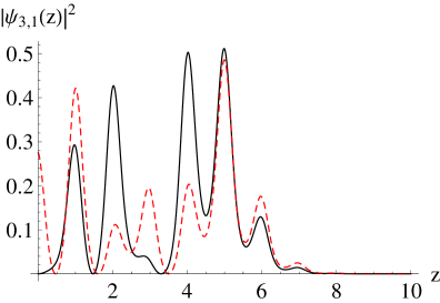
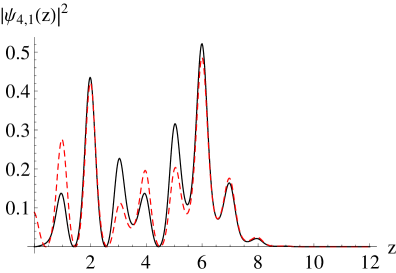
Figure 3: (Color online) Density probability of modified Wannier-Stark states $\psi_{n,1}(z)$ for $n=1,2,3,4$ and $U=3$. The last two functions (black, solid line) are compared to the corresponding standard Wannier-Stark state (red, dashed line).

Table 1 shows only values of the energies belonging to the first Bloch band ($b=1$). We have checked that, increasing the value of $N$ above $10^{6}$, the last digit reported in table 1 remains constant, corresponding to a relative precision of approximately $10^{-4}$. Actually, as a result of our numerical method we also found the eigenvalues and corresponding states associated to higher bands. Nevertheless, we shall discuss only the first-band states since the ones belonging to higher bands are much less relevant for experimental purposes: as a matter of fact, higher bands are not efficiently trapped in the experiment (the average energy of the second band is around $4E_{r}$ for a trap depth of $3E_{r}$).

$n$	$E_{n}$	$\delta E_{n}(\times 10^{-2})$	$\delta E_{n}(\times 10^{2}\text{Hz})$
1	1.4028	12.302	9.9788
2	1.5258	9.8043	7.9525
3	1.6239	8.4432	6.8485
4	1.7083	7.6206	6.1812
5	1.7845	7.2026	5.8422
6	1.8566	7.0518	5.7199
7	1.9271	7.0146	5.6897
8	1.9972	7.0079	5.6843
9	2.0673	7.0070	5.6835
10	2.1374	7.0068	5.6834
11	2.2074	7.0068	5.6834
12	2.2775	7.0068	5.6834
13	2.3476	7.0068	5.6834

Table 1: First ten values of the modified Wannier-Stark spectrum for $U=3$. These values have been obtained on an interval $[0,30]$. The first two columns are in units of $E_{r}$, the third one is in Hz.

As far as the states in proximity of the plate are concerned, they are strongly modified by the boundary condition, and the same property holds for their energies. We show, in figure 3 the first four eigenfunctions in presence of the surface. For the sake of comparison, the third and fourth wavefunctions are superposed to the standard Wannier-Stark solutions centered in the corresponding well. It is important to stress that the ordinary Wannier-Stark functions of wells $n=3,4$ are plotted only to show that the shape of the modified ones tends towards the standard solution: however, the fact that the ordinary functions for these wells are different from zero for $z\leq 0$ makes strictly speaking no sense for our physical system.

In order to discuss the influence of the depth of the wells, we will conclude this section giving the results obtained for $U=10$. In this case, since the ordinary Wannier-Stark states are much more localized in each well, we expect the influence of the surface to be evident on a smaller range of distances. This can be seen directly from table 2, where the energy differences converge more rapidly to $\delta_{g}$.

$n$	$E_{n}$	$\delta E_{n}(\times 10^{-2})$	$\delta E_{n}(\times 10^{2}\text{Hz})$
1	2.9496	7.5127	6.0938
2	3.0247	7.0276	5.7003
3	3.0950	7.0072	5.6837
4	3.1651	7.0068	5.6834
5	3.2352	7.0068	5.6834
6	3.3052	7.0068	5.6834
7	3.3753	7.0068	5.6834
8	3.4454	7.0068	5.6834
9	3.5154	7.0068	5.6834
10	3.5855	7.0068	5.6834

Table 2: First ten values of the modified Wannier-Stark spectrum for $U=10$. Same parameters as for table 1.

Moreover, from figure 4 we see that the state $\psi_{2,1}(z)$ shows already a remarkable accordance with the corresponding unmodified Wannier-Stark state in the interval $[0.6,6]$, where the probability of finding the atom is approximately $0.9997$.

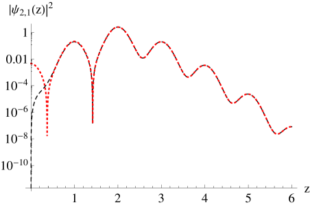
Figure 4: (Color online) Density probability of modified Wannier-Stark states $\psi_{2,1}(z)$ (black, dashed line) for $U=10$ compared to the corresponding standard Wannier-Stark state (red, dotted).

IV Casimir-Polder interaction

IV.1 Standard Casimir-Polder calculations

The presence of the surface does not only play the role of imposing a boundary condition on the Wannier-Stark wavefunctions. In fact, since it modifies the structure of the modes of the quantum electromagnetic field, it is source of an attractive force between the atom and the plate. This is a particular case of a general phenomenon usually called Casimir effect for two macroscopic bodies and Casimir-Polder force when it involves one or more atoms near a surface (for a general review see e.g. Milonni ). This phenomenon was first pointed out by Casimir in 1948 for two parallel perfectly conducting plates CasimirProcKonNederlAkadWet48 and in the same year by Casimir and Polder for atom-surface and atom-atom systems CasimirPhysRev48 .

The Casimir-Polder force between an atom and a mirror has been measured quite recently using several different techniques: deflection of atomic beams SukenikPRL93 , reflection of cold atoms LandraginPRL96 ; ShimizuPRL01 ; DruzhininaPRL03 . In the past few years, Bose-Einstein condensates proved to be efficient probes of this effect, both by means of reflection techniques PasquiniPRL04 ; PasquiniPRL06 and observing center-of-mass oscillations of the condensate AntezzaPRA04 ; HarberPRA05 ; AntezzaPRL06 ; ObrechtPRL07 . The FORCA-G experiment aims at achieving a percent precision in the measurement of the force thanks to the combination of cold atoms and interferometric techniques.

From a theoretical point of view, the force is usually obtained from an interaction energy which results from a time-independent perturbative calculation on the matter-field hamiltonian interaction term CPP95 ; ScheelActaPhysSlov08 . In this kind of approach, the position of the atom is usually treated as a fixed parameter and not as a quantum operator. As a consequence, in order to deduce the Casimir-Polder interaction energy between an atom and a perfectly conducting plate, we must neglect the term $H_{\footnotesize\text{WS}}$ in the Hamiltonian of the system (1) and use eq. (2) for the electric field. Choosing the bare ground state $\displaystyle{|0_{p}(\mathbf{k},k_{z})\rangle}\displaystyle{|g\rangle}$ as the unperturbed configuration, the first-order perturbative correction on interaction term $H_{\text{int}}$ is zero, since the atomic electric dipole moment operator is an odd operator and the annihilation and creation operators appearing in the electric field do not connect states with the same number of photons. Moving to second-order, we obtain the $z$-dependent potential energy

$$V^{(2)}_{\text{CP}}(z)=-\sum_{p}\int_{0}^{+\infty}dk_{z}\int d^{2}\mathbf{k}\frac{\bigl{|}A^{(1)}_{p}(\mathbf{k},k_{z},\mathbf{r})\bigr{|}^{2}}{\hbar(\omega+\omega_{0})}.$$ (5)

In this expression we have defined

$$\begin{split}A^{(1)}_{p}(\mathbf{k},k_{z},\mathbf{r})&=\displaystyle{\langle 0_{p}(\mathbf{k},k_{z})|}\displaystyle{\langle g|}H_{\text{int}}\displaystyle{|1_{p}(\mathbf{k},k_{z})\rangle}\displaystyle{|e\rangle}\\ &=-\frac{i}{\pi}\sqrt{\frac{\hbar\omega}{4\pi\epsilon_{0}}}e^{i\mathbf{k}\cdot\mathbf{r}_{\perp}}\mbox{\boldmath$\mu$}\cdot\mathbf{f}_{p}(\mathbf{k},k_{z},z)\end{split}$$ (6)

and we sum over all the possible intermediate states $\displaystyle{|1_{p}(\mathbf{k},k_{z})\rangle}\displaystyle{|e\rangle}$ having one photon in the mode $(p,\mathbf{k},k_{z})$ and the atom in its excited internal state $\displaystyle{|e\rangle}$. Finally, the superscripts $(2)$ and $(1)$ refer to the order with respect to the electric charge contained in $\mu$.

This result holds for a perfectly conducting surface and at zero temperature. However, the generalization to more realistic configurations including the finite conductivity of the plate as well as a temperature $T>0$ is not straightforward in a perturbative approach. This can be worked out using for example the scattering method LambrechtNewJPhys06 ; MessinaPRA09 or the Green-function formalism (see WyliePRA84 ; BuhmannPRA05 and references therein). The resulting potential can be put under the form FootnoteCasimir

$$\begin{split}V_{\text{CP}}^{(2)}(z)&=\frac{2k_{B}T}{c^{2}}\sum_{n=0}^{+\infty}{}^{\prime}\xi_{n}^{2}\frac{\alpha(i\xi_{n})}{4\pi\epsilon_{0}}\int_{0}^{+\infty}dk\,\frac{ke^{-2K_{n}z}}{2K_{n}}\\ &\,\times\Bigl{[}r_{\mathrm{TE}}(k,i\xi_{n})-\Bigl{(}1+\frac{2c^{2}k^{2}}{\xi_{n}^{2}}\Bigr{)}r_{\mathrm{TM}}(k,i\xi_{n})\Bigr{]}.\\ \end{split}$$ (7)

where $\xi_{n}=\frac{2\pi nk_{B}T}{\hbar}$ is the $n$-th Matsubara frequency and the prime on the Matsubara sum indicates that the $n=0$ term is to be taken with half weight. Moreover we have defined $K_{n}=\sqrt{\frac{\xi_{n}^{2}}{c^{2}}+k^{2}}$ and the $r_{p}(k,\omega)$ are the well-known Fresnel coefficients for a planar surface. Finally $\alpha(\omega)$ is the ground-state atomic polarizability, which for a multilevel atom takes the form FootnotePolarizability

$$\alpha(\omega)=\frac{2}{3}\sum_{n}\frac{E_{n0}\mu_{n0}^{2}}{E_{n0}^{2}-\hbar^{2}\omega^{2}}$$ (8)

where $E_{n0}=E_{n}-E_{0}$ is the difference between the energies of the $n$-th atomic level (starting from the first excited state) and of ground state, whereas $\mu_{n0}$ is the matrix element of the electric dipole operator between the same couple of states. Clearly, the conductive properties of the surface material are included in the Fresnel coefficients through the electric permittivity and magnetic susceptibility $\epsilon(\omega)$ and $\mu(\omega)$ respectively. We conclude this section giving the expression of the Casimir-Polder potential for an atom in front of a real surface at zero temperature

$$\begin{split}V_{\text{CP}}^{(2)}(z)&=\frac{\hbar}{\pi c^{2}}\int_{0}^{+\infty}d\xi\,\xi^{2}\frac{\alpha(i\xi)}{4\pi\epsilon_{0}}\int_{0}^{+\infty}dk\,\frac{ke^{-2Kz}}{2K}\\ &\,\times\Bigl{[}r_{\mathrm{TE}}(k,i\xi)-\Bigl{(}1+\frac{2c^{2}k^{2}}{\xi^{2}}\Bigr{)}r_{\mathrm{TM}}(k,i\xi)\Bigr{]}\\ \end{split}$$ (9)

where $K=\sqrt{\frac{\xi^{2}}{c^{2}}+k^{2}}$ and the sum over the Matsubara frequencies is replaced by an integral.

IV.2 Perturbation of modified Wannier-Stark

In the last section we have given the Casimir-Polder potential for an atom having polarizability $\alpha(\omega)$ in front of an arbitrary planar surface and at temperature $T$. It could be natural to think that this $z$-dependent potential should be added to the Wannier-Stark Hamiltonian $H_{\footnotesize\text{WS}}$ in (1) to obtain a new time-independent problem. So one could obtain a new set of energies and wavefunctions taking also into account the quantum electrodynamical part of the problem. In figure 5 we plot this new complete potential (sum of (5) and the ordinary Wannier-Stark potential) for a Rubidium atom in front of a perfectly conducting surface at zero temperature.

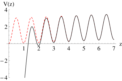
Figure 5: (Color online) Sum of Wannier-Stark (for $U=3$) and Casimir-Polder potentials (in black, solid line) compared to Wannier-Stark potential alone (in red, dashed line).

This plot clearly shows that the Casimir-Polder interaction modifies the optical trap on a limited range. In particular, in our case the first well does no longer exist, the second and the third are slightly modified, and starting from the fourth the trap is practically unperturbed.

Nevertheless, the simple addition of the Casimir-Polder $z$-dependent potential to the external hamiltonian term $H_{\text{WS}}$ is strictly speaking incorrect. As a matter of fact, the potential (5) (as well as (7) and (9)) has been derived using several hypotheses. First, it arises from a perturbative treatment of the interaction term $H_{\text{int}}$ on the Hamiltonian $H_{\text{at}}+H_{\text{f}}$. Moreover, in this calculation the atomic position $z$ is treated as a fixed parameter. This is clearly incoherent with the fact that for our complete Hamiltonian (1) $z$ is a dynamic variable.

These arguments suggest that we should reconsider the calculation of the Casimir-Polder potential using our perturbative approach including the Wannier-Stark Hamiltonian $H_{\footnotesize\text{WS}}$. The perturbative term is still $H_{\text{int}}$, but now the atomic coordinate $z$ has to be treated as a quantum operator as well. So, we are able to introduce a new unperturbed state for each well $n$ of the first Bloch band having the form

$${|\psi^{(0)}_{n,1}\rangle}=\displaystyle{|0_{p}(\mathbf{k},k_{z})\rangle}\displaystyle{|g\rangle}\displaystyle{|n,1\rangle}.$$ (10)

As we found for ordinary Casimir-Polder calculation, the leading-order correction to the energies is the second, and the corrections takes the new form

$$\begin{split}\Delta E^{(2)}_{n,1}&=-\sum_{p}\int_{0}^{+\infty}dk_{z}\int d^{2}\mathbf{k}\\ &\,\times\sum_{p=1}^{+\infty}\sum_{b=1}^{+\infty}\frac{\bigl{|}\displaystyle{\langle\psi^{(0)}_{n,1}|}H_{\text{int}}\displaystyle{|1_{p}(\mathbf{k},k_{z})\rangle}\displaystyle{|e\rangle}\displaystyle{|p,b\rangle}\bigr{|}^{2}}{E^{(0)}_{p,b}-E^{(0)}_{n,1}+\hbar(\omega+\omega_{0})}\end{split}$$ (11)

where now the intermediate state contains the modified Wannier-Stark state $\displaystyle{|p,b\rangle}$. We notice that the difference between two Wannier-Stark energies appearing in the denominator is $p-n$ times approximately $0.07E_{r}$ if the state $\displaystyle{|p,b\rangle}$ belongs to the first band ($b=1$). We now point out that the recoil energy for a Rubidium atom having $m=1.44\cdot 10^{-25}\,$kg trapped in a periodic potential having $\lambda_{l}=532\,$nm is of the order of $10^{-11}\,$eV. On the other hand, the atomic transition energy $\hbar\omega_{0}$ is of the order of the eV. At the same time, the numerator in (11) involves an integral over the $z$ coordinate containing the product of the wavefunctions associated to the two states. This product becomes negligibly small for $|p-n|\gtrsim 7$, whilst the energy difference $E^{(0)}_{p,1}-E^{(0)}_{n,1}$ is still orders of magnitude smaller than $\hbar\omega_{0}$. As a consequence, the Wannier-Stark energy difference in the denominator can be always safely neglected with respect to $\hbar\omega_{0}$ for the intermediate states having $b=1$. As far as the higher bands are concerned, it is possible to see that the same superposition integral decays to zero due to the delocalization of the modified Wannier-Stark states. Furthermore, in the case of higher bands, the energy difference $E^{(0)}_{p,b}-E^{(0)}_{n,1}$ is still $100E_{r}$ (and then still negligible with respect to $\hbar\omega_{0}$) for $b=10$. This reasoning enables us to use the closure relation on the $\displaystyle{|n,b\rangle}$ states and obtain

$$\begin{split}\Delta&E^{(2)}_{n,1}=\\ &\,\displaystyle{\langle n,1|}\Bigl{(}-\sum_{p}\int_{0}^{+\infty}dk_{z}\int d^{2}\mathbf{k}\frac{\bigl{|}A^{(1)}_{p}(\mathbf{k},k_{z},\mathbf{r})\bigr{|}^{2}}{\hbar(\omega+\omega_{0})}\Bigl{)}\displaystyle{|n,1\rangle}.\end{split}$$ (12)

The expression in parentheses coincides with the second-order perturbative calculation on the atom-field ground state described in section IV.1. It is thus evident that the correction we are looking for equals the average on the Wannier-Stark state $\displaystyle{|n,1\rangle}$ of the known Casimir-Polder potential $V_{\text{CP}}^{(2)}(z)$. This can be then expressed as follows

$$\Delta E^{(2)}_{n,1}=\int_{0}^{+\infty}dz\,\bigl{|}\psi^{(0)}_{n,1}(z)\bigr{|}^{2}V^{(2)}_{\text{CP}}(z).$$ (13)

This expression has been obtained in the context of a perturbative treatment for a perfectly conducting surface at zero temperature. Nevertheless, the reasoning which led us from the general expression (11) to the simple average value (13) does not depend on the details of the calculation of the $V^{(2)}_{\text{CP}}(z)$ itself. As a consequence, it is reasonable to assume that the average value (13) can be also used with the more general expressions of the interaction energy (7) or (9).

The behavior of the integrand function around $z=0$ must be treated with care: indeed, the Casimir-Polder potential diverges for $z\to 0$. In particular, it is well-known that for distances much smaller than the typical atomic transition wavelength (van der Waals regime) the interaction potential is temperature-independent and its expression reads AntezzaPRA04

$$V_{\text{CP;vdW}}^{(2)}(z)=-\frac{\hbar}{4\pi z^{3}}\int_{0}^{+\infty}d\xi\,\frac{\alpha(i\xi)}{4\pi\epsilon_{0}}\frac{\epsilon(i\xi)-1}{\epsilon(i\xi)+1}$$ (14)

$\epsilon(\omega)$ being the electric permittivity of the surface material. As for the atomic wavefunction, we have numerically verified that, for any allowed value of $n$, it tends to zero linearly for $z\to 0$. As a consequence, the integrand function behaves like $z^{-1}$ around the origin, implying a divergent energy correction (13) for any $n$. We will develop in the next section an effective description of the atom to regularize this quantity.

IV.3 Regularization of the correction

The potential $V_{\text{CP}}^{(2)}(z)$ represents a particular case of singular potentials since it diverges around the origin faster than $z^{-2}$. The treatment of such potentials has been discussed since the pioneering work of Case CasePhysRev50 (for more details see e.g. FrankRevModPhys71 ). It can be shown from first principles Landau77 that these potentials describe an unphysical situation in proximity of the origin. The solution of the time-independent Schrödinger equation requires in these cases a more detailed knowledge of the short-distance physics of the problem.

In the case of atom-surface interaction, the $z^{-3}$ behavior of the potential is an artefact of treating the atom as a point-like source. This statement is supported by the calculation of the Casimir potential between a sphere of radius $R$ and a wall MaiaNetoPRA08 ; CanaguierPRL09 ; CanaguierArxiv . The potential energy associated with this geometrical configuration shows a $z^{-4}$ long-distance behavior (equivalent to the long-distance Casimir-Polder atom-surface interaction), an intermediate $z^{-3}$ regime and a transition toward a $z^{-1}$ behavior when approaching $z=0$. This property holds for any value of the radius $R$ of the sphere: nevertheless, the characteristic distance at which the transition occurs is, as physically predictable, of the order of the radius.

Inspired by CompagnoEurophysLett88 , we take into account the finite size of the atom by replacing it with a probability density distribution $\rho(\mathbf{r}^{\prime})$. In accordance with CompagnoEurophysLett88 , we make the further assumption that the function $\rho(\mathbf{r}^{\prime})$ is different from zero within a finite volume. Moreover, in our numerical applications, we take this volume to be a sphere of radius $R$, discussing also the dependence of the results on $R$. We assume that the atom has coordinate $(0,0,z)$. We stress here that the atomic coordinate $z$ is taken at the point of the sphere nearest to the surface: as a consequence the effective sphere representing the atom is centered in $(0,0,z+R)$. As far as the probability density distribution is concerned, we will consider the cases of a constant function $\rho_{1}(\mathbf{r}^{\prime})=N_{1}$ and of a spherically symmetric parabolic distribution

$$\rho_{2}(\mathbf{r}^{\prime})=N_{2}\Bigl{[}R^{2}-x^{\prime 2}-y^{\prime 2}-(z^{\prime}-z-R)^{2}\Bigr{]}.$$ (15)

For both probability distributions the variable $\mathbf{r}^{\prime}$ is expressed in the same frame of reference as for the atomic coordinate. The factors $N_{1}$ and $N_{2}$ are to be deduced from the normalization condition

$$\int_{\Omega}d^{3}\mathbf{r}^{\prime}\,\rho(\mathbf{r}^{\prime})=1$$ (16)

being $\Omega$ the spherical atomic volume. Our hypothesis leads to a new regularized expression of the atom-surface potential, given by the average with respect to $\rho(\mathbf{r}^{\prime})$ of the standard Casimir-Polder potential

$$V_{\text{CP;reg}}^{(2)}(z)=\int_{\Omega}d^{3}\mathbf{r^{\prime}}\,\rho(\mathbf{r}^{\prime})V_{\text{CP}}^{(2)}(z^{\prime})$$ (17)

where the $z$-dependence of the new potential is implicitly contained in the probability density distribution $\rho(\mathbf{r}^{\prime})$ and the integration volume $\Omega$. Substituting (17) into (13) then provides the regularized energies of our system.

Let us now analyze the behavior of the regularized potential (17) in proximity of the surface. Assuming that it has a form

$$V_{\text{CP;reg}}^{(2)}(z)=\frac{A}{z^{\alpha}}$$ (18)

the exponent $\alpha$ has the form

$$\alpha=-z\frac{\partial_{z}V_{\text{CP;reg}}^{(2)}(z)}{\partial z}\frac{1}{V_{\text{CP;reg}}^{(2)}(z)}.$$ (19)

In figure 6 we plot the exponent $\alpha$ as a function of $z$ for the standard Casimir-Polder potential (9) and the regularized one (17). Both are calculated in this case for a Rubidium atom in front of a perfectly conducting surface and at zero temperature: the data for the dynamical atomic polarizability of Rubidium were kindly provided by Derevianko et al. DereviankoPRL99 . Furthermore, the regularized expression is calculated for a uniform probability density distribution and three different radii $R=100\,\text{pm},1\,\text{nm},10\,\text{nm}$.

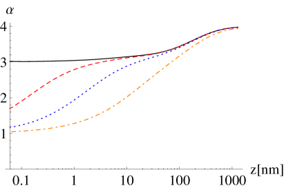
Figure 6: (Color online) Exponent $\alpha$ defined in (19) for the standard Casimir-Polder potential (9) (black, solid line), and the regularized potential (17) for radii 0.1 nm (red, dashed line), 1 nm (blue, dotted line) and 10 nm (orange, dotted-dashed line).

In the four cases it is evident that the transition from $z^{-4}$ to $z^{-3}$ behavior starts around the first atomic transition wavelength ($\simeq 780\,$nm). Moreover, while for the standard Casimir-Polder calculation the exponent tends to 3, in all the other cases the finite size of the atom leads, as anticipated, to a $z^{-1}$ asymptotic dependence. The figure shows clearly that the length scale of this second power-law transition is roughly of the order of the atomic size. We will make use of this regularized potential in the next section to work out the perturbative calculations on the modified Wannier-Stark states.

IV.4 Energy corrections

We are now ready to evaluate the average value (13) of the potential (17) on any modified Wannier-Stark state. Our approach leaves as free parameters the atomic effective radius $R$ and the probability density distribution $\rho(\mathbf{r}^{\prime})$. As far as the radius $R$ is concerned, we first remark that several non-equivalent definitions of the effective atomic radius exist in literature. For example Slater gives in SlaterJChemPhys64 an empirical value of Rubidium radius equal to 235 pm with an associated accuracy of 5 pm. On the contrary, the work ClementiJChemPhys67 estimates the atomic radius for Rubidium to be 265 pm. As a consequence, in order to study the dependence of the results on the value of the radius, we will consider the two extreme cases $R=200\,$pm and $R=300\,$pm. As for the probability distribution, we will use the functions $\rho_{1}(\mathbf{r}^{\prime})$ and $\rho_{2}(\mathbf{r}^{\prime})$ discussed before. Furthermore we are going to consider the case of a perfect conductor for the surface in order to get an insight on the qualitative features of the energy correction. In table 3 we show the energy corrections to the first twelve modified Wannier-Stark states obtained choosing two radii and two probability density distributions. In order to be coherent with the description of the atom as a sphere, the same regularization treatment used for the Casimir-Polder interaction is applied to the other $z$-dependent hamiltonian terms contained in $H_{\text{WS}}$. As expected ($R\ll\lambda_{l}$) this does not modify our results by more than $10^{-3}$ in relative value.

$n$	200 pm - $\rho_{1}$	200 pm - $\rho_{2}$	300 pm - $\rho_{1}$	300 pm - $\rho_{2}$
1	2.39[1]	2.37[1]	2.19[1]	2.16[1]
2	1.76[1]	1.74[1]	1.60[1]	1.58[1]
3	1.20[1]	1.18[1]	1.09[1]	1.08[1]
4	6.80	6.7147	6.18	6.09
5	2.89	2.8557	2.63	2.59
6	8.71[-1]	8.60[-1]	7.91[-1]	7.80[-1]
7	1.93[-1]	1.91[-1]	1.76[-1]	1.74[-1]
8	3.57[-2]	3.53[-2]	3.27[-2]	3.23[-2]
9	6.76[-3]	6.70[-3]	6.33[-3]	6.27[-3]
10	1.84[-3]	1.83[-3]	1.78[-3]	1.78[-3]
11	8.36[-4]	8.35[-4]	8.29[-4]	8.29[-4]
12	5.10[-4]	5.10[-4]	5.09[-4]	5.09[-4]

Table 3: Absolute value (in Hz) of the Casimir-Polder energy corrections (they are all changed in sign) to the first twelve modified Wannier-Stark states for $U=3$. The notation $a[b]$ corresponds to $a\times 10^{b}$. These values are calculated for a perfectly conducting surface.

It is easy to see from table 3 that, as far as the energy levels are concerned, a change in the effective radius produces a more remarkable effect than a change of distribution from the uniform case $\rho_{1}(\mathbf{r}^{\prime})$ to the parabolic $\rho_{2}(\mathbf{r}^{\prime})$. In particular, switching from 200 pm to 300 pm gives a relative error which is of the order of 10% on the first wells and then drops down, whereas the relative correction from $\rho_{1}(\mathbf{r}^{\prime})$ to $\rho_{2}(\mathbf{r}^{\prime})$ is at most around 1%.

It is now instructive to compare one of the set of energy corrections shown in table 3 with the simple evaluation of the strength of the potential energy (9) at the centre of each well WolfPRA07 ; DereviankoPRL09 , which could be used as a first estimation of the energy correction. This idea works better considering deeper traps or farther from the surface: for example, we have verified that the value of $V_{\text{CP}}^{(2)}(z)$ calculated at $z=1$ and the first energy correction differ by a factor of approximately $4.4$ for $U=3$ (see figure 7), while this factors drops already to $1.12$ for $U=20$ and to $1.05$ for $U=80$. We also remark that a larger value of $U$ or a larger atom-surface distance reduces the dependence of the results on the choice of both the probability density distribution and the effective radius. This reasoning proves that in the case of the experiment FORCA-G the delocalization of the atom indeed plays a role.

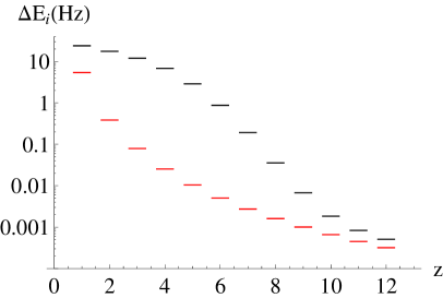
Figure 7: (Color online) Absolute value of the Casimir-Polder energy correction for a uniform distribution and a radius of 200 pm (black upper ticks) compared to the Casimir-Polder potential by evaluating (7) at the well centre (red lower ticks). The depth of the trapping potential is $U=3$.

We want to stress here that the validity of our spherical-atom model used for the regularization of $V_{\text{CP}}^{(2)}(z)$ still remains to be tested by experimental measurements. Some more details, as well as the relationship with the search for non-Newtonian gravity, will be given in section VI.

V Deviations from Newtonian gravitation

Many theories of unification of general relativity and quantum mechanics predict a modification of the laws of gravity at short distances. These modifications can be described by the addition of a new potential to the standard Newtonian one. This correction is often modelized by a Yukawa-type law so that the complete gravitational potential between two point-like particles is written under the form

$$U_{\text{G}}(z)=\frac{GMm}{z}\Bigl{(}1+\alpha_{\footnotesize\text{Y}}e^{-\frac{z}{\lambda_{\footnotesize\text{Y}}}}\Bigr{)}$$ (20)

where $G$ is the gravitational constant, $m$ and $M$ the masses of the two particles. In this expression $\alpha_{\footnotesize\text{Y}}$ and $\lambda_{\footnotesize\text{Y}}$ are two parameters introduced to characterize respectively the relative strength of the corrective potential and its typical range. The experiments aimed at testing the existence of such a deviation set constraints on the allowed values of the parameters $\alpha_{\footnotesize\text{Y}}$ and $\lambda_{\footnotesize\text{Y}}$. The present status of the excluded regions at short ranges ($z<100\,\mu$m) on the $(\alpha_{\footnotesize\text{Y}},\lambda_{\footnotesize\text{Y}})$ plane is depicted in figure 8.

In the experimental configuration of FORCA-G we have verified that the only relevant Yukawa-type contribution is the one associated to the atom-mirror gravitational interaction. At the same time, the Newtonian part of the atom-surface interaction is completely negligible with respect to the Earth-atom term already taken into account in the Wannier-Stark Hamiltonian (1) and with respect to the expected experimental uncertainties. As a consequence, the correction we are looking for is obtained by integrating the Yukawa part of eq. (20) over the volume occupied by the surface. Describing the mirror as a cylinder (the atom being on the direction of its axis) and recalling the we are looking for deviations having length scale $\lambda_{\footnotesize\text{Y}}$ in the $\mu$m range we obtain, after a straightforward calculation,

$$H_{\footnotesize\text{Y}}(z)=2\pi\alpha_{\footnotesize\text{Y}}G\rho_{\footnotesize\text{S}}m\lambda_{\footnotesize\text{Y}}^{2}e^{-\frac{2z}{\lambda_{\footnotesize\text{Y}}}}$$ (21)

$\rho_{\footnotesize\text{S}}$ being the density of the surface. We are now going to find the new unperturbed energy levels of the system (in absence of Casimir-Polder interaction) in presence of the new hamiltonian term (21). This can be done using the method described in section III, after having chosen the value of the parameters $\alpha_{\footnotesize\text{Y}}$, $\lambda_{\footnotesize\text{Y}}$ and $\rho_{\footnotesize\text{S}}$. The new eigenvalues of the unperturbed Hamiltonian $H_{\footnotesize\text{WS}}+H_{\footnotesize\text{Y}}$ will be noted with $E^{\footnotesize\text{(Y)}}_{n}$ for each well $n$. As far as the surface density is concerned, since we still do not have any information about the surface to be used in the experiment, we choose throughout this section just as an example the density of silicon $\rho_{\footnotesize\text{S}}=2.33\times 10^{3}\,\text{kg}\,\text{m}^{-3}$, close to the values corresponding to SiO₂ or BK7 typically used in experiments.

As anticipated in the introduction, one of the the scopes of the experiment FORCA-G is to look for Yukawa-type deviations both near the surface (at distances of the order of $\mu$m) and in the region where the Casimir-Polder interaction can be theoretically modelled at a degree of precision comparable to the experimental noise. In the former regime, the idea of the experiment is to compare the results obtained using two different isotopes of Rubidum (in particular, ⁸⁵Rb and ⁸⁷Rb) in order to make the energy differences between wells almost independent on the Casimir-Polder interaction WolfPRA07 . As a consequence, when discussing the Yukawa correction near the surface, we first need to calculate (both for Wannier-Stark and Yukawa potentials) the differences in energy levels $E_{n}$ and $E^{\footnotesize\text{(Y)}}_{n}$ between ⁸⁵Rb and ⁸⁷Rb, calculated using the formalism described in the previous sections with the different isotope masses in the Hamiltonians (1) and (21). These differences will be noted with.

$$\mathcal{D}E_{n}=\Bigl{(}E^{85}_{n}-E^{87}_{n}\Bigr{)}-\Bigl{(}E^{\footnotesize\text{(Y)}85}_{n}-E^{\footnotesize\text{(Y)}87}_{n}\Bigr{)}$$ (22)

Finally the experiment will be able to detect a Yukawa-type deviation if the difference $\mathcal{D}E_{n}$ is within the experimental sensitivity. In the case of FORCA-G, the expected sensitivity is $10^{-4}\,$Hz WolfPRA07 .

We first give in table 4 the results obtained for $\alpha_{\footnotesize\text{Y}}=3\times 10^{10}$ and $\lambda_{\footnotesize\text{Y}}=1\,\mu$m: the value of $\alpha_{\footnotesize\text{Y}}$ approximately corresponds to the limit of the experimentally accessed region for $\lambda_{\footnotesize\text{Y}}=1\,\mu$m.

$n$	$\mathcal{D}E_{n}$ (Hz)		$n$	$\mathcal{D}E_{n}$ (Hz)
1	1.654[-1]		13	2.0[-3]
2	1.425[-1]		14	1.5[-3]
3	1.221[-1]		15	1.2[-3]
4	9.43[-2]		16	9[-4]
5	5.72[-2]		17	7[-4]
6	2.71[-2]		18	5[-4]
7	1.30[-2]		19	4[-4]
8	8.0[-3]		20	3[-4]
9	6.0[-3]		21	2[-4]
10	4.4[-3]		22	2[-4]
11	3.4[-3]		23	1[-4]
12	2.6[-3]		24	1[-4]

Table 4: First 24 values (the energy differences are expressed in Hz) of the modified Wannier-Stark spectrum for $U=3$ and in presence of the Yukawa-type potential (21) with $\alpha_{\footnotesize\text{Y}}=3\times 10^{10}$ and $\lambda_{\footnotesize\text{Y}}=1\mu\text{m}$.

From these results it is clear that the Yukawa-type deviations corresponding to the couple $(\alpha_{\footnotesize\text{Y}},\lambda_{\footnotesize\text{Y}})$ chosen are, in principle, experimentally detectable up to the well $n=24$ in a differential ⁸⁵Rb – ⁸⁷Rb measurement.

We now turn to the second experimental configuration in which the Casimir-Polder potential is expected to be predicted at the $10^{-4}\,$Hz level WolfPRA07 . We stress that, apart from the precision in the calculation of the non-regularized Casimir-Polder potential, we must pay attention to the uncertainty introduced by our effective description of the finite size of the atom. Assuming that the Casimir-Polder potential can be theoretically determined, independently of its regularization, with at best a $1\%$ accuracy, the absolute precision in its determination can be considered comparable to the experimental error already around the well $n=40$, where $z=10\,\mu$m and the potential equals approximately $0.06\,$Hz, i.e. in this second experimental configuration the atoms will be at 10 $\mu$m or more from the surface. At this distance, our hypothesis of a spherical atom plays already no role. Indeed, we have checked that, using both probability distributions and both radii, the potentials so obtained differ less than $10^{-5}\,$Hz already at $z=5\,\mu$m. This is coherent with the fact that the finite size of the atom plays a negligible role at distances much larger than the atomic size itself. As a consequence, in this second experimental regime the precision on the standard calculation and the experimental uncertainties impose stronger limitations than our effective model.

We have calculated the Yukawa corrections on the well $n=40$ for different values of $\lambda_{\footnotesize{Y}}$: for each of them, we have found our limiting value of $\alpha_{\footnotesize{Y}}$ by looking for a correction of the order of $10^{-4}\,$Hz. We have, moreover, repeated the same calculation for $n=70$ (where $V_{\text{CP}}\simeq 0.01\,$Hz) as well as in the near regime discussed above evaluating the energy difference between wells $n=4$ and $n=6$. These three curves are represented in figure 8 on top of the present experimental constraints.

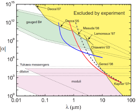
Figure 8: (Color online) In yellow are displayed the regions of the $(\alpha_{\footnotesize\text{Y}},\lambda_{\footnotesize\text{Y}})$ plane excluded by experiments. The figure is taken from GeraciPRL10 . The three superposed curves represent the experimental constraints theoretically calculated for the experiment FORCA-G. They correspond to the near regime, using a superposition between wells $n=4$ and $n=6$ (blue solid line, first from the left), the far regime for $n=40$ (red solid line) and for $n=70$ (black dashed line).

VI Discussion

In this work, we have introduced an effective model describing the atom as a spherical probability distribution. This was needed in order to regularize the expression of the Casimir-Polder energy correction to the modified Wannier-Stark states. It is important to discuss in more detail the validity of this model in connection with the experimental results.

Let us start by recalling that in the context of the search for non-Newtonian gravitation, our model does not impose severe limitations. As a matter of fact, in the near regime the Casimir-Polder contribution is almost cancelled by the use of two isotopes, whereas at far distances we have shown (see sec. V) that the error introduced by our description is negligible with respect to the accuracy in the knowledge of the Casimir-Polder potential itself.

The experiment could be used, in addition, to test the validity of our model. To this aim, measurements should be performed in the near regime (say within the first ten wells) with a single isotope. In this case, the measured energy differences would check the consistency of our atomic description as well as provide an estimation of the effective radius. The use of a single isotope makes the correction coming from the Yukawa potential negligible with respect to the Casimir-Polder term (see tables 3 and 4).

Finally, the experimental setup can be used for a measurement of the Casimir-Polder potential around $5\,\mu$m: in this region, as shown in section V, the energy correction due to the atom-field interaction is almost insensitive to the model chosen and the Yukawa interaction is much smaller than the quantum electrodynamical one. This measure could provide a new experimental observation of the Casimir-Polder potential with a relative uncertainty of less than one part in $10^{3}$.

Nevertheless, we stress here that a precise knowledge of the Casimir-Polder standard potential requires an accurate description of the atomic and surface optical data. The details of the latter are unavailable at present, so the calculation in this paper have performed for perfectly conducting mirror. To complete our analysis it will be enlightening to compare our results to the exact sphere-plate calculations CanaguierPRL09 ; CanaguierArxiv . In this case, as remarked in CanaguierArxiv , an appropriate description of the dielectric properties of the sphere is needed to mimic the atomic optical response.

VII Conclusions

In this paper we have discussed the modifications of the Wannier-Stark states in presence of a surface. As a first step we have considered the presence of the surface as a boundary condition of the time-independent Schrödinger equation obtaining in this way a new class of states. These states, even if asymptotically coincident with the ordinary Wannier-Stark states at large distances from the surface, significantly differ from them, both in energy and shape of the wavefunction, at the first few wells.

We have then also taken into account the Casimir-Polder interaction between the atom and surface as a source of correction to the energy levels of the system. We have shown that these corrections diverge due to the $z^{-3}$ behavior of the electrodynamical potential energy. In order to regularize this result, we have introduced an effective description of the atom as a probability density distributed over a spherical volume. Our description leaves as free parameters both the radius of the sphere and the probability distribution. We have characterized the dependence of our results on both quantities. The validity of this model as well as the values of these parameters remain to be investigated by experiments.

In the second part of the paper we have studied the possibility of measuring a hypothetical Yukawa-type contribution to the gravitational potential at short distances. We have calculated the constraints that the experiment FORCA-G will be able to set on the $(\alpha_{\footnotesize\text{Y}},\lambda_{\footnotesize\text{Y}})$ plane. We have shown that the constraints set by the experiment are dominated by the experimental uncertainties and unaffected (to within those uncertainties) by the choice of the model for the regularization of the CP interaction.

This work paves the way to the precise calculation of the energy levels in the experimental configuration of FORCA-G and other experiments that use atoms in optical dipole traps close to a surface WolfPRA07 ; SorrentinoPRA09 . To this aim, a precise knowledge of the optical data of the mirror and the atom is needed. This information will allow us to give a more detailed estimate of the accuracy of our results, also based on the comparison with independent approaches to the regularization problem. Finally, the knowledge of the atomic wavefunctions constitutes the first ingredient for the description of the dynamics of the system, which is the subject of ongoing work.

- (1) P. Wolf, P. Lemonde, A. Lambrecht, S. Bize, A. Landragin, and A. Clairon, Phys. Rev. A 75, 063608 (2007).
- (2) S. Scheel and S. Y. Buhmann, Acta Phys. Slov. 58, 675 (2008).
- (3) M. Gluck, A. R. Kolovsky, and H. J. Korsch, Phys. Rep. 366, 103 (2002).
- (4) Q. Beaufils, G. Tackmann, B. Pelle, S. Pelisson, P. Wolf, F. Pereira dos Santos, preprint arXiv:1102.5326 (2011).
- (5) A. Derevianko, B. Obreshkov, and V. A. Dzuba, Phys. Rev. Lett. 103, 133201 (2009).
- (6) F. Sorrentino, A. Alberti, G. Ferrari, V. V. Ivanov, N. Poli, M. Schioppo, and G. M. Tino, Phys. Rev. A 79, 013409 (2009).
- (7) G. Barton, J. Phys. B 7, 2134 (1974).
- (8) E. A. Power and S. Zineau, Phil. Trans. Roy. Soc. A 251, 427 (1959).
- (9) G. Compagno, R. Passante, and F. Persico, Atom-Field Interactions and Dressed Atoms (Cambridge University Press, Cambridge, 1995).
- (10) F. Bloch, Z. Phys. 52, 555 (1929).
- (11) N. W. Ashcroft and N. D. Mermin, Solid State Physics (Holt, Rinehan and Winston, New York, 1976).
- (12) G. H. Wannier, Phys. Rev. 117, 1366 (1960).
- (13) M. Gluck, A. R. Kolovsky, H. J. Korsch, and N. Moiseyev, Eur. Phys. J. D 4, 239 (1998).
- (14) Q. Niu, X.-G. Zhao, G. A. Georgakis, and M. G. Raizen, Phys. Rev. Lett. 76, 4504 (1996).
- (15) G. Peters and J. H. Wilkinson, The Computer Journal 12, 398 (1969).
- (16) W. H. Press, S. A. Teukolsky, W. T. Vetterling, and B. P. Flannery, Numerical Recipes in C: The Art of Scientific Computing (Cambridge University Press, Cambridge, 1992).
- (17) A. G. Abrashkevich, D. G. Abrashkevich, M. S. Kaschiev, I. V. Puzynin, Comp. Phys. Comm. 85, 40 (1995).
- (18) N. Sukumar and J. E. Pask, Int. J. Numer. Meth. Engng 77, 1121 (2009).
- (19) P. W. Milonni, The Quantum Vacuum: An Introduction to Quantum Electrodynamics (Academic Press, San Diego, 1994).
- (20) H. B. G. Casimir, Proc. K. Ned. Akad. Wet. Ser. B 51, 793 (1948).
- (21) H. B. G. Casimir and D. Polder, Phys. Rev. 73, 360 (1948).
- (22) C. I. Sukenik, M. G. Boshier, D. Cho, V. Sandoghdar, and E. A. Hinds, Phys. Rev. Lett. 70, 560 (1993).
- (23) A. Landragin, J. Y. Courtois, G. Labeyrie, N. Vansteenkiste, C. I. Westbrook, and A. Aspect, Phys. Rev. Lett. 77, 1464 (1996).
- (24) F. Shimizu, Phys. Rev. Lett. 86, 987 (2001).
- (25) V. Druzhinina and M. DeKieviet, Phys. Rev. Lett. 91, 193202 (2003).
- (26) T. A. Pasquini, Y. Shin, C. Sanner, M. Saba, A. Schirotzek, D. E. Pritchard, and W. Ketterle, Phys. Rev. Lett. 93, 223201 (2004).
- (27) T. A. Pasquini, M. Saba, G. Jo, Y. Shin, W. Ketterle, D. E. Pritchard, T. A. Savas, and N. Mulders, Phys. Rev. Lett. 97, 093201 (2006).
- (28) M. Antezza, L. P. Pitaevskii, and S. Stringari, Phys. Rev. A 70, 053619 (2004).
- (29) D. M. Harber, J. M. Obrecht, J. M. McGuirk, and E. A. Cornell, Phys. Rev. A 72, 033610 (2005).
- (30) M. Antezza, L. P. Pitaevskii, S. Stringari, and V. B. Svetovoy, Phys. Rev. Lett. 97, 223203 (2006).
- (31) J. M. Obrecht, R. J. Wild, M. Antezza, L. P. Pitaevskii, S. Stringari, and E. A. Cornell, Phys. Rev. Lett. 98, 063201 (2007).
- (32) A. Lambrecht, P. A. Maia Neto and S. Reynaud, New J. Phys. 8, 243 (2006).
- (33) R. Messina, D. A. R. Dalvit, P. A. Maia Neto, A. Lambrecht, and S. Reynaud, Phys. Rev. A 80, 022119 (2009).
- (34) J. M. Wylie and J. E. Sipe, Phys. Rev. A 30, 1185 (1984).
- (35) S. Y. Buhmann, D.-G. Welsch and T. Kampf, Phys. Rev. A 72, 032112 (2005).
- (36) The Casimir-Polder potential is naturally expressed, as a result of a perturbative calculation, as an integral over the real axis of frequencies (see e.g. eq. (5)). In order to make calculations easier, a rotation to the imaginary axis is usually performed ScheelActaPhysSlov08 . In the case of zero temperature, since the integrand function has no poles on both axes, the result is an integral over imaginary frequencies (9). On the contrary, the integrand function in the case of non-zero temperature has an infinite number of poles on the imaginary axis, namely the Mastubara frequencies . This explains the sum over appearing in eq. (7).
- (37) It may be useful to specify that the polarizability defined in eq. (8) is given in SI units and has the dimensions of C m2 V-1. The corresponding expression in cgs units is given by and has the dimensions of a volume.
- (38) K. M. Case, Phys. Rev. 80, 797 (1950).
- (39) W. M. Frank, D. J. Land, and R. M. Spector, Rev. Mod. Phys. 43, 36 (1971).
- (40) L. D. Landau, L. P. Pitaevskii, and E.M. Lifshitz, Quantum Mechanics (Pergamon Press, Oxford, 1977).
- (41) P. A. Maia Neto, A. Lambrecht, and S. Reynaud, Phys. Rev. A 78, 012115 (2008).
- (42) A. Canaguier-Durand, P. A. Maia Neto, I. Cavero-Pelaez, A. Lambrecht, and S. Reynaud, Phys. Rev. Lett 102, 230404 (2009).
- (43) A. Canaguier-Durand, and S. Reynaud, preprint arXiv:1101.5258v1 (2011).
- (44) G. Compagno, R. Passante, and F. Persico, Europhys. Lett. 7, 399 (1988).
- (45) A. Derevianko, W. R. Johnson, M. S. Safronova, and J. F. Babb, Phys. Rev. Lett. 82, 3589 (1999).
- (46) J. C. Slater, J. Chem. Phys. 41, 3199 (1964).
- (47) E. Clementi, D. L. Raimondi, and W. P. Reinhardt, J. Chem. Phys. 47, 1300 (1967).
- (48) A. A. Geraci, S. B. Papp, and J. Kitching, Phys. Rev. Lett. 105, 101101 (2010).