Symplectic integrators in the shearing sheet

Abstract

The shearing sheet is a model dynamical system that is used to study the small-scale dynamics of astrophysical disks. Numerical simulations of particle trajectories in the shearing sheet usually employ the leapfrog integrator, but this integrator performs poorly because of velocity-dependent (Coriolis) forces. We describe two new integrators for this purpose; both are symplectic, time-reversible and second-order accurate, and can easily be generalized to higher orders. Moreover, both integrators are exact when there are no small-scale forces such as mutual gravitational forces between disk particles. In numerical experiments these integrators have errors that are often several orders of magnitude smaller than competing methods. The first of our new integrators (SEI) is well-suited for disks in which the typical inter-particle separation is large compared to the particles’ Hill radii (e.g., planetary rings), and the second (SEKI) is designed for disks in which the particles are on bound orbits or the separation is smaller than the Hill radius (e.g., irregular satellites of the giant planets).

1 Introduction

Hill’s approximation, or the shearing sheet approximation, is an essential tool for the study of the small-scale dynamics of astrophysical disks (for a general review of Hill’s approximation see, e.g., Binney & Tremaine, 2008). The method was originally devised by Hill (1878) to study the motion of the Moon, and has been applied to galaxy disks (e.g., Goldreich & Lynden-Bell, 1965; Julian & Toomre, 1966; Goldreich & Tremaine, 1978), accretion disks (e.g., Hawley & Balbus, 1992; Stone & Gardiner, 2010), planetary rings (e.g., Wisdom & Tremaine, 1988; Salo, 1992; Richardson, 1994; Crida et al., 2010; Rein & Papaloizou, 2010) and planetesimal disks (e.g., Tanga et al., 2004; Johansen et al., 2009; Bai & Stone, 2010; Rein et al., 2010). Hill’s approximation is widely used in numerical simulations when it is impossible to model an entire disk with adequate numerical resolution.

This paper discusses numerical methods for following orbits in Hill’s approximation. We first describe the relevant equations of motion in Sect. 2. We then review existing integrators in Sect. 3, and describe two new algorithms. In Sect. 4 we compare the convergence and performance of all these integrators. We summarize and discuss several generalizations in Sect. 5.

2 Hill’s approximation

For simplicity we consider mainly the three-body problem, although the results we describe are easy to generalize to other systems such as planetary rings (see Sect. 5). Thus we follow the motion of two nearby small bodies with masses $m_{1}$ and $m_{2}$ in the gravitational field of a large body of mass $M\gg m_{1},m_{2}$ (a more careful version of this derivation is given by Hénon & Petit 1986). The two small bodies follow approximately the same orbit around the large body, and we assume that this mean orbit is circular with semi-major axis $a$. The angular speed of the mean orbit is then $\Omega=[G(M+m)/a^{3}]^{1/2}$ where $m=m_{1}+m_{2}$. Formally, to derive Hill’s equations of motion, one lets $m/M$ shrink to zero while assuming that the mass ratio $m_{1}/m_{2}$ is fixed and the separation between the two small bodies is of order $(m/M)^{1/3}$.

Let us adopt a local right-handed Cartesian coordinate system with its origin at $m_{1}$, rotating uniformly with angular velocity $\Omega$. The unit vector $\mathbf{e}_{x}$ points away from the larger mass $M$, the unit vector $\mathbf{e}_{y}$ points in the direction of motion along the mean orbit, and the unit vector $\mathbf{e}_{z}$ points in the direction of the angular velocity vector of the mean orbit. Hill’s equations of motion for the relative position $\mathbf{r}=\mathbf{r}_{2}-\mathbf{r}_{1}$ are then

$$\mathbf{\ddot{r}}=-2\Omega\;\mathbf{e}_{z}\times\mathbf{\dot{r}}+3\Omega^{2}(\mathbf{r\cdot e}_{x})\,\mathbf{e}_{x}-\Omega^{2}(\mathbf{r\cdot e}_{z})\,\mathbf{e}_{z}+\mathbf{f},$$ (1)

where the force exerted by $m_{1}$ on $m_{2}$ is $\mathbf{f}=-\mbox{\boldmath$\nabla$}\Phi$ with $\Phi(\mathbf{r})=Gm/|\mathbf{r}|$. The Hamiltonian corresponding to these equations of motion is

$$H(\mathbf{r},\mathbf{p}) ={\textstyle{\frac{1}{2}}}\mathbf{p}^{2}+\Omega\left(\mathbf{p}\times\mathbf{r}\right)\cdot\mathbf{e}_{z}+{\textstyle{\frac{1}{2}}}\Omega^{2}\left[\mathbf{r}^{2}-3\left(\mathbf{r}\cdot\mathbf{e}_{x}\right)^{2}\right]+\Phi(\mathbf{r})$$

$$\equiv H_{0}(\mathbf{r},\mathbf{p})+\Phi(\mathbf{r}),$$ (2)

where $\mathbf{p}=\mathbf{\dot{r}}-\Omega\,\mathbf{r}\times\mathbf{e}_{z}$ is the canonical momentum conjugate to $\mathbf{r}$.

Note that when $\mathbf{f}=\mathbf{0}$ the equations of motion (1) are invariant under the shear transformation

$$\mathbf{r}\rightarrow\mathbf{r}+c_{x}\left(\mathbf{e}_{x}-\tfrac{3}{2}\Omega\mathbf{e}_{y}t\right)+c_{y}\mathbf{e}_{y}$$ (3)

for arbitrary constants $c_{x}$ and $c_{y}$. This invariance allows the use of periodic shearing boundary conditions for the study of the local dynamics of disks and is one reason why Hill’s approximation is so useful.

Alternatively, we can work in a non-rotating but accelerated reference frame with origin at $m_{1}$. If the relative position in this frame is $\mathbf{R}=(X,Y,Z)$ and the $(x,y,z)$ and $(X,Y,Z)$ reference frames coincide at $t=0$, then

$$\mathbf{\ddot{R}}=\Omega^{2}\left([\mathbf{r\cdot e}_{x}(t)]\,\mathbf{e}_{x}(t)-\mathbf{R}\right)+\mathbf{f},$$ (4)

with $\mathbf{e}_{x}(t)=\cos(\Omega t)\mathbf{e}_{X}+\sin(\Omega t)\mathbf{e}_{Y}$. The Hamiltonian is

$$H(\mathbf{R},\mathbf{P},t)={\textstyle{\frac{1}{2}}}\mathbf{P}^{2}+{\textstyle{\frac{1}{2}}}\Omega^{2}\left\{\mathbf{R}^{2}-3[\mathbf{R}\cdot\mathbf{e}_{x}(t)]^{2}\right\}+\Phi(\mathbf{R})$$ (5)

where $\Phi(\mathbf{R})=\Phi(\mathbf{r})=-Gm/|\mathbf{r}|$ since $|\mathbf{R}|=|\mathbf{r}|$.

The physical interpretation of Eqs. (1) and (2), and the optimum choice of integrator, depend on the relative size of the terms on the right side. This can be parametrized using the Hill radius, $r_{\text{Hill}}\equiv(\frac{1}{3}{Gm}/{\Omega^{2}})^{1/3}$, which sets the relevant scale in the problem.

• If the mass of the small bodies is negligible ($m\rightarrow 0,r_{\text{Hill}}\rightarrow 0$) their relative motion is simply epicyclic motion, which can be solved exactly (see e.g. Hénon & Petit, 1986; Binney & Tremaine, 2008, or below). If $m$ is sufficiently small, the motion can be regarded as a perturbed epicycle. Quantitatively, this requires that one or more of the first three terms on the right side of Eq. (1) is much larger than $|\mathbf{f}|=Gm/r^{2}$, or

  $$\frac{r}{r_{\text{Hill}}}\gg\mbox{min}\,\left[1,(\Omega r_{\text{Hill}}/v)^{1/2}\right],$$ (6)

  where $v$ is the velocity. One example is a planetary ring with semi-major axis $a$ much less than the Roche limit $a_{R}=2.46[3M/(4\pi\rho_{p})]^{1/3}$; here $M$ is the planet mass, $m_{1}$ and $m_{2}$ are the masses of the ring particles, and $\rho_{p}$ is the ring-particle density. For two particles the separation between them cannot be less than twice their radius, which implies that $r/r_{\text{Hill}}\gtrsim a_{R}/a\gg 1$.

• If the force due to the mutual gravity of the small masses is large, we can interpret the solution to Eq. (1) as a Keplerian orbit perturbed by Coriolis and tidal forces (the terms proportional to $\Omega$ and $\Omega^{2}$ respectively). For a circular orbit of semi-major axis $r$ the ratio of these perturbing forces to the Kepler force $Gm/r^{2}$ is $(r/r_{\text{Hill}})^{3/2}$ and $(r/r_{\text{Hill}})^{3}$ respectively. One example is the irregular satellites of the giant planets of the solar system, which typically have $r/r_{\text{Hill}}\simeq 0.1$–0.5.

3 Integrators

3.1 Leapfrog integrator

Many N-body simulations, in Hill’s approximation and other contexts, use the standard leapfrog integrator (e.g., Springel, 2005; Binney & Tremaine, 2008). However, as we shall show below, leapfrog does not work well in Hill’s approximation because there are velocity-dependent forces. Leapfrog is best suited for integrating equations of motion of the form

$$\mathbf{\ddot{r}}=-\mbox{\boldmath$\nabla$}\Phi(\mathbf{r})$$ (7)

where $\Phi(\mathbf{r})$ is a (in general time-dependent) potential. Note that Eq. (1) can not be written in this form. The Hamiltonian corresponding to Eq. (7) is

$$H(\mathbf{r},\mathbf{p})={\textstyle{\frac{1}{2}}}\mathbf{p}^{2}+\Phi(\mathbf{r})\equiv H_{\text{Kin}}(\mathbf{p})+\Phi(\mathbf{r}).$$ (8)

We assume that we have the position and velocity of a particle at time $t^{n}$, $\mathbf{r}^{n}\equiv\mathbf{r}(t^{n})$ and $\mathbf{v}^{n}\equiv\mathbf{\dot{r}}(t^{n})=\mathbf{p}(t^{n})$. The goal is to approximate the new position and velocity at time $t^{n+1}=t^{n}+\Delta t$. Leapfrog is usually written as a chain of three operators, labeled Kick, Drift, Kick, applied successively:

$$\begin{array}[]{llll}\quad\mathbf{v}^{n+1/2}&=\mathbf{v}^{n}&+\,\frac{1}{2}\Delta t\;\;\mathbf{f}^{n}&\quad\quad\quad\quad\quad\quad\quad\quad\quad\text{Kick}\\ \quad\mathbf{r}^{n+1}&=\mathbf{r}^{n}&+\,\Delta t\,\mathbf{v}^{n+1/2}&\quad\quad\quad\quad\quad\quad\quad\quad\quad\text{Drift}\\ \quad\mathbf{v}^{n+1}&=\mathbf{v}^{n+1/2}&+\,\frac{1}{2}\Delta t\;\;\mathbf{f}^{n+1}&\quad\quad\quad\quad\quad\quad\quad\quad\quad\text{Kick,}\\ \end{array}\hskip 142.26378pt$$ (12)

where $\mathbf{f}^{n}=-\mbox{\boldmath$\nabla$}\Phi(\mathbf{r}^{n})$. The kick operator corresponds to following the trajectory exactly under the influence of the Hamiltonian $\Phi(\mathbf{r})$, the potential energy, and the drift operator corresponds to the Hamiltonian $H_{\text{Kin}}(\mathbf{p})$, the kinetic energy. Thus if we denote the operator for the exact evolution of a trajectory for a time-step $\Delta t$ under an arbitrary Hamiltonian $H$ by $\hat{H}(\Delta t)$, a single leapfrog step is the operator $\hat{H}_{\text{Kin}}(\tfrac{1}{2}\Delta t)\hat{\Phi}(\Delta t)\hat{H}_{\text{Kin}}(\tfrac{1}{2}\Delta t)$. Each of these operators is symplectic since they are governed by a Hamiltonian, which implies that the leapfrog operator is also symplectic (Saha & Tremaine, 1992). Moreover leapfrog is time-reversible and second-order, that is, the error after a single time-step is $O(\Delta t^{3})$.

When leapfrog is used in Hill’s approximation, to integrate the equations of motion governed by Eq. (1) rather than Eq. (7), the additional terms on the right side are added in the kick step, since they change the velocity. Thus we have (partly in component notation, for clarity):

$$\begin{array}[]{llll}\quad v_{x}^{n+1/2}&=&v_{x}^{n}+\frac{1}{2}\Delta t\left(3\Omega^{2}\,x^{n}+2\Omega\,v_{y}^{n}+f_{x}^{n}\right)\\ \quad v_{y}^{n+1/2}&=&v_{y}^{n}+\frac{1}{2}\Delta t\left(-2\Omega\,v_{x}^{n}+f_{y}^{n}\right)&\text{Kick}\\ \quad v_{z}^{n+1/2}&=&v_{z}^{n}+\frac{1}{2}\Delta t\left(-\Omega^{2}\,z^{n}+f_{z}^{n}\right)\\ \\ \quad\mathbf{r}^{n+1}&=&\mathbf{r}^{n}+\Delta t\;\mathbf{v}^{n+1/2}&\hbox{\multirowsetup\text{Drift}}\\ \\ \quad v_{x}^{n+1}&=&v_{x}^{n+1/2}+\frac{1}{2}\Delta t\left(3\Omega^{2}\,x^{n+1}+2\Omega\,v_{y}^{n+1/2}+f_{x}^{n+1}\right)\\ \quad v_{y}^{n+1}&=&v_{y}^{n+1/2}+\frac{1}{2}\Delta t\left(-2\Omega\,v_{x}^{n+1/2}+f_{y}^{n+1}\right)&\text{Kick}\\ \quad v_{z}^{n+1}&=&v_{z}^{n+1/2}+\frac{1}{2}\Delta t\left(-\Omega^{2}\,z^{n+1}+f_{z}^{n+1}\right).\end{array}\hskip 142.26378pt$$ (22)

However, because of the velocity-dependent Coriolis force on the right side, in this form leapfrog loses most of its desirable properties: (i) it is neither symplectic nor time-reversible; (ii) it is only first-order accurate rather than second-order, that is, the error after a single time-step is $O(\Delta t^{2})$; (iii) it leads to secular drifts in quantities that should be conserved.

In principle these difficulties could be avoided by using leapfrog to integrate the equations of motion in the form (4), which have no velocity-dependent forces so leapfrog is symplectic, time-reversible, and second-order. We do not pursue this option because (i) these equations are not invariant under the shear transformation, Eq. (3), which limits their usefulness for the study of disks and rings; (ii) the method described in Sect. 3.5 below is better.

There are schemes for constructing symplectic integrators for arbitrary Hamiltonians, but these are generally implicit and often algebraically complicated, at least for high-order schemes. The first explicit symplectic integrator for trajectories in Hill’s approximation is due to Heggie (2001). However, Heggie’s integrator is not time-reversible and is only first-order; we will not discuss it further because our numerical experiments show that it is not competitive with the integrators described below.

3.2 Modified leapfrog integrator

One can improve the standard leapfrog algorithm by using a predictor step to approximate the velocity-dependent forces at the end of the time-step. This leads to the following scheme

$$\begin{array}[]{llll}\quad v_{x}^{n+1/2}&=&v_{x}^{n}+\frac{1}{2}\Delta t\left(3\Omega^{2}\,x^{n}+2\Omega\,v_{y}^{n}+f_{x}^{n}\right)\\ \quad v_{y}^{n+1/2}&=&v_{y}^{n}+\frac{1}{2}\Delta t\left(-2\Omega\,v_{x}^{n}+f_{y}^{n}\right)&\text{Kick}\\ \quad v_{z}^{n+1/2}&=&v_{z}^{n}+\frac{1}{2}\Delta t\left(-\Omega^{2}\,z^{n}+f_{z}^{n}\right)\\ \\ \quad\bar{v}_{x}^{n+1}&=&v_{x}^{n}+\Delta t\left(3\Omega^{2}\,x^{n}+2\Omega\,v_{y}^{n}+f_{x}^{n}\right)\\ \quad\bar{v}_{y}^{n+1}&=&v_{y}^{n}+\Delta t\left(-2\Omega\,v_{x}^{n}+f_{y}^{n}\right)&\hbox{\multirowsetup\text{Drift}}\\ \quad\mathbf{r}^{n+1}&=&\mathbf{r}^{n}+\Delta t\;\mathbf{v}^{n+1/2}\\ \\ \quad v_{x}^{n+1}&=&v_{x}^{n+1/2}+\frac{1}{2}\Delta t\left(3\Omega^{2}\,x^{n+1}+2\Omega\,\bar{v}_{y}^{n}+f_{x}^{n+1}\right)\\ \quad v_{y}^{n+1}&=&v_{y}^{n+1/2}+\frac{1}{2}\Delta t\left(-2\Omega\,\bar{v}_{x}^{n}+f_{y}^{n+1}\right)&\text{Kick}\\ \quad v_{z}^{n+1}&=&v_{z}^{n+1/2}+\frac{1}{2}\Delta t\left(-\Omega^{2}\,z^{n+1}+f_{z}^{n+1}\right).\end{array}\hskip 142.26378pt$$ (34)

Here $\bar{v}^{n+1}$ is the predicted value of the velocity at time $t+\Delta t$. This integrator is second-order, one order higher than standard leapfrog, but is neither time-reversible nor symplectic. This method is implemented in the particle codes Gasoline and PkdGRAV (Wadsley et al., 2004).

3.3 Symmetrized leapfrog

Mikkola & Merritt (2006) describe a simple algorithm that converts any one-step integrator to a time-reversible integrator. We have applied the Mikkola–Merritt algorithm to the standard (first-order) leapfrog integrator of Sect. 3.1, thereby upgrading it to a time-reversible and second-order (but not symplectic) integrator. Time-reversibility endows integrators with most of the same desirable properties as symplecticity.

The tests described below show that symmetrized leapfrog is not competitive with some of the other integrators discussed here. However, this elegant integrator could be profitably applied to systems described by more complicated time-reversible Hamiltonians and also systems that are not governed by a Hamiltonian at all.

3.4 Quinn et al. integrator

Recently, Quinn et al. (2010) described an integrator that exhibits the desirable features of leapfrog despite the presence of velocity-dependent forces in Hill’s approximation. In particular, the Quinn et al. integrator is symplectic, time-reversible, and accurate to second order. We refer the reader to the original paper for a derivation. Here, we merely list the final algorithm, which can also be written as three operators, Kick, Drift, Kick:

$$\begin{array}[]{llll}\quad v_{x}^{n+1/4}&=&v_{x}^{n}-\frac{1}{2}\Delta t\left(\Omega^{2}x^{n}-f_{x}^{n}\right)&\hbox{\multirowsetup\quad\quad\quad\quad\text{Kick}}\\ \quad P_{y}^{n}&=&v_{y}^{n}+2\Omega x^{n}+\frac{1}{2}\,\Delta t\,f_{y}^{n}\\ \quad v_{x}^{n+1/2}&=&v_{x}^{n+1/4}+\Delta t\,\Omega P_{y}^{n}\\ \quad v_{y}^{n+1/2}&=&P_{y}^{n}-\Omega x^{n}-\Omega\left(x^{n}+\Delta t\;v_{x}^{n+1/2}\right)\\ \quad v_{z}^{n+1/2}&=&v_{z}^{n}+\frac{1}{2}\Delta t\left(-\Omega^{2}\,z^{n}+f_{z}^{n}\right)\\ \\ \quad\mathbf{r}^{n+1}&=&\mathbf{r}^{n}+\Delta t\;\mathbf{v}^{n+1/2}&\quad\quad\quad\hbox{\multirowsetup\quad\text{Drift}}\\ \\ \quad v_{x}^{n+3/4}&=&v_{x}^{n+1/2}+\Delta t\;\Omega\,P_{y}^{n}&\hbox{\multirowsetup\quad\quad\quad\quad\text{Kick}}\\ \quad v_{x}^{n+1}&=&v_{x}^{n+3/4}-\frac{1}{2}\Delta t\,\left(\Omega^{2}\,x^{n+1}-f_{x}^{n+1}\right)\\ \quad v_{y}^{n+1}&=&P_{y}^{n}-2\Omega\,x^{n+1}+\frac{1}{2}\Delta tf_{y}^{n+1}\\ \quad v_{z}^{n+1}&=&v_{z}^{n+1/2}+\frac{1}{2}\Delta t\left(-\Omega^{2}\,z^{n+1}+f_{z}^{n+1}\right).\end{array}\hskip 142.26378pt$$ (47)

3.5 Symplectic epicycle integrator (SEI)

Mixed variable symplectic (MVS) schemes such as the Wisdom-Holman integrator have become the method of choice for long-term integrations of planetary orbits (Wisdom & Holman, 1991; Kinoshita et al., 1991). Like leapfrog, MVS schemes split the Hamiltonian into two parts, $H(\mathbf{r},\mathbf{p})=H_{A}(\mathbf{r},\mathbf{p})+H_{B}(\mathbf{r},\mathbf{p})$, each of which is analytically integrable. First, the trajectory is advanced under the influence of $H_{B}$ for half a time-step, then $H_{A}$ for a full time-step, then $H_{B}$ again. In contrast to leapfrog, where $H_{A}$ and $H_{B}$ are the kinetic and potential energy (cf. Eq. 8), in MVS schemes $H_{A}$ and $H_{B}$ are chosen so that $|H_{B}|\ll|H_{A}|$. Thus in the planetary case $H_{A}$ is chosen to be the Kepler Hamiltonian while $H_{B}$ represents the small gravitational forces from other planets. MVS integrators are symplectic (since the trajectory is advanced by a sequence of Hamiltonian maps) and time-reversible, and the error per time-step is $O(\Delta t^{3})O(H_{B}/H_{A})$.

Interestingly, it is even easier to derive an MVS integrator for Hill’s equations of motion than for Keplerian motion. As we show below, it is possible to solve for the epicyclic motion, that is the motion that is governed by the Hamiltonian $H_{0}(\mathbf{r},\mathbf{p})$ in Eq. (1), in closed form with almost no computational effort (see also Hénon & Petit, 1986). We use this result to construct two new MVS integrators, one each for the two cases given at the end of Sect. 2: systems in which the forces $\mathbf{f}$ due to the gravity of the small bodies or other sources are relatively small (this section), and systems in which the gravity between a single pair of bodies dominates their motion (Sect. 3.6).

We first solve the equations of motion governed by $H_{0}(\mathbf{r},\mathbf{p})$. To do that we shift the particle to a coordinate system where the particle’s center of epicyclic motion is at the origin. We then do a rotation to account for the evolution in the epicycle. Finally we shift back and account for the shear.

Using the same notation as above, the center of epicyclic motion of a particle is at

$$x_{0}^{n} =2v_{y}^{n}\,\Omega^{-1}+4x^{n}$$ (48)

$$y_{0}^{n} =y^{n}-2v_{x}^{n}\,\Omega^{-1}.$$

We can then define

$$x_{s}^{n} =\Omega\,(x^{n}-x_{0}^{n})$$ (49)

$$y_{s}^{n} =\tfrac{1}{2}\Omega(y^{n}-y_{0}^{n}).$$

The evolution of these quantities during one time-step $$\Delta t \Omega\Delta t$$ can be written as a rotation around the origin with an angle ,

$$x_{s}^{n+1} =x_{s}^{n}\cos(\Omega\,\Delta t)+y_{s}^{n}\sin(\Omega\,\Delta t)$$ (50)

$$y_{s}^{n+1} =-x_{s}^{n}\sin(\Omega\,\Delta t)+y_{s}^{n}\cos(\Omega\,\Delta t).$$

Now we have only to undo the previous shift to the center of epicyclic motion and account for the shear to get the position and velocity at the new time $$t^{n}+\Delta t$$:

$$x^{n+1} =x_{s}^{n+1}\,\Omega^{-1}+x_{0}^{n}\,$$ (51)

$$y^{n+1} =2y_{s}^{n+1}\,\Omega^{-1}+y_{0}^{n}-\tfrac{3}{2}x_{0}^{n}\,\Omega\,\Delta t$$

$$v_{x}^{n+1} =y_{s}^{n+1}$$

$$v_{y}^{n+1} =-2x_{s}^{n+1}-\tfrac{3}{2}x_{0}^{n}\,\Omega.$$

The integration of the vertical motion can also be described by a rotation, so that the new vertical position and velocity at time $$t^{n}+\Delta t$$ are given by

$$z^{n+1} =z^{n}\cos(\Omega\,\Delta t)+v_{z}^{n}\Omega^{-1}\sin(\Omega\,\Delta t)$$ (52)

$$v_{z}^{n+1} =-z^{n}\Omega\sin(\Omega\,\Delta t)+v_{z}^{n}\cos(\Omega\,\Delta t).\quad\quad\quad\quad\quad\quad\quad$$

In some uses of Hill’s approximation such as galactic disks, the epicycle and vertical frequencies may differ from the azimuthal frequency $\Omega$, but this generalization is easy to incorporate. The operator corresponding to the steps (48)–(52) may be written in our notation as $\hat{H}_{0}(\Delta t)$.

Note that no function evaluation had to be performed during the entire step (i.e., there is no call to sqrt()). The sines and cosines appearing in the above equations are constant and the same for all particles. They can be pre-calculated at the beginning of the time-step or even at the beginning of the simulation if the time-step is fixed. All other operations are additions and multiplications. No significant additional storage is needed when there are many particles. Also note that the integrator can be completely described by translations and rotations, making it an attractive choice for programs running on graphic processors (GPUs).

In long, high-accuracy integrations, round-off errors in the rotations in steps (50) and (52) can cause a linear drift in energy and other integrals of motion, at a rate $|\Delta E/E|\sim\varepsilon\cdot(t/\Delta t)$, where $\varepsilon$ is the machine precision, typically $2^{-53}$ for double-precision arithmetic. An elegant solution to this problem is described in Appendix A.

An MVS integrator that includes additional forces due to a potential $\Phi(\mathbf{r})$ may then be written as

$$\hat{H}_{\text{SEI}}(\Delta t) =\hat{H}_{\text{0}}(\tfrac{1}{2}\Delta t)\;\hat{\Phi}(\Delta t)\;\hat{H}_{\text{0}}(\tfrac{1}{2}\Delta t),$$ (53)

where as usual $\hat{\Phi}(\Delta t)$ represents the kick step

$$\mathbf{v}^{n+1}=\mathbf{v}^{n}-\Delta t\;\mbox{\boldmath$\nabla$}\Phi\left(\mathbf{r}^{n+1/2}\right).$$ (54)

This integrator is symplectic, time-reversible, and second-order, and in contrast to the other integrators we have discussed so far, becomes exact as $\mbox{\boldmath$\nabla$}\Phi\rightarrow 0$. More precisely, if the gravitational potential $\Phi$ is $O(\epsilon)$ then the error of the SEI integrator after a single time-step is $O(\epsilon\;\Delta t^{3})$, while the error of the Quinn et al. integrator is $O(\Delta t^{3})$.

As pointed out by Quinn et al. (2010), numerical codes that implement collision detection usually assume that particles move along straight lines. In that case collision detection can be done exactly (although it is often done approximately). In contrast to the leapfrog and Quinn et al. integrators, the trajectory of a particle in SEI is not a straight line between kick steps. This might make collision detection harder. However, the curved trajectories are a real feature of the physics in Hill’s approximation. Therefore, it does not make sense to choose an integrator that solves the equations of motion incorrectly just to search for collisions along those incorrect trajectories exactly – it is better to detect collisions approximately along exact trajectories than the reverse. Developing an efficient collision algorithm for curved trajectories of this kind is a research problem that needs further work. An obvious first step is to re-use the already implemented collision detection algorithms by approximating the trajectory as the line that joins the initial and final positions defined by the curved trajectory. This should work reasonably well so long as $\Omega\Delta t\ll 1$.

3.6 Symplectic epicycle-Kepler integrator (SEKI)

The integrator described in the previous subsection is designed for the case where the forces due to the potential $\Phi$ are small compared to the forces that govern the epicyclic motion. We now describe an integrator for a situation in which the force due to the Kepler potential $\Phi(\mathbf{r})=-Gm/|\mathbf{r}|$ is comparable to or stronger than the forces governing the epicyclic motion.

We first note that one can integrate motion in the Kepler Hamiltonian $H_{\text{Kep}}(\mathbf{r},\mathbf{p})\equiv H_{\text{Kin}}(\mathbf{p})+\Phi(\mathbf{r})=\frac{1}{2}\mathbf{p}^{2}-Gm/|\mathbf{r}|$ exactly up to machine precision. Efficient methods for doing so are described by Wisdom & Holman (1991). Also note that one can rewrite Eq. (2) as

$$H(\mathbf{r},\mathbf{p}) =H_{0}(\mathbf{r},\mathbf{p})+H_{\text{Kep}}(\mathbf{r},\mathbf{p})-H_{\text{Kin}}(\mathbf{p}).$$ (55)

This motivates the following scheme, which we call symplectic epicycle-Kepler integrator (SEKI):

$$\hat{H}_{\text{SEKI}}(\Delta t)=$$ (56)

$$\quad\quad\hat{H}_{0}(\tfrac{1}{2}{\Delta t})\;\hat{H}_{\text{Kin}}(-\tfrac{1}{2}{\Delta t})\;\hat{H}_{\text{Kep}}(\Delta t)\;\hat{H}_{\text{Kin}}(-\tfrac{1}{2}{\Delta t})\;\hat{H}_{0}(\tfrac{1}{2}{\Delta t}).$$

Note that the drift operator, $\hat{H}_{\text{Kin}}$, has a negative time-step. This scheme is symplectic, second-order, and time-reversible. These statements are also true for other symmetric permutations of these operators. This particular permutation has been chosen because the computationally most expensive operator $H_{\text{Kep}}$ is called only once per time-step. Of course, if output is not needed at every time-step the half-steps at the end of step $n$ and the start of step $n+1$ can be combined; then the alternative scheme

$$\hat{H}_{\text{Kep}}(\tfrac{1}{2}{\Delta t})\;\hat{H}_{\text{Kin}}(-\tfrac{1}{2}{\Delta t})\;\hat{H}_{0}(\Delta t)\;\hat{H}_{\text{Kin}}(-\tfrac{1}{2}{\Delta t})\;\hat{H}_{\text{Kep}}(\tfrac{1}{2}{\Delta t})$$ (57)

is hardly more expensive.

Note that these operators are defined in $(\mathbf{r},\mathbf{p})$ phase space. For the operators $\hat{H}_{\text{Kin}}$ and $\hat{H}_{\text{Kep}}$ the canonical momentum $\mathbf{p}$ is equal to the velocity $\mathbf{v}=\dot{\mathbf{r}}=\partial H/\partial\mathbf{p}$ but for $\hat{H}_{0}$ we have $\mathbf{v}=\mathbf{p}+\Omega\mathbf{r}\times\mathbf{e}_{z}$.

4 Tests

We ran many test integrations to study the convergence, accuracy, and computational cost of the integrators presented in the previous section. We present only four representative examples. All of these tests use the algorithm in Appendix A to minimize round-off errors. Without loss of generality, we set $\Omega=1$ from now on.

4.1 Epicyclic motion

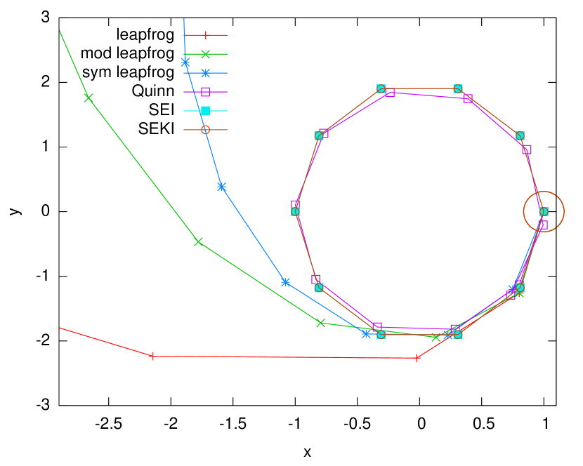
Figure 1: Particle motion during one epicycle using different integrators and a time-step $\Delta t=0.1\cdot 2\pi\Omega^{-1}$. The initial position, which is also the exact final position, is marked by a circle.

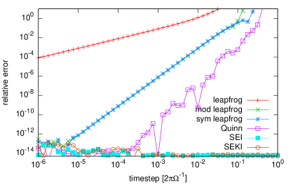
(a) Relative energy error as a function of time-step. Lower is better.

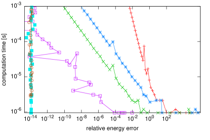
(b) Computation time as a function of relative energy error. Lower is better.

Figure 2: Epicyclic motion with no perturbing forces (Sect. 4.1). In this case SEI and SEKI follow the motion exactly. The method described in the Appendix was used to control round-off errors. The integration time is one epicycle period.

We first examine the case in which the perturbing force $\mathbf{f}$ in Eq. (1) vanishes, which corresponds to $m\rightarrow 0$ or $r_{\text{Hill}}\rightarrow 0$. In this case Hill’s equations of motion can be solved analytically and lead to epicyclic motion. We initialize the particle position to $\mathbf{r}=(1,0,0)^{T}$ and the velocity to $\mathbf{\dot{r}}=(0,-2,0)^{T}$, which corresponds to a trajectory that is a clockwise closed ellipse centered on the origin. We integrate the trajectory forward in time for one epicycle period ($t=2\pi\Omega^{-1}$).

To illustrate the behavior of each integrator, we use a relatively large time-step (one tenth of the epicycle period) and plot the position of the particle at every time-step in Figure 1. As expected, SEI and SEKI follow the analytic solution exactly. The Quinn et al. integrator yields an approximate ellipse but exhibits a phase error of $6^{\circ}$ per epicycle period. All three versions of the leapfrog integrator diverge badly from the analytic solution in less than one-quarter of an epicycle period.

In Figure 2a we plot the relative energy error as a function of the time-step. As expected, SEI and SEKI are exact to machine precision for all time-steps. The Quinn et al. integrator and the modified and symmetrized leapfrog integrators converge quadratically until machine precision is reached. Leapfrog converges only linearly. In Figure 2b we plot the computation time as a function of the relative error. This plot shows the fastest integrator for a desired precision. Of course, in this test case the choice is trivial, as SEI and SEKI give the exact solution for any time-step.

4.2 Perturbed epicyclic motion

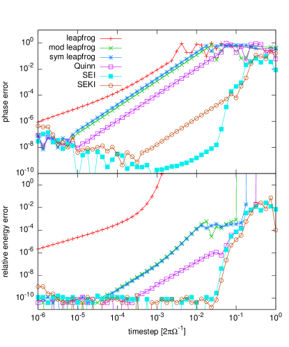
(a) Relative energy error and phase error as a function of time-step. Lower is better.

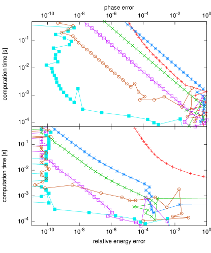
(b) Computation time as a function of relative energy error and phase error. Lower is better.

Figure 3: Perturbed epicyclic motion (Sect. 4.2). The trajectory passes the perturbing point mass at an impact parameter of $8\,r_{\text{Hill}}$. The integration time is 100 epicycle periods.

The motion of a test particle in the presence of a mass $m\neq 0$ can be described by a perturbed epicycle when the mass is sufficiently small, or, in other words, when the test particle is sufficiently far away from the mass or moving sufficiently fast, as quantified by Eq. (6). We place the particle initially on a circular orbit around mass $M$ (uniform motion along $\mathbf{e}_{y}$ in Hill’s approximation), with positions and velocities $\mathbf{r}=(5.55,2613.91,0)^{T}$ and $\mathbf{\dot{r}}=(0,-8.32,0)^{T}$. The trajectory passes the perturbing mass at an impact parameter corresponding to $8\,r_{\text{Hill}}$. The integration time is 100 epicycle periods. As an astrophysical example of such trajectories, we refer the reader to a study of the stochastic motion of moonlets embedded in Saturn’s rings by Rein & Papaloizou (2010).

In Figure 3 we plot the same diagnostics as in Figure 2 and additionally the phase error. We also looked at other measures of the accuracy of the integrators but do not show the results. SEI (for unbound orbits) and SEKI (for bound orbits, see below) perform at least as well as the other integrators tested by all measures that we have examined, and much better by most of them. SEI and SEKI also turn out to be exceptionally good at calculating the phase of the epicyclic motion.

One can see from Figure 3a that SEI and SEKI exhibit energy errors that are up to three orders of magnitude smaller than any other integrator for typical time-steps used in most simulations ($\Delta t\sim 10^{-3}$–$5\cdot 10^{-2})$. Eventually the errors are dominated by round-off errors ($\Delta t\lesssim 5\cdot 10^{-4}$) for all integrators. One can further see that at a fixed time-step SEI produces a phase error that is up to seven (!) orders of magnitude smaller than the error produced by the Quinn et al. integrator. From Figure 3b it is clear that SEI is also by far the fastest integrator for a given precision.

4.3 Strongly perturbed epicyclic motion

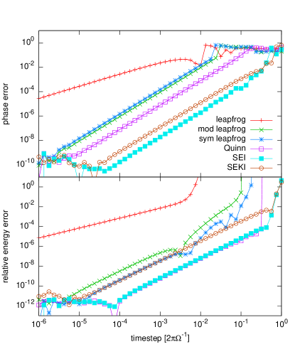
(a) Relative energy error and phase error as a function of time-step. Lower is better.

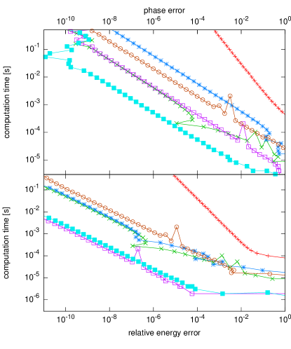
(b) Computation time as a function of relative energy error and phase error. Lower is better.

Figure 4: Strongly perturbed epicyclic motion (Sect. 4.3). The trajectory has an impact parameter of $1\,r_{\text{Hill}}$ corresponding to a horse-shoe orbit. The integration time is 100 epicycle periods.

We also performed tests in which we place the test particle on an orbit with an impact parameter of $1r_{\text{Hill}}$, so the perturbing forces are much stronger than in the previous case. The trajectory of the test particle is then a horse-shoe orbit.

In Figure 4 we plot the same diagnostics as in Figure 3 for this case. One can see that SEI and the Quinn et al. integrator perform equally well as measured by the energy error. However, the phase error is more than two orders of magnitude smaller using the SEI or the SEKI integrator rather than for any of the other integrators. Note that the SEKI integrator has significantly larger energy error than SEI. This is because for this test case all of the Hamiltonian operators in Eqs. (53) and (56) are roughly of the same magnitude and thus, the commutators of the operators that give rise to large integration errors. Because SEKI is based on a split into five operators while SEI is based on three, there are more commutators and the total error is larger in SEKI.

4.4 Perturbed Keplerian motion

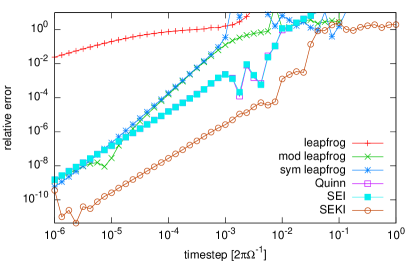
(a) Relative energy error as a function of time-step. Lower is better.

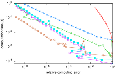
(b) Computation time as a function of relative error. Lower is better.

Figure 5: Perturbed Keplerian motion (Sect. 4.4). The initial orbit is circular with semi-major axis $0.18\,r_{\text{Hill}}$. The integration time is 10 epicycle periods or 226 orbital periods around the mass $m$.

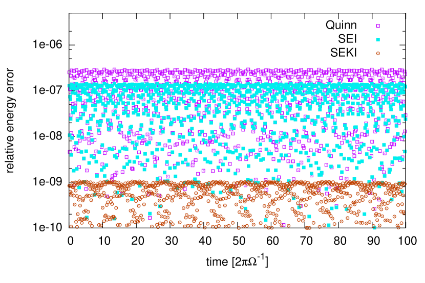
Figure 6: Relative energy error using different integrators and a time-step $\Delta t=10^{-5}\;2\pi\Omega^{-1}$. The algorithm described in Appendix A was used to minimize round-off errors.

We finally test the strong gravity regime, where the forces that govern the epicyclic motion can be viewed as a perturbation to a Keplerian orbit. The initial positions and velocities are $\mathbf{r}=(0.125,0,0)^{T}$ and $\mathbf{\dot{r}}=(0,-0.354,0)^{T}$, which correspond to an initially circular, bound orbit of $m_{1}$ and $m_{2}$. The semi-major axis of this orbit corresponds to $0.18r_{\text{Hill}}$. The integration time is ten epicycle periods, corresponding to 226 Kepler orbital periods.

In Figure 5 we plot again the same diagnostics as in Figure 2. The SEKI integrator is the most robust integrator in the sample, with the energy error at a given time-step more than two orders of magnitude smaller than its competitors. This performance comes with a drawback, as each time-step is computationally more expensive; nevertheless, at fixed energy error it is still more than one order of magnitude faster than its competitors. Its relative advantage improves further for orbits with smaller semi-major axis (relative to $r_{\text{Hill}}$).

Also note that for integrations in which the evaluation of forces is expensive (for example in a tree code), the SEKI integrator has a further advantage as it uses fewer time-steps.

Figure 6 shows the time evolution of the relative energy error in the integration with $\Delta t=10^{-5}\;2\pi\Omega^{-1}$. All integrators (except the various flavors of leapfrog which are far off the scale and therefore not plotted) show no sign of a linear drift in the energy error: the maximum error is independent of time. This good behavior is due to the symplectic nature of these integrators as well as the use of the procedure described in Appendix A to control round-off error. The SEKI integrator is more than two orders of magnitude better than any other integrator in this example.

5 Conclusions

We have presented two new integrators for studying the small-scale dynamics of disks using Hill’s approximation.

The first is a simple symplectic and time-reversible integrator for Hill’s equations of motion that we call symplectic epicycle integrator (SEI). In the absence of small-scale forces such as the self-gravitational forces of the disk particles, SEI solves Hill’s equations of motion (epicyclic motion) exactly; otherwise the error over a fixed time integral scales as $O(\epsilon\,\Delta t^{2})$ when the small-scale forces are $O(\epsilon)$. Numerical tests using a variety of measures have shown that SEI always converges much faster than various flavors of leapfrog, and often much faster than the Quinn et al. (2010) integrator. For small $\epsilon$ ($\epsilon\sim 3(r_{\text{Hill}}/r)^{3}\sim 0.01$) the phase error can be up to seven orders of magnitude smaller than the phase error from the Quinn et al. integrator at the same time-step (Figure 3a). The computational cost per time-step of SEI and the Quinn et al. integrator are equivalent. Although SEI is simple to code, a C implementation can be downloaded at http://sns.ias.edu/~rein/.

The second integrator is also symplectic and time-reversible and is called the symplectic epicycle-Kepler integrator (SEKI). This integrator is useful in following bound two-body orbits in the sheared sheet and in this case can yield errors that are several orders of magnitude smaller than SEI.

These integrators can be generalized in several ways. First, higher order integrators can be constructed by concatenating SEI and SEKI steps of varying lengths (e.g., Yoshida, 1993). Second, although the discussion in this paper has, for simplicity, focused on the three-body problem, SEI can be applied to the $N$-body problem using shear periodic boundary conditions (e.g., Richardson, 1994). The force $\mathbf{f}$ in Eq. (1) can also describe gas drag on particles, although in this case the dynamics is not described by a Hamiltonian so the advantage of a symplectic, time-reversible integrator is less clear.

The SEKI integrator can also be generalized beyond Hill’s approximation. For example, consider a test particle orbiting in the gravitational field of a binary star with masses $M_{1}$ and $M_{2}$. The Hamiltonian can be written as a sum of two Keplerian Hamiltonians minus the kinetic energy,

$$H\left(\mathbf{r},\mathbf{p}\right)=H_{\text{Kep,}M1}\left(\mathbf{r},\mathbf{p}\right)+H_{\text{Kep,}M2}\left(\mathbf{r},\mathbf{p}\right)-H_{\text{Kin}}\left(\mathbf{p}\right).$$ (58)

The first two terms can be solved exactly, and the last term is simply a drift. Thus, the analog of Eq. (56) provides a second-order accurate, symplectic and time-reversible integrator that is exact when the test-particle motion is dominated by the gravitational field from either body.

Appendix A Round-off error due to rotations

Floating-point operations on a computer are subject to rounding errors. The IEEE standard for floating-point arithmetic (IEEE 754) specifies the rounding algorithm and ensures that the rounding error for additions and multiplications is quasi-random. Thus, the rounding error should grow with time as $O(\varepsilon\cdot(t/\Delta t)^{1/2})$, where $\varepsilon$ is the machine precision.

Both the SEI and SEKI integrators use rotations, which are written in Eqs. (50) and (52) as a rotation matrix with angle $\phi=\Omega\Delta t$. However, operating with this matrix on a position vector $(x,y)$ will not in general preserve the norm $r=(x^{2}+y^{2})^{1/2}$ because numerically $\sin^{2}\phi+\cos^{2}\phi\neq 1$. Since $\phi$ is the same at every time-step, the error grows linearly with the number of operations, $O(\varepsilon\cdot t)$, much worse than the $O(\varepsilon\cdot t^{1/2})$ behavior described above (Petit, 1998, and references therein). This results in an undesirable linear drift in energy.

For other integrators that solve the Kepler problem using rotations, such as the Wisdom–Holman integrator, this problem is usually not important. This is because the rotation angle in the Kepler problem depends implicitly on radius (Kepler’s law) and thus the rotation is actually a so-called twist map. There exists a KAM-like theorem (Blank et al., 1997) for twist maps that restricts the solution to an invariant torus in phase space.

Petit (1998) describes one way to solve this problem by decomposing the rotation operator in Eq. (50) into three shear operators

$$\left(\begin{array}[]{cc}\cos\phi&\sin\phi\\ -\sin\phi&\cos\phi\end{array}\right)=$$ (61)

$$\quad\quad\left(\begin{array}[]{cc}1&0\\ -\tan\tfrac{1}{2}\phi&1\end{array}\right)\cdot\left(\begin{array}[]{cc}1&\sin\phi\\ 0&1\end{array}\right)\cdot\left(\begin{array}[]{cc}1&0\\ -\tan\tfrac{1}{2}\phi&1\end{array}\right).$$ (68)

Why does this help? Suppose we replace the rotation matrix in Eq. (50) by an arbitrary matrix $\bf R$. It is then straightforward to show that the transformation from $(x^{n},y^{n},p_{x}^{n},p_{y}^{n})^{T}$ to $(x^{n+1},y^{n+1},p_{x}^{n+1},p_{y}^{n+1})^{T}$ defined by Eqs. (48) to (51) is symplectic if and only if $\mbox{det}\,{\bf R}=1$. Since 1 and 0 are represented exactly in floating-point arithmetic, each of the matrices on the right side of Eq. (68) has a determinant of exactly 1. Thus the transformation is symplectic whether or not $\sin\phi$ and $\tan{\textstyle{\frac{1}{2}}}\phi$ are related by the appropriate trigonometric identity, and hence is insensitive to round-off errors in evaluating these functions.

We tested both implementations of the rotation operator, Eq. (50) and Eq. (68). As expected, the implementation using shear operators shows no sign of a linear drift in energy (Figure 6). In contrast, for the test case presented in Figure 6, the straightforward implementation of Eq. (50) produces a linear drift of about $10^{-7}$ after only 100 epicycle periods. The additional computational cost of implementing the rotations using shear operators is negligible, and in long integrations this refinement can dramatically improve the accuracy.

References

- Bai & Stone (2010) Bai X., Stone J. M., 2010, ApJS, 190, 297
- Binney & Tremaine (2008) Binney J., Tremaine S., 2008, Galactic Dynamics: Second Edition. Princeton University Press
- Blank et al. (1997) Blank M., Kruger T., Pustyl’nikov L., 1997, ArXiv e-prints
- Crida et al. (2010) Crida A., Papaloizou J. C. B., Rein H., Charnoz S., Salmon J., 2010, AJ, 140, 944
- Goldreich & Lynden-Bell (1965) Goldreich P., Lynden-Bell D., 1965, MNRAS, 130, 125
- Goldreich & Tremaine (1978) Goldreich P., Tremaine S., 1978, ApJ, 222, 850
- Hawley & Balbus (1992) Hawley J. F., Balbus S. A., 1992, ApJ, 400, 595
- Heggie (2001) Heggie D. C., 2001, in B. A. Steves & A. J. Maciejewski ed., The Restless Universe . pp 109–128
- Hénon & Petit (1986) Hénon M., Petit J., 1986, Cel. Mech., 38, 67
- Hill (1878) Hill G. W., 1878, Astr. Nach., 91, 251
- Johansen et al. (2009) Johansen A., Youdin A., Mac Low M., 2009, ApJ, 704, L75
- Julian & Toomre (1966) Julian W. H., Toomre A., 1966, ApJ, 146, 810
- Kinoshita et al. (1991) Kinoshita H., Yoshida H., Nakai H., 1991, Cel. Mech. Dyn. Astr., 50, 59
- Mikkola & Merritt (2006) Mikkola S., Merritt D., 2006, MNRAS, 372, 219
- Petit (1998) Petit J., 1998, Celestial Mechanics and Dynamical Astronomy, 70, 1
- Quinn et al. (2010) Quinn T., Perrine R. P., Richardson D. C., Barnes R., 2010, AJ, 139, 803
- Rein et al. (2010) Rein H., Lesur G., Leinhardt Z. M., 2010, A&A, 511, A69
- Rein & Papaloizou (2010) Rein H., Papaloizou J. C. B., 2010, A&A, 524, A22
- Richardson (1994) Richardson D. C., 1994, MNRAS, 269, 493
- Saha & Tremaine (1992) Saha P., Tremaine S., 1992, AJ, 104, 1633
- Salo (1992) Salo H., 1992, Nature, 359, 619
- Springel (2005) Springel V., 2005, MNRAS, 364, 1105
- Stone & Gardiner (2010) Stone J. M., Gardiner T. A., 2010, ApJS, 189, 142
- Tanga et al. (2004) Tanga P., Weidenschilling S. J., Michel P., Richardson D. C., 2004, A&A, 427, 1105
- Wadsley et al. (2004) Wadsley J. W., Stadel J., Quinn T., 2004, New Astronomy, 9, 137
- Wisdom & Holman (1991) Wisdom J., Holman M., 1991, AJ, 102, 1528
- Wisdom & Tremaine (1988) Wisdom J., Tremaine S., 1988, AJ, 95, 925
- Yoshida (1993) Yoshida H., 1993, Cel. Mech. Dyn. Astr., 56, 27