Design of Strict Control-Lyapunov Functions
for Quantum Systems with QND Measurements

Abstract

We consider discrete-time quantum systems subject to Quantum Non-Demolition (QND) measurements and controlled by an adjustable unitary evolution between two successive QND measures. In open-loop, such QND measurements provide a non-deterministic preparation tool exploiting the back-action of the measurement on the quantum state. We propose here a systematic method based on elementary graph theory and inversion of Laplacian matrices to construct strict control-Lyapunov functions. This yields an appropriate feedback law that stabilizes globally the system towards a chosen target state among the open-loop stable ones, and that makes in closed-loop this preparation deterministic. We illustrate such feedback laws through simulations corresponding to an experimental setup with QND photon counting.

1 Introduction

Feedback stabilization of quantum states is closely related to the concept of Quantum Non-Demolition (QND) measurement [3, 12, 13]. Indeed, as soon as we are interested in applying a measurement-based feedback to stabilize a quantum state, we need to make sure that the measurement itself is not changing the desired target state. This means that the measurement procedure is QND with respect to the projection over the target state. In fact, very often a well-chosen QND measurement protocol can itself be considered as a preparation tool for various quantum states. However, this preparation is generally non-deterministic and one can not make sure to converge towards the desired state except by repeating the experiment many times. The feedback can be applied here to make this process deterministic [11, 8, 4].

This paper is a generalization of the feedback law, proposed in [4, 7] and experimentally tested in [9], to generic discrete-time quantum systems where, between two successive QND measurements, a controlled unitary evolution can be applied. The dynamics of such discrete-time quantum systems are governed by non linear Markov chains. In [4, 7] the feedback laws were obtained by maximizing the fidelity with respect to the target state at each time-step: this means that the feedback strategy was based on the same Lyapunov function given by the fidelity between the current and the target state. We propose here a systematic and explicit method to design a new family of control-Lyapunov functions. The main interest of these new Lyapunov functions relies on the crucial fact that the increases of their expectation values at step $k+1$ knowing the state $\rho_{k}$ at step $k$ remain strictly positive when $\rho_{k}$ does not coincide with the target state. In closed-loop, these Lyapunov functions become strict and the convergence analysis is notably simplified since invariance principles are not necessary. The construction of these strict Lyapunov functions is based on the Hamiltonian $H$ underlying the controlled unitary evolution and relies on the connectivity of the graph attached to $H$. They are obtained by inverting a Laplacian matrix derived from $H$ and the quantum states that are untouched by the QND measurements.

In section 2, we describe the finite dimensional Markovian model together with the main modeling assumptions. Section 3 is devoted to the open-loop behavior (Theorem 3.1) that can be seen as a non-deterministic protocol for preparing a finite number of isolated and orthogonal quantum states. In Section 4, we present the main ideas underlying the construction of these strict control-Lyapunov functions $W_{\epsilon}$. Then we define the connectivity graph, the Laplacian matrix attached to $H$ and two technical lemmas used during this construction. Finally Theorem 4.1 describes the stabilizing feedback derived from $W_{\epsilon}$. Closed-loop simulations corresponding to an experimental setup at Ecole Normale Supérieure are sketched in section 5.

The authors thank M. Brune, I. Dotsenko, S. Gleyzes, S. Haroche and J.M. Raimond for enlightening discussions and references. Advices of L. Praly concerning control-Lyapunov functions are also acknowledged.

2 The non-linear Markov model

We consider a finite dimensional quantum system (the underlying Hilbert space ${\mathcal{H}}={\mathbb{C}}^{d}$ is of dimension $d>0$) being measured through a generalized measurement procedure placed discretely in time. Between two measurements, the system undergoes a unitary evolution depending on a scalar control input $u\in{\mathbb{R}}$. The dynamics of such discrete time quantum systems is described by a non-linear controlled Markov chain whose structure is derived from quantum physics. We just sketch here this structure with a mathematical viewpoint. A tutorial physical exposure can be found in [5].

The system state is described by the density operator $\rho$ belonging to ${\mathcal{D}}({\mathcal{H}})$ the set of positive, Hermitian matrices of trace one:

$${\mathcal{D}}({\mathcal{H}}):=\{\rho\in{\mathbb{C}}^{d\times d}\leavevmode\nobreak\ |\quad\rho=\rho^{\dagger},\quad\text{Tr}\left(\rho\right)=1,\quad\rho\geq 0\}.$$

The generalized measurement procedure admits $m>0$ different discrete values $\mu\in\{1,\ldots,m\}$: to each measurement outcome $\mu$ is attached a Kraus operator described by a matrix $M_{\mu}\in{\mathbb{C}}^{d\times d}$. The Kraus operators $(M_{\mu})_{\mu\in\{1,\ldots,m\}}$ satisfy the constraint $\sum_{\mu=1}^{m}M_{\mu}^{{\dagger}}M_{\mu}={{1\!\!1}}$ where ${{1\!\!1}}$ is the identity matrix. In general the $M_{\mu}$ are not necessarily Hermitian. The controlled evolution between two measures $U_{u}$ is defined by the unitary operator $\exp(-iuH)=U_{u}$ where $H$ is a Hermitian operator $H\in{\mathbb{C}}^{d\times d}$ with $H^{\dagger}=H$.

The random evolution of the state $\rho_{k}\in{\mathcal{D}}({\mathcal{H}})$ at time step $k$ is modeled through the following Markov process:

$$\rho_{k+1}={\mathbb{U}}_{u_{k}}({\mathbb{M}}_{\mu_{k}}(\rho_{k})),$$ (1)

where

• $u_{k}\in{\mathbb{R}}$ is the control at step $k$,

• $\mu_{k}$ is a random variable taking values $\mu$ in $\{1,\cdots,m\}$ with probability $p_{\mu,\rho_{k}}=\text{Tr}\left(M_{\mu}\rho_{k}M_{\mu}^{\dagger}\right)$,

• ${\mathbb{U}}_{u}$ is the super-operator

  $${\mathbb{U}}_{u}:\quad{\mathcal{D}}({\mathcal{H}})\ni\rho\mapsto U_{u}\rho U_{u}^{\dagger}\in{\mathcal{D}}({\mathcal{H}}),$$

• For each $\mu$, ${\mathbb{M}}_{\mu}$ is the super-operator

  $${\mathbb{M}}_{\mu}:\quad\rho\mapsto\tfrac{M_{\mu}\rho M_{\mu}^{\dagger}}{\text{Tr}\left(M_{\mu}\rho M_{\mu}^{{\dagger}}\right)}\in{\mathcal{D}}({\mathcal{H}})$$

  defined for $\rho\in{\mathcal{D}}({\mathcal{H}})$ such that $\text{Tr}\left(M_{\mu}\rho M_{\mu}^{\dagger}\right)\neq 0$.

We suppose throughout this paper that the two following assumptions are verified by the system under consideration.

Assumption 1.

The measurement operators $M_{\mu}$ are diagonal in the same orthonormal basis $\{\,\left|n\right>\,|\quad n\in\{1,\cdots,d\}\}$, therefore $M_{\mu}=\sum_{n=1}^{d}c_{\mu,n}\left|n\right>\left<n\right|$ with $c_{\mu,n}\in{\mathbb{C}}.$

Assumption 2.

For all $n_{1}\neq n_{2}$ in $\{1,\cdots,d\},$ there exists a $\mu\in\{1,\cdots,m\}$ such that $|c_{\mu,n_{1}}|^{2}\neq|c_{\mu,n_{2}}|^{2}.$

Assumption 1 means that the considered measurement process achieves a Quantum Non Demolition (QND) measurement for the physical observables given by orthogonal projections over the states $\bigl{\{}\left|n\right>\,|\quad n\in\{1,\cdots,d\}\bigr{\}}.$ This implies that for $u_{k}\equiv 0$, any $\rho=\left|n\right>\left<n\right|$ corresponding to the orthogonal projector on the basis vector $\left|n\right>$, $n\in\{1,\ldots,d\}$, is a fixed point of the Markov process (1). Since the operators $M_{\mu}$ must satisfy $\sum_{\mu=1}^{m}M_{\mu}^{{\dagger}}M_{\mu}={{1\!\!1}}$, we have, according to assumption 1, $\sum_{\mu=1}^{m}|c_{\mu,n}|^{2}=1$ for all $n\in\{1,\cdots,d\}.$

Assumption 2 means that there exists a $\mu$ such that the statistics when $u_{k}\equiv 0$ for obtaining the measurement result $\mu$ are different for the fixed points $\left|n_{1}\right>\left<n_{1}\right|$ and $\left|n_{2}\right>\left<n_{2}\right|$. This follows by noting that $\text{Tr}\left(M_{\mu}\left|n\right>\left<n\right|M_{\mu}^{\dagger}\right)=|c_{\mu,n}|^{2}$ for $n\in\{1,\cdots,d\}$.

3 Convergence of the open-loop dynamics

When the control vanishes ($u_{k}=0,\leavevmode\nobreak\ \forall k$), the dynamics is simply given by

$$\rho_{k+1}={\mathbb{M}}_{\mu_{k}}(\rho_{k})$$ (2)

where $\mu_{k}$ is a random variable with discrete values in $\{1,\ldots,m\}$. The probability $p_{\mu,\rho_{k}}$ to have $\mu_{k}=\mu$ depends on $\rho_{k}$: $p_{\mu,\rho_{k}}=\text{Tr}\left(M_{\mu}\rho_{k}M_{\mu}^{\dagger}\right)$. We have then the following theorem characterizing the open-loop asymptotic behavior:

Theorem 3.1.

Consider a Markov process $\rho_{k}$ obeying the dynamics of (2) with an initial condition $\rho_{0}$ in ${\mathcal{D}}({\mathcal{H}})$. Then

• with probability one, $\rho_{k}$ converges to one of the $d$ states $\left|n\right>\left<n\right|$ with $n\in\{1,\cdots,d\}.$

• the probability of convergence towards the state $\left|n\right>\left<n\right|$ depends only on the initial condition $\rho_{0}$ and is given by

  $$\text{Tr}\left(\rho_{0}\left|n\right>\left<n\right|\right)=\left<n\right|\rho_{0}\left|n\right>.$$

The proof is a generalization of the one given in [1].

Proof.

For any $n\in\{1,\ldots,d\}$, $\text{Tr}\left(\left|n\right>\left<n\right|\rho\right)$ is a martingale. This results from

$${\text{\normalsize$\mathbb{E}$}}\left(\text{Tr}\left(\left|n\right>\left<n\right|\rho_{k+1}\right)|\rho_{k}\right)\\ =\sum_{\mu=1}^{m}\text{Tr}\left(M_{\mu}\rho_{k}M_{\mu}^{\dagger}\right)\text{Tr}\left(\left|n\right>\left<n\right|{\mathbb{M}}_{\mu}(\rho_{k})\right)\\ =\sum_{\mu=1}^{m}\text{Tr}\left(\left|n\right>\left<n\right|M_{\mu}\rho_{k}M_{\mu}^{\dagger}\right)=\text{Tr}\left(\sum_{\mu=1}^{m}M_{\mu}^{{\dagger}}M_{\mu}\left|n\right>\left<n\right|\rho_{k}\right)\\ =\text{Tr}\left(\left|n\right>\left<n\right|\rho_{k}\right),$$

where we have used the facts that $M_{\mu}$ and $\left|n\right>\left<n\right|$ commute and that $\sum_{\mu=1}^{m}M_{\mu}^{\dagger}M_{\mu}={1\!\!1}$. Take the function

$$V(\rho):=\sum_{n=1}^{d}f(\text{Tr}\left(\left|n\right>\left<n\right|\rho\right)).$$ (3)

where $f(x)=\tfrac{x^{2}}{2}$. The function $f$ being convex and each $\text{Tr}\left(\left|n\right>\left<n\right|\rho\right)$ being a martingale, we infer that $V(\rho)$ is a sub-martingale

$${\text{\normalsize$\mathbb{E}$}}\left(V(\rho_{k+1})|\rho_{k}\right)\geq V(\rho_{k}).$$

More precisely, we have

$${\text{\normalsize$\mathbb{E}$}}\left(V(\rho_{k+1})|\rho_{k}\right)=\\ \sum_{n=1}^{d}\sum_{\mu\in I_{\rho_{k}}}\text{Tr}\left(M_{\mu}\rho_{k}M_{\mu}^{\dagger}\right)f\left(\tfrac{\text{Tr}\left(\left|n\right>\left<n\right|M_{\mu}\rho_{k}M_{\mu}^{\dagger}\right)}{\text{Tr}\left(M_{\mu}\rho_{k}M_{\mu}^{\dagger}\right)}\right),$$

with $I_{\rho_{k}}=\Bigl{\{}\mu\in\{1,\cdots,m\}\leavevmode\nobreak\ |\leavevmode\nobreak\ \text{Tr}\left(M_{\mu}\rho_{k}M_{\mu}^{\dagger}\right)\neq 0\Bigr{\}}$. For all sequence of reals $x_{1},\cdots,x_{m}$ and $\theta_{1},\cdots,\theta_{m}$ in the interval $[0,1]$ with $\sum_{\mu=1}^{m}\theta_{\mu}=1$, we have the identity

$$\sum_{\mu=1}^{m}\theta_{\mu}f(x_{\mu})=f\left(\sum_{\mu=1}^{m}\theta_{\mu}x_{\mu}\right)+\sum_{\mu,\nu=1}^{m}\theta_{\mu}\theta_{\nu}\tfrac{(x_{\mu}-x_{\nu})^{2}}{4}.$$ (4)

For each $\mu$, let $\theta_{\mu}=\text{Tr}\left(M_{\mu}\rho_{k}M_{\mu}^{\dagger}\right)$, $x_{\mu}=\tfrac{\text{Tr}\left(\left|n\right>\left<n\right|M_{\mu}\rho_{k}M_{\mu}^{\dagger}\right)}{\text{Tr}\left(M_{\mu}\rho_{k}M_{\mu}^{\dagger}\right)}$ if $\theta_{\mu}>0$ and $x_{\mu}=0$ otherwise. Identity (4) yields

$${\text{\normalsize$\mathbb{E}$}}\left(V(\rho_{k+1})|\rho_{k}\right)-V(\rho_{k})=\\ \tfrac{1}{4}\sum_{n=1}^{d}\sum_{\mu,\nu\in I_{\rho_{k}}}\text{Tr}\left(M_{\mu}\rho_{k}M_{\mu}^{\dagger}\right)\text{Tr}\left(M_{\nu}\rho_{k}M_{\nu}^{\dagger}\right)\ldots\\ \ldots\left(\tfrac{|c_{\mu,n}|^{2}\left<n\right|\rho_{k}\left|n\right>}{\text{Tr}\left(M_{\mu}\rho_{k}M_{\mu}^{\dagger}\right)}-\tfrac{|c_{\nu,n}|^{2}\left<n\right|\rho_{k}\left|n\right>}{\text{Tr}\left(M_{\nu}\rho_{k}M_{\nu}^{\dagger}\right)}\right)^{2}.$$ (5)

We have used the fact that $\left<n\right|{\mathbb{M}}_{\mu}(\rho_{k})\left|n\right>=\frac{|c_{\mu,n}|^{2}\left<n\right|\rho_{k}\left|n\right>}{\text{Tr}\left(M_{\mu}\rho_{k}M_{\mu}^{\dagger}\right)}$. Thus, $V(\rho_{k})$ is a sub-martingale, and in addition we have a precise bound on the difference ${\text{\normalsize$\mathbb{E}$}}\left(V(\rho_{k+1})|\rho_{k}\right)-V(\rho_{k})$. We denote by $Q(\rho_{k})$ the right term in Equation (5). Note that the sum in the definition of $Q(\rho_{k})$ is over all $\mu,\nu\in I_{\rho_{k}}$. However, we can assume that the sum is actually over all $\mu,\nu$ in $\{1,\cdots,m\}$ by observing the following facts.

For any $\mu,\nu$, take the mapping

$$\rho\mapsto\text{Tr}\left(M_{\mu}\rho M_{\mu}^{\dagger}\right)\text{Tr}\left(M_{\nu}\rho M_{\nu}^{\dagger}\right)\left(\tfrac{|c_{\mu,n}|^{2}\left<n\right|\rho\left|n\right>}{\text{Tr}\left(M_{\mu}\rho M_{\mu}^{\dagger}\right)}-\tfrac{|c_{\nu,n}|^{2}\left<n\right|\rho\left|n\right>}{\text{Tr}\left(M_{\nu}\rho M_{\nu}^{\dagger}\right)}\right)^{2}$$

defined only when $\text{Tr}\left(M_{\mu}\rho M_{\mu}^{\dagger}\right)\text{Tr}\left(M_{\nu}\rho M_{\nu}^{\dagger}\right)>0$. Since this mapping is positive and bounded by $\rho\mapsto\text{Tr}\left(M_{\mu}\rho M_{\mu}^{\dagger}\right)\text{Tr}\left(M_{\nu}\rho M_{\nu}^{\dagger}\right)$, it can be extended by continuity to any $\rho\in{\mathcal{D}}({\mathcal{H}})$ by taking a null value when $\text{Tr}\left(M_{\mu}\rho M_{\mu}^{\dagger}\right)\text{Tr}\left(M_{\nu}\rho M_{\nu}^{\dagger}\right)=0$. Thus

$$Q(\rho)=\tfrac{1}{4}\sum_{n=1}^{d}\sum_{\mu,\nu=1}^{m}\text{Tr}\left(M_{\mu}\rho M_{\mu}^{\dagger}\right)\text{Tr}\left(M_{\nu}\rho M_{\nu}^{\dagger}\right)\\ \left(\tfrac{|c_{\mu,n}|^{2}\left<n\right|\rho\left|n\right>}{\text{Tr}\left(M_{\mu}\rho M_{\mu}^{\dagger}\right)}-\tfrac{|c_{\nu,n}|^{2}\left<n\right|\rho\left|n\right>}{\text{Tr}\left(M_{\nu}\rho M_{\nu}^{\dagger}\right)}\right)^{2}$$ (6)

is continuously defined for any $\rho\in{\mathcal{D}}({\mathcal{H}})$ and still satisfies

$${\text{\normalsize$\mathbb{E}$}}\left(V(\rho_{k+1})|\rho_{k}\right)-V(\rho_{k})=Q(\rho_{k}),\forall\rho_{k}\in{\mathcal{D}}({\mathcal{H}}).$$

By Theorem A.1 of the Appendix, the $\omega$-limit set $\Omega$ (in the sense of almost sure convergence), for the trajectories $\rho_{k}$, is a subset of the set $\{\rho\in{\mathcal{D}}({\mathcal{H}})|\quad Q(\rho)=0\}.$

Let us consider a density matrix $\rho_{\infty}$ in the $\omega$-limit set. Therefore $Q(\rho_{\infty})=0$ implies

$$\tfrac{|c_{\mu,n}|^{2}\left<n\right|\rho_{\infty}\left|n\right>}{\text{Tr}\left(M_{\mu}\rho_{\infty}M_{\mu}^{\dagger}\right)}-\tfrac{|c_{\nu,n}|^{2}\left<n\right|\rho_{\infty}\left|n\right>}{\text{Tr}\left(M_{\nu}\rho_{\infty}M_{\nu}^{\dagger}\right)}\,=0,$$ (7)

for all $\mu$ and $\nu$ in $I_{\rho_{\infty}}$ and for each basis element $\left|n\right>$. Since $\text{Tr}\left(\rho_{\infty}\right)=1,$ there is at least one $\bar{n}$ such that $\left<\bar{n}\right|\rho_{\infty}\left|\bar{n}\right>>0$. Then Equation (7) simplifies to

$$\text{Tr}\left(M_{\mu}\rho_{\infty}M_{\mu}^{\dagger}\right)|c_{\nu,\bar{n}}|^{2}=\text{Tr}\left(M_{\nu}\rho_{\infty}M_{\nu}^{\dagger}\right)|c_{\mu,\bar{n}}|^{2},$$

for all $\mu,\nu\in I_{\rho_{\infty}}$. Summing over $\nu\in I_{\rho_{\infty}}$, we find

$$\text{Tr}\left(M_{\mu}\rho_{\infty}M_{\mu}^{\dagger}\right)\,\Bigl{(}\sum_{\nu\in I_{\rho_{\infty}}}|c_{\nu,\bar{n}}|^{2}\Bigr{)}=\\ \Bigl{(}\sum_{\nu\in I_{\rho_{\infty}}}\text{Tr}\left(M_{\nu}\rho_{\infty}M_{\nu}^{\dagger}\right)\Bigr{)}\,|c_{\mu,\bar{n}}|^{2}$$

By definition of $I_{\rho_{\infty}}$

$$\sum_{\nu\in I_{\rho_{\infty}}}\text{Tr}\left(M_{\nu}\rho_{\infty}M_{\nu}^{\dagger}\right)=\sum_{\nu=1}^{m}\text{Tr}\left(M_{\nu}\rho_{\infty}M_{\nu}^{\dagger}\right)=1.$$

Thus we have

$$\text{Tr}\left(M_{\mu}\rho_{\infty}M_{\mu}^{\dagger}\right)\Bigl{(}\sum_{\nu\in I_{\rho_{\infty}}}|c_{\nu,\bar{n}}|^{2}\Bigr{)}=|c_{\mu,\bar{n}}|^{2}.$$

For $\nu\notin I_{\rho_{\infty}}$, $c_{\nu,\bar{n}}=0$ since $\sum_{n=1}^{d}|c_{\nu,n}|^{2}\left<n\right|\rho_{\infty}\left|n\right>=0$, each $\left<n\right|\rho_{\infty}\left|n\right>\geq 0$ and $\left<\bar{n}\right|\rho_{\infty}\left|\bar{n}\right>>0$. Thus $\sum_{\nu\in I_{\rho_{\infty}}}|c_{\nu,\bar{n}}|^{2}=\sum_{\nu=1}^{m}|c_{\nu,\bar{n}}|^{2}=1$. Finally, we have

$$\forall\mu\in I_{\rho_{\infty}},\quad\text{Tr}\left(M_{\mu}\rho_{\infty}M_{\mu}^{\dagger}\right)=|c_{\mu,\bar{n}}|^{2}.$$ (8)

as soon as $\left<\bar{n}\right|\rho_{\infty}\left|\bar{n}\right>>0$.

Assume now that exist $\bar{n}_{1}\neq\bar{n}_{2}$ in $\{1,\ldots,d\}$ such that $\left<\bar{n}_{1}\right|\rho_{\infty}\left|\bar{n}_{1}\right>>0$ and $\left<\bar{n}_{2}\right|\rho_{\infty}\left|\bar{n}_{2}\right>>0$. Then (8) implies that

$$\forall\mu\in I_{\rho_{\infty}},\quad|c_{\mu,\bar{n}_{1}}|^{2}=|c_{\mu,\bar{n}_{2}}|^{2}.$$ (9)

By Assumption 2, there exists a $\bar{\mu}\in\{1,\cdots,m\}$ such that $|c_{\bar{\mu},\bar{n}_{1}}|^{2}\neq|c_{\bar{\mu},\bar{n}_{2}}|^{2}$. These terms cannot be simultaneously zero, thus $\text{Tr}\left(M_{\bar{\mu}}\rho_{\infty}M_{\bar{\mu}}^{\dagger}\right)>0$, $\bar{\mu}\in I_{\rho_{\infty}}$. This is in contradiction with (9). This closes the proof of the assertion: the $\omega$-limit set is reduced to the set fixed point $\left|n\right>\left<n\right|,$ with $n\in\{1,\cdots,d\}$.

We have shown that the probability measure associated to the random variable $\rho_{k}$ converges to the probability measure $\sum_{n=1}^{d}p_{n}\delta_{\left|n\right>\left<n\right|},$ where $\delta_{\left|n\right>\left<n\right|}$ denotes the Dirac measure at $\left|n\right>\left<n\right|$ and $p_{n}$ is the probability of convergence towards $\left|n\right>\left<n\right|.$ In particular, we have ${\text{\normalsize$\mathbb{E}$}}\left(\text{Tr}\left(\rho_{k}\left|n\right>\left<n\right|\right)\right)\longrightarrow p_{n}.$ But $\text{Tr}\left(\left|n\right>\left<n\right|\rho_{k}\right)$ is a martingale thus ${\text{\normalsize$\mathbb{E}$}}\left(\text{Tr}\left(\left|n\right>\left<n\right|\rho_{k}\right)\right)={\text{\normalsize$\mathbb{E}$}}\left(\text{Tr}\left(\left|n\right>\left<n\right|\rho_{0}\right)\right)$ and consequently $p_{n}=\left<n\right|\rho_{0}\left|n\right>$. ∎

4 Feedback stabilization

4.1 Design of strict control-Lyapunov functions

The goal is to design a feedback law that globally stabilizes the Markov chain (1) towards a chosen target state $\left|\bar{n}\right>\left<\bar{n}\right|$, for some $\bar{n}$ among $\{1,\cdots,d\}$. In previous publications [8, 7, 4], the proposed feedback schemes tend to increase at each step the same open-loop martingale $V_{\bar{n}}(\rho)=\left<\bar{n}\right|\rho\left|\bar{n}\right>$: $u$ is chosen in order to increase $u\mapsto V_{\bar{n}}({\mathbb{U}}_{u}(\rho))$. When $\rho=\left|n\right>\left<n\right|$ with $n\neq\bar{n}$, $u\mapsto V_{n}(\rho)$ is minimum at $u=0$. Consequently, its first-order $u$-derivative vanishes at $u=0$. But its second-order $u$-derivative could also vanishe at $u=0$. For the photon-box considered in [4] (see also section 5), this happens when $|n-\bar{n}|\geq 2$. Such lack of strong convexity in $u$ when the image of $\rho$ is almost orthogonal to $\left|\bar{n}\right>$, explains the fact that, in previous works, the control $u$ is set to a constant non-zero value when $V_{\bar{n}}(\rho)$ is close to $0$,

To improve convergence and avoid such constant feedback zone, we propose to modify $V_{\bar{n}}$ using the other open-loop martingales $V_{n}(\rho)=\left<n\right|\rho\left|n\right>$ and the sub-martingale $V(\rho)=\sum_{n=1}^{d}(\left<n\right|\rho\left|n\right>)^{2}$ used during the proof of theorem 3.1. The goal of such modification is to get control Lyapunov functions still admitting a unique global maximum at $\left|\bar{n}\right>\left<\bar{n}\right|$ but being strongly convex versus $u$ around $0$ when $\rho$ is close to any $\left|n\right>\left<n\right|$, $n\neq\bar{n}$.

Take $W_{0}(\rho)=\sum_{n=1}^{d}\sigma_{n}\left<n\right|\rho\left|n\right>$ with real coefficients $\sigma_{n}$ to be chosen such that $\sigma_{\bar{n}}$ remains the largest one and such that, for any $n\neq\bar{n}$, the second-order $u$-derivative of $W_{0}({\mathbb{U}}_{u}(\left|n\right>\left<n\right|))$ at $u=0$ is strictly positive. This yields to a set of linear equations (see lemma 4.2) in $\sigma_{n}$ that can be solved by inverting a Laplacian matrix (see lemma 4.1). Notice that $W_{0}$ is an open-loop martingale. To obtain a sub-martingale we consider (see theorem 4.1) $W_{\epsilon}(\rho)=W_{0}(\rho)+\epsilon V(\rho)$. For $\epsilon>0$ small enough: $W_{\epsilon}(\rho)$ still admits a unique global maximum at $\left|\bar{n}\right>\left<\bar{n}\right|$; for $u$ close to $0$, $W_{\epsilon}({\mathbb{U}}_{u}(\left|n\right>\left<n\right|))$ is strongly convex for any $n\neq\bar{n}$ and strongly concave for $n=\bar{n}$. This implies that $W_{\epsilon}$ is a control-Lyapunov function with arbitrary small control (see proof of theorem 4.1).

Let us continue by some definitions and lemmas that underlay the construction of these strict control-Lyapunov functions $W_{\epsilon}$.

4.2 Connectivity graph and Laplacian matrix

To the Hamiltonian operator $H$ defining the controlled unitary evolution $U_{u}=e^{-\imath uH}$, we associate its undirected connectivity graph denote by $G^{H}$. This graph admits $d$ vertices labeled by $n\in\{1,\ldots,d\}$. Two different vertices $n_{1}\neq n_{2}$ ($n_{1},n_{2}\in\{1,\ldots,d\}$) are linked by an edge, if and only if, $\left<n_{1}\right|H\left|n_{2}\right>\neq 0$. Attached to $H$, we also associate $R^{H}$, the real symmetric matrix $d\times d$ (Laplacian matrix) with entries

$$R^{H}_{n_{1},n_{2}}=2\Big{(}\delta_{n_{1},n_{2}}\left<n_{1}\right|H^{2}\left|n_{2}\right>-|\left<n_{1}\right|H\left|n_{2}\right>|^{2}\Big{)}.$$ (10)

Lemma 4.1.

Assume the graph $G^{H}$ to be connected. Then for any positive reals $\lambda_{n}$, $n\in\{1,\ldots,d\}$, $n\neq\bar{n}$, there exists a vector $\sigma=(\sigma_{n})_{n\in\{1,\ldots,d\}}$ of ${\mathbb{R}}^{d}$ such that $R^{H}\sigma=-\lambda$ where $\lambda$ is the vector of ${\mathbb{R}}^{d}$ of components $\lambda_{n}$ for $n\neq\bar{n}$ and $\lambda_{\bar{n}}=-\sum_{n\neq\bar{n}}\lambda_{n}$.

Proof.

Note that $R^{H}$ is symmetric and the sum of the entries for any column and any row of $R^{H}$ is equal to zero. Therefore, the vector $(1\cdots 1)^{T}$ is in the kernel of $R^{H}$. The diagonal (resp.non-diagonal) components of $R^{H}$ are positive (resp. negative). Therefore $R^{H}$ is a Laplacian matrix (see [2, Ch. 4]). The connectivity graph associated to $R^{H}$ coincides with $G^{H}$. Since this graph is supposed connected, classical results of graph theory (see, e.g., [2, Theorem $3.1$]) imply that the ”constant” vector $(1,\cdots,1)^{T}$ spans the kernel of $R^{H}$. Therefore, the dimension of the image of $R^{H}$ is equal to $d-1$. Since $R^{H}$ is symmetric, its image coincides with the orthogonal to its kernel. For the sake of completeness, here we give a simple proof of this statement. Indeed, for any vector $X$ in the kernel of $R^{H}$, we have

$$\sum_{n_{1},n_{2}\in\{1,\cdots,d\}}R^{H}_{n_{1},n_{2}}(X_{n_{1}}-X_{n_{2}})^{2}=X^{T}RX=0.$$

This implies $R^{H}_{n_{1},n_{2}}(X_{n_{1}}-X_{n_{2}})^{2}=0$, $\forall n_{1},n_{2}\in\{1,\cdots,d\}$. As the graph of $R^{H}$ is connected, we necessarily have $X_{n_{1}}=X_{n_{2}}$ for all $n_{1},n_{2}\in\{1,\cdots,d\}.$ Thus any vector orthogonal to $(1\cdots 1)^{T}$ is in the image of $R^{H}$. The vector $\lambda$ is orthogonal to $(1,\cdots,1)^{T}$. ∎

Lemma 4.2.

Take $\bar{n}\in\{1,\ldots,d\}$ and consider $\lambda_{n}>0$, for $n\in\{1,\ldots,d\}/\{\bar{n}\}$. Assume $G^{H}$ connected and consider the vector $\sigma=(\sigma_{n})\in{\mathbb{R}}^{d}$ given by Lemma 4.1. For any $\rho\in{\mathcal{D}}({\mathcal{H}})$ we set

$$W_{0}(\rho)=\sum_{n=1}^{d}\sigma_{n}\text{Tr}\left(\left|n\right>\left<n\right|\rho\right)=\sum_{n=1}^{d}\sigma_{n}\left<n\right|\rho\left|n\right>.$$ (11)

Then for any $n\in\{1,\ldots,d\}/\{\bar{n}\}$ we have

$$\left.\tfrac{d^{2}W_{0}\big{(}{\mathbb{U}}_{u}(\left|n\right>\left<n\right|)\big{)}}{du^{2}}\right|_{u=0}=\lambda_{n}>0$$

and

$$\left.\tfrac{d^{2}W_{0}\big{(}{\mathbb{U}}_{u}(\left|\bar{n}\right>\left<\bar{n}\right|)\big{)}}{du^{2}}\right|_{u=0}=\lambda_{\bar{n}}=-\sum_{n\neq\bar{n}}\lambda_{n}<0$$

Proof.

For any $n$, set $g_{n}(u)=W_{0}({\mathbb{U}}_{u}(\left|n\right>\left<n\right|)=W_{0}(e^{-\imath uH}\left|n\right>\left<n\right|e^{\imath uH})$. The Baker-Campbell-Hausdorff formula yields up to third order terms in $u$ ($[\cdot,\cdot]$ is the commutator):

$${\mathbb{U}}_{u}(\left|n\right>\left<n\right|)\approx\left|n\right>\left<n\right|-\imath u[H,\left|n\right>\left<n\right|]-\tfrac{u^{2}}{2}[H,[H,\left|n\right>\left<n\right|]].$$

Consequently for any $l\in\{1,\ldots,d\}$, we have

$$\text{Tr}\left({\mathbb{U}}_{u}(\left|n\right>\left<n\right|)\left|l\right>\left<l\right|\right)\approx\text{Tr}\left(\left|l\right>\left<l\right|\big{(}\left|n\right>\left<n\right|-\imath u[H,\left|n\right>\left<n\right|]\big{)}\right)\\ -\tfrac{u^{2}}{2}\text{Tr}\left(\left|l\right>\left<l\right|\big{(}\left[H,[H,\left|n\right>\left<n\right|]\right]\big{)}\right)\\ =\left(\delta_{l,n}+\tfrac{u^{2}}{2}\text{Tr}\left([H,\left|n\right>\left<n\right|][H,\left|l\right>\left<l\right|]\right)\right),$$ (12)

since $\text{Tr}\left(\left|l\right>\left<l\right|[H,\left|n\right>\left<n\right|]\right)=-\text{Tr}\left([\left|l\right>\left<l\right|,\left|n\right>\left<n\right|]H\right)=0$ because $\left|l\right>\left<l\right|$ commutes with $\left|n\right>\left<n\right|$), and since

$$\text{Tr}\left(\left|l\right>\left<l\right|[H,[H,\left|n\right>\left<n\right|]]\right)=-\text{Tr}\left([H,\left|n\right>\left<n\right|][H,\left|l\right>\left<l\right|]\right).$$

Thus up to third order terms in $u$, we have

$$g_{n}(u)=\sum_{l=1}^{d}\sigma_{l}\left(\delta_{l,n}+\tfrac{u^{2}}{2}\text{Tr}\left([H,\left|n\right>\left<n\right|][H,\left|l\right>\left<l\right|]\right)\right),$$

Therefore:

$$\left.\tfrac{\partial^{2}W_{0}\big{(}{\mathbb{U}}_{u}(\left|n\right>\left<n\right|)\big{)}}{\partial u^{2}}\right|_{u=0}=\sum_{l=1}^{d}\sigma_{l}\text{Tr}\left([H,\left|n\right>\left<n\right|][H,\left|l\right>\left<l\right|]\right).$$

It is not difficult to see that $\text{Tr}\left([H,\left|n\right>\left<n\right|][H,\left|l\right>\left<l\right|]\right)=-R^{H}_{n,l}$ Thus $\left.\tfrac{\partial^{2}W_{0}\big{(}{\mathbb{U}}_{u}(\left|n\right>\left<n\right|)\big{)}}{\partial u^{2}}\right|_{u=0}=-\sum_{l=1}^{d}R^{H}_{n,l}\sigma_{l}$. ∎

4.3 The global stabilizing feedback

The main result is expressed through the following theorem.

Theorem 4.1.

Consider the controlled Markov chain of state $\rho_{k}$ obeying (1). Assume that the graph $G^{H}$ associated to the Hamiltonian $H$ is connected and that the Kraus operators satisfy assumptions 1 and 2. Take $\bar{n}\in\{1,\ldots,d\}$ and $d-1$ strictly positive real numbers $\lambda_{n}>0$, $n\in\{1,\ldots,d\}/\{\bar{n}\}$. Consider the component $(\sigma_{n})$ of $\sigma\in{\mathbb{R}}^{d}$ defined by Lemma 4.1. Denote by $\rho_{k+\text{\scriptsize$\frac{1}{2}$}}={\mathbb{M}}_{\mu_{k}}(\rho_{k})$ the quantum state just after the measurement outcome $\mu_{k}$ at step $k$. Take $\bar{u}>0$ and consider the following feedback law

$$u_{k}=K(\rho_{k+\text{\scriptsize$\frac{1}{2}$}})=\underset{u\in[-\bar{u},\bar{u}]}{\text{argmax}}\Big{(}W_{\epsilon}\big{(}{\mathbb{U}}_{u}\big{(}\rho_{k+\text{\scriptsize$\frac{1}{2}$}}\big{)}\big{)}\Big{)},$$ (13)

where the control-Lyapunov function $W_{\epsilon}(\rho)$ is defined by

$$W_{\epsilon}(\rho)=\sum_{n=1}^{d}\left(\sigma_{n}\left<n\right|\rho\left|n\right>+\tfrac{\epsilon}{4}\left(\left<n\right|\rho\left|n\right>\right)^{2}\right)$$ (14)

with the parameter $\epsilon>0$ not too large to ensure that

$$\forall n\in\{1,\ldots,d\}/\{\bar{n}\},\leavevmode\nobreak\ \lambda_{n}+\epsilon\left((\left<n\right|H\left|n\right>)^{2}-\left<n\right|H^{2}\left|n\right>\right)>0.$$

Then, for any $\rho_{0}\in{\mathcal{D}}({\mathcal{H}})$, the closed-loop trajectory $\rho_{k}$ converges almost surely to the pure state $\left|\bar{n}\right>\left<\bar{n}\right|$.

The proof relies on the fact that $W_{\epsilon}(\rho)$ is a strict Lyapunov function for the closed-loop system.

Proof.

We have

$${\text{\normalsize$\mathbb{E}$}}\left(W_{\epsilon}(\rho_{k+1})|\rho_{k}\right)-W_{\epsilon}(\rho_{k})=$$

$$\qquad\sum_{\mu\in I_{\rho_{k}}}p_{\mu,\rho_{k}}\Big{(}W_{\epsilon}\big{(}{\mathbb{U}}_{K({\mathbb{M}}_{\mu}(\rho_{k}))}({\mathbb{M}}_{\mu}(\rho_{k}))\big{)}-W_{\epsilon}(\rho_{k})\Big{)}=$$

$$\qquad\sum_{\mu\in I_{\rho_{k}}}p_{\mu,\rho_{k}}\Big{(}\underset{u\in[-\bar{u},\bar{u}]}{\text{max}}\Big{(}W_{\epsilon}\big{(}{\mathbb{U}}_{u}({\mathbb{M}}_{\mu}(\rho_{k}))\big{)}\Big{)}-W_{\epsilon}(\rho_{k})\Big{)}=$$

$$\qquad\sum_{\mu\in I_{\rho_{k}}}p_{\mu,\rho_{k}}\Big{(}W_{\epsilon}\big{(}{\mathbb{M}}_{\mu}(\rho_{k})\big{)}-W_{\epsilon}(\rho_{k})\Big{)}+$$

$$\qquad\sum_{\mu\in I_{\rho_{k}}}p_{\mu,\rho_{k}}\Big{(}\underset{u\in[-\bar{u},\bar{u}]}{\text{max}}\Big{(}W_{\epsilon}\big{(}{\mathbb{U}}_{u}({\mathbb{M}}_{\mu}(\rho_{k}))\big{)}\Big{)}-W_{\epsilon}\big{(}{\mathbb{M}}_{\mu}(\rho_{k})\big{)}\Big{)}.$$

We define the following functions of $\rho_{k}$,

$$Q_{1}(\rho_{k}):=\sum_{\mu\in I_{\rho_{k}}}p_{\mu,\rho_{k}}\Big{(}W_{\epsilon}\big{(}{\mathbb{M}}_{\mu}(\rho_{k})\big{)}-W_{\epsilon}(\rho_{k})\Big{)},$$

and

$$Q_{2}(\rho_{k}):=\\ \sum_{\mu\in I_{\rho_{k}}}p_{\mu,\rho_{k}}\Big{(}\underset{u\in[-\bar{u},\bar{u}]}{\text{max}}\Big{(}W_{\epsilon}\big{(}{\mathbb{U}}_{u}({\mathbb{M}}_{\mu}(\rho_{k}))\big{)}\Big{)}-W_{\epsilon}\big{(}{\mathbb{M}}_{\mu}(\rho_{k})\big{)}\Big{)}.$$

These functions are both positive continuous functions of $\rho_{k}$ (the continuity of these functions can be proved in the same way as the proof of the continuity of $Q(\rho_{k})$ in Theorem 3.1). By Theorem A.1 of the appendix, the $\omega$-limit set $\Omega$ is included in the following set

$$\{\rho\in{\mathcal{D}}({\mathcal{H}})|\leavevmode\nobreak\ Q_{1}(\rho)=0\}\leavevmode\nobreak\ \cap\leavevmode\nobreak\ \{\rho\in{\mathcal{D}}({\mathcal{H}})|\leavevmode\nobreak\ Q_{2}(\rho)=0\}.$$

Indeed $Q_{1}$ coincides with $Q$ defined in (6). During the proof of Theorem 3.1, we have shown that $Q_{1}(\rho)=0$ implies $\rho=\left|n\right>\left<n\right|$ for some $n\in\{1,\cdots,d\}$ . But $Q_{2}(\left|n\right>\left<n\right|)=0$ implies that $\underset{u\in[-\bar{u},\bar{u}]}{\text{max}}W_{\epsilon}\big{(}{\mathbb{U}}_{u}(\left|n\right>\left<n\right|)\big{)}=W_{\epsilon}\big{(}\left<n\right|\left|n\right>\big{)}$ since ${\mathbb{M}}_{\mu}(\left|n\right>\left<n\right|)=\left|n\right>\left<n\right|$. According to the Lemma 4.2 and the relation (12), we have $\left.\tfrac{dW_{\epsilon}\big{(}{\mathbb{U}}_{u}(\left|n\right>\left<n\right|)\big{)}}{du}\right|_{u=0}=0$ and

$$\left.\tfrac{d^{2}W_{\epsilon}\big{(}{\mathbb{U}}_{u}(\left|n\right>\left<n\right|)\big{)}}{du^{2}}\right|_{u=0}=\lambda_{n}+\epsilon\left((\left<n\right|H\left|n\right>)^{2}-\left<n\right|H^{2}\left|n\right>\right).$$

Since $\lambda_{n}>0$ for $n\neq\bar{n}$ and $\epsilon$ is not too large, for any $n\neq\bar{n}$, $u=0$ is a locally strict minimum of $W_{\epsilon}\big{(}{\mathbb{U}}_{u}(\left|n\right>\left<n\right|)\big{)}$. Consequently $Q_{2}(\left|n\right>\left<n\right|)=0$ implies that $n=\bar{n}$. ∎

5 Closed-loop simulations for the Photon-Box

We recall the photon-box model presented in [4]: $d=n^{\text{\tiny max}}+1$, where $n^{\text{\tiny max}}$ is the maximum photon number. To be compatible with usual quantum-optics notations the ortho-normal basis $\left|n\right>$ of the Hilbert space ${\mathcal{H}}={\mathbb{C}}^{n^{\text{\tiny max}}+1}$ is indexed by $n\in\{0,\ldots,n^{\text{\tiny max}}\}$ (photon number). For such system $\mu_{k}$ takes just two values $g$ or $e,$ and the measurement operators $M_{g}$ and $M_{e}$ are defined by $M_{g}=\cos(\phi_{0}+\theta\bf N)$ and $M_{e}=\sin(\phi_{0}+\theta\bf N)$ ($\phi_{0}$ and $\theta$ are constant angles fixed as the experiment parameters). When $\theta/\pi$ is irrational, assumption 2 is satisfied. The photon number operator $\bf N$ is defined by $\bf N=a^{\dagger}a,$ where $\bf a$ is the annihilation operator truncated to $n^{\text{\tiny max}}$ photons. $\bf a$ corresponds to the upper $1$-diagonal matrix filled with $(\sqrt{1},\cdots,\sqrt{n^{\text{\tiny max}}}):$ and $\bf N$ to the diagonal operator filled with $(0,1,\ldots,n^{\text{\tiny max}})$. The truncated creation operator denoted by $\bf a^{\dagger}$ is the Hermitian conjugate of $\bf a.$ Consequently, the Kraus operators $M_{g}$ and $M_{e}$ are also diagonal matrices with cosines and sines on the diagonal.

The Hamiltonian $H=\imath(\bf a^{\dagger}-a)$ yields the unitary operator $U_{u}=e^{u(\bf a^{\dagger}-a)}$ (also known as displacement operator). Its graph $G^{H}$ is connected. The associated Laplacian matrix $R^{H}$ admits a simple tri-diagonal structure with diagonal elements $R^{H}_{n,n}=4n+2$, upper diagonal elements $R^{H}_{n-1,n}=-2n$ and under diagonal elements $R^{H}_{n+1,n}=-2n-2$ (up to some truncation distortion for $n=n^{\text{\tiny max}}-1,n^{\text{\tiny max}}$).

For a goal photon number $\bar{n}\in\{0,\ldots,n^{\text{\tiny max}}-1\}$, we propose the following setting for the $\lambda_{n}$ and $\epsilon$ defining $W_{\epsilon}$ of Theorem 4.1:

$$\forall n\in\{0,\ldots,n^{\text{\tiny max}}\}/\{\bar{n}\},\leavevmode\nobreak\ \lambda_{n}=1.$$

Figure 1 corresponds to the values of $\sigma_{n}$ found with $\lambda_{n}$ given in above with $\bar{n}=3$ and $n^{\text{\tiny max}}=10$. We remark that $\sigma_{\bar{n}}$ is maximal.

Since $(\left<n\right|H\left|n\right>)^{2}-\left<n\right|H^{2}\left|n\right>=-2n-1$, the constraint on $\epsilon>0$ imposed by Theorem 4.1 reads $\forall n\neq\bar{n}$, $\epsilon<\frac{1}{2n+1}$, i.e., $\epsilon<\frac{1}{2n^{\text{\tiny max}}+1}$.

The maximization defining the feedback in Theorem 4.1 could be problematic in practice. The unitary propagator $U_{u}$ does not admit in general a simple analytic form, as it is the case here. Simulations below show that we can replace $U_{u}$ by ist quadratic approximation valid for $u$ small and derived from Baker-Campbell-Hausdorff:

$${\mathbb{U}}_{u}(\rho)=\rho-\imath u[H,\rho]-\tfrac{u^{2}}{2}[H,[H,\rho]]+O(|u|^{3}).$$

This yields to an explicit quadratic approximation of $W_{\epsilon}({\mathbb{U}}_{u}(\rho))$ around $0$. The feedback is then given by replacing $W_{\epsilon}({\mathbb{U}}_{u}(\rho))$ by a parabolic expression in $u$ for the maximization providing the feedback $u_{k}=K(\rho_{k+\text{\scriptsize$\frac{1}{2}$}})$.

For the simulations below, we take $n^{\text{\tiny max}}=10$, $\bar{n}=3$ and $\epsilon=\frac{1}{4n^{\text{\tiny max}}+2}$ and $\bar{u}=\frac{1}{10}$. The parameters appearing in the Kraus operators are $\theta=\tfrac{\sqrt{2}}{5}$ and $\phi_{0}=\tfrac{\pi}{4}-\bar{n}\theta$. Figure 2 corresponds to $100$ realizations of the closed loop Markov process with an approximated feedback obtained by the quadratic approximation of $U_{u}$ versus $u$ sketched here above. Each realization starts with the same initial state $\mathbb{U}_{\sqrt{\bar{n}}}(\left|0\right>\left<0\right|)$ (coherent state with an average of $3$ photon). Despite the quadratic approximation used to derived the feedback, we observe a rapid convergence towards the goal state $\left|\bar{n}\right>\left<\bar{n}\right|$. In more realistic simulations not presented here but including the quantum filter to estimate $\rho_{k}$ from the measurements $\mu_{k}$ and also the main experimental imperfections described [4], the asymptotic value of the average fidelity is larger than 0.6. This indicates that such feedback laws are robust.

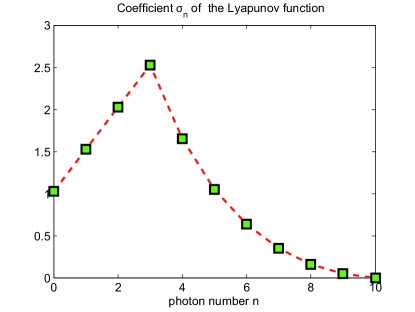
Figure 1: The coefficients $\sigma_{n}$ used for the Lyapunov function $W_{\epsilon}(\rho)$ defined in Theorem 4.1 during the closed-loop simulations, the goal photon number $\bar{n}=3$ corresponds to the maximum of the $\sigma_{n}$.

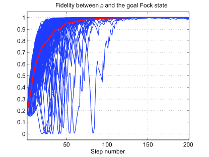
Figure 2: $\left<3\right|\rho_{k}\left|3\right>$ (Ideal case; fidelity with respect to the $3$-photon goal state) versus the time step $k\in\{0,\cdots,200\}$ for $100$ realizations of the closed-loop Markov process (blue curves) starting from the same coherent state $\rho_{0}={\mathbb{U}}_{\sqrt{3}}(\left|0\right>\left<0\right|).$ The ensemble average over these realizations corresponds to the thick red curve.

6 Concluding remarks

The method proposed here to derive strict control-Lyapunov could certainly be extended to

• prove exponential closed-loop convergence for the feedback law given by theorem 4.1.

• the general situation where the control $u$ appears directly in the Kraus operators $M_{\mu}(u)$ instead of being separated from the QND measures and attached to a unitary evolution applied after each measurement.

• continuous-time quantum systems subject to QND measurements such as those considered in [8] and described in detail in [14].

• infinite-dimensional quantum systems as in [10] that consider the photon-box system without truncation to a finite number of photons.

Appendix A Appendix

Theorem A.1.

Let $X_{k}$ be a Markov chain on the compact state space $S.$ Suppose, there exists a non-negative function $V(X)$ satisfying

$${\text{\normalsize$\mathbb{E}$}}\left(V(X_{k+1})|X_{k}\right)-V(X_{k})=Q(X_{k}),$$ (15)

where $Q(X)$ is a positif continuous function of $X,$ then the $\omega$-limit set $\Omega$ (in the sense of almost sure convergence) of $X_{k}$ is included in the following set

$$I:=\{X|\quad Q(X)=0\}.$$

Proof.

The proof is just an application of the Theorem $1$ in [6, Ch. 8], which shows that $Q(X_{k})$ converges to zero for almost all paths. It is clear that the continuity of $Q(X)$ with respect to $X$ and the compactness of $S$ implies that the $\omega$-limit set of $X_{k}$ is necessarily included into the set I. ∎

References

- [1] H. Amini, M. Mirrahimi, and P. Rouchon. Stabilization of a delayed quantum system: the Photon Box case-study. 2010. Submitted, preprint at arXiv:1007.3584v1.
- [2] L.W. Beineke and R.J. Wilson. Topics in algebraic graph theory. Cambridge University Press,, 2004.
- [3] V.B. Braginskii and Y.I. Vorontsov. Quantum-mechanical limitations in macroscopic experiments and modern experimental technique. Sov. Phys. Usp., 17(5):644–650, 1975.
- [4] I. Dotsenko, M. Mirrahimi, M. Brune, S. Haroche, J.-M. Raimond, and P. Rouchon. Quantum feedback by discrete quantum non-demolition measurements: towards on-demand generation of photon-number states. Physical Review A, 80: 013805-013813, 2009.
- [5] S. Haroche and J.M. Raimond. Exploring the Quantum: Atoms, Cavities and Photons. Oxford University Press, 2006.
- [6] H.J. Kushner. Introduction to Stochastic Control. Holt, Rinehart and Wilson, INC., 1971.
- [7] M. Mirrahimi, I. Dotsenko, and P. Rouchon. Feedback generation of quantum Fock states by discrete QND measures. In Decision and Control, 2009 held jointly with the 2009 28th Chinese Control Conference. CDC/CCC 2009. Proceedings of the 48th IEEE Conference on, pages 1451 –1456, 2009.
- [8] M. Mirrahimi and R. Van Handel. Stabilizing feedback controls for quantum systems. SIAM Journal on Control and Optimization, 46(2):445–467, 2007.
- [9] C. Sayrin, I. Dotsenko, X. Zhou, B. Peaudecerf, Th. Rybarczyk, S. Gleyzes, P. Rouchon, M. Mirrahimi, H. Amini, M. Brune, J.M. Raimond, and S. Haroche. Real-time quantum feedback prepares and stabilizes photon number states. To appear in Nature, 2011. preprint arXiv:1107.4027v1.
- [10] R. Somaraju, M. Mirrahimi, and P. Rouchon. Approximate stabilization of an infinite dimensional quantum stochastic system. In to appear in 50th IEEE Conference on Decision and Control, 2011. http://arxiv.org/abs/1103.1724.
- [11] J. Stockton, R. Van Handel, and H. Mabuchi. Deterministic Dicke-state preparation with continuous measurement and control. Physical Review A, 70(2):22106, 2004.
- [12] K.S. Thorne, R.W.P. Drever, C.M. Caves, M. Zimmermann, and V.D. Sandberg. Quantum nondemolition measurements of harmonic oscillators. Phys. Rev. Lett., 40:667–671, 1978.
- [13] W.G. Unruh. Analysis of quantum-nondemolition measurement. Phys. Rev. D, 18:1764–1772, 1978.
- [14] H.M. Wiseman and G.J. Milburn. Quantum Measurement and Control. Cambridge University Press, 2009.