Response of the polaron system consisting of an impurity in a Bose-Einstein condensate to Bragg spectroscopy

Abstract

We expand the existing polaron response theory, expressed within the Mori-Zwanzig projection operator formalism applicable for the transfer of arbitrary energy and zero momentum, to the the case of finite momentum exchange. A general formula is then derived which can be used to calculate the response of a system to a probe that transfers both momentum and energy to the system. The main extension of the existing polaron response theory is the finite momentum exchange which was not needed until now since it is negligible for optical absorption. However, this formalism is needed to calculate the response of the polaronic system consisting of an impurity in a Bose-Einstein condensate to Bragg spectroscopy. We show that the well-known features that appear in the optical absorption of the solid state Fröhlich polaron are also present in the Bragg response of the BEC-impurity polaron. The f-sum rule is written in a form suitable to provide an independent consistency test for our results. The effect of lifetime broadening on the BEC-impurity spectrum is examined. The results derived here are discussed in the framework of an experimental realization consisting of a lithium impurity in a sodium condensate.

I Introduction

The experimental realization of impurities in a Bose-Einstein condensate (BEC) CavityNature ; PhysRevLett.85.483 ; 063118 and the possibility to produce quantum degenerate atomic mixtures PhysRevLett.95.170408 ; PhysRevLett.89.190404 ; PhysRevLett.88.160401  has resulted in an interest in the physics of impurities in a quantum gas. This has led to an investigation of the change of the properties of the bare impurities as a result of the interactions with the condensate (such as the effective interaction PhysRevA.72.023616 ; PhysRevA.61.053601 and the effective mass PhysRevA.70.013608 ; girardeau:279 ; Gross1962234 ) and a study of the self-trapping of the impurity PhysRevA.73.043608 ; PhysRevB.46.301 . Also the system of a spin down fermion in a sea of spin up fermions, usually indicated as the Fermi polaron, has been investigated which resulted in a good agreement between theory PhysRevA.80.033607 ; PhysRevB.77.020408 and experiments PhysRevLett.103.170402 ; PhysRevLett.102.230402 . Furthermore it was shown that when the Bogoliubov approximation is valid the system of an impurity in a BEC can be mapped to the Fröhlich polaron system PhysRevLett.96.210401 ; PhysRevA.73.063604 ; PhysRevB.80.184504 which shows that this system can be added to the list of condensed matter systems that can be imitated in the context of quantum gases RevModPhys.80.885 . The experimental realization of quantum degenerate atomic mixtures in an optical lattice PhysRevLett.102.030408 ; PhysRevLett.96.180403 ; PhysRevLett.96.180402 has led to the theoretical study of the polaronic properties of impurities in a BEC where the influence of the optical lattice is felt only by the impurities PhysRevA.76.011605 ; 1367-2630-10-3-033015 or by both the impurities and the condensate 2010arXiv1009.0675P .

In the context of solid state physics the Fröhlich polaron consists of a charge carier (electron, hole) interacting with the phonons in an ionic crystal or a polar semiconductor LandauPekar ; Frolich3 . This Fröhlich polaron Hamiltonian can not be diagonalised exactly and several approximation methods have been developed for it. The most general way to study the system is through a variational principle within the path integral formalism which was developed by Feynman PhysRev.97.660 . The internal excitation spectrum of the Fröhlich polaron was revealed through the calculation of the optical absorption by Devreese et al. PhysRevB.5.2367 , based on the Feynman path integral method and a response formalism introduced in Ref. PhysRev.127.1004 . Recently the excitation spectrum of the Fröhlich polaron Hamiltonian was also studied numerically with Diagrammatic Quantum Monte-Carlo numerical techniques and these results showed deviations in the large coupling optical absorption linewidth with the theoretical results of PhysRevB.5.2367 , see Ref. PhysRevLett.91.236401 . At weak and intermediate coupling the analytical theory of Ref. PhysRevB.5.2367 agrees well with the numerical simulations of Ref. PhysRevLett.91.236401 and this optical absorption spectrum was also studied experimentally PhysRevB.64.104504 . So far the strong coupling regime could not be probed experimentally since the largest attainable Fröhlich polaron coupling constant in any solid is not large enough. The large coupling behavior remains an important question since a better understanding of the intermediate and strong coupling regimes might be useful to elucidate the role of polarons and bipolarons in unconventional pairing mechanisms e.g. for high-temperature superconductivity PhysRevB.77.094502 . Furthermore it was shown that at intermediate coupling the introduction of an ad hoc lifetime $\tau$ for the eigenstates of the polaron model system is an improvement of the theory which is called the extended memory function formalism PhysRevLett.96.136405 .

If the Bogoliubov approximation is applicable the Hamiltonian of an impurity in a BEC can be written as the sum of the mean field energy of the homogeneous condensate and the Fröhlich polaron Hamiltonian that describes the fluctuations PhysRevB.80.184504 :

$$\widehat{H}_{pol}=\frac{\widehat{p}^{2}}{2m_{I}}+\sum_{\vec{k}\neq 0}\hbar\omega_{\vec{k}}\widehat{b}_{\vec{k}}^{{\dagger}}\widehat{b}_{\vec{k}}+\sum_{\vec{k}\neq 0}V_{\vec{k}}e^{i\vec{k}.\widehat{r}}\left(\widehat{b}_{\vec{k}}+\widehat{b}_{-\vec{k}}^{{\dagger}}\right),$$ (1)

which describes the interaction between the impurity and the Bogoliubov excitations where $\widehat{r}$ and $\widehat{p}$ represent the position and momentum of the impurity with mass $m_{I}$, $\widehat{b}_{\vec{k}}$ and $\widehat{b}_{\vec{k}}^{{\dagger}}$ are the annihilation and creation operators for the Bogoliubov excitations, $\omega_{\vec{k}}$ is the Bogoliubov frequency:

$$\omega_{\vec{k}}=ck\sqrt{1+\left(\xi k\right)^{2}/2},$$ (2)

and $V_{\vec{k}}$ is the interaction amplitude:

$$V_{\vec{k}}=\sqrt{N_{0}}\left[\frac{\left(\xi k\right)^{2}}{\left(\xi k\right)^{2}+2}\right]^{1/4}g_{IB}.$$ (3)

In the above expressions use was made of the definition of the healing length of the condensate: $\xi=1/\sqrt{8\pi a_{BB}n_{0}}$ with $n_{0}=N_{0}/V$ the condensate density and $a_{BB}$ the boson-boson scattering length. We also used the expression for the speed of sound in the condensate: $c=\hbar/\left(\sqrt{2}m_{B}\xi\right)$. In PhysRevB.80.184504 the Feynman variational path integral technique was applied to this Hamiltonian and an upper bound for the free energy was calculated by using the Jensen-Feynman inequality with the Feynman model system. This model system consists of the impurity mass coupled to another mass $M$ by a spring with frequency $\Omega$. The parameters $M$ and $\Omega$ are then used to minimize the free energy. It followed that the Fröhlich polaron coupling parameter in this case is given by:

$$\alpha=\frac{a_{IB}^{2}}{a_{BB}\xi},$$ (4)

with $a_{IB}$ the impurity-boson scattering length. Together with the ratio between the masses of the impurity and the bosons this coupling parameter fully determines the static properties of the specific BEC-impurity polaron system. Depending on the value of this coupling strength two regimes were identified: a strong coupling regime which has properties that suggested a polaronic self-trapped state and a weak coupling regime which suggested a free polaron. Since this coupling parameter depends strongly on the scattering lengths, which can be tuned externally by a magnetic field through a Feshbach resonance (see eg. Pitaevskii ), it may be possible to tune the system experimentally to the regime of strong coupling. This technique might enable the experimental realization of the strong coupling regime and reveal the internal structure of the Fröhlich polaron Hamiltonian.

Since, as opposed to the original Fröhlich polaron in solid state, the BEC-impurity polaron system is not charged it is not helpful to perform optical absorption measurements on this system. The method to probe the system is addressed in the present paper and will be shown to be Bragg spectroscopy. This has proven to be a very succesfull tool to probe the structure of BEC’s (see eg. PhysRevLett.83.2876 and PhysRevLett.88.120407 ). It is realized by probing the system with two laser beams with wave vectors $\vec{k}_{1}$ and $\vec{k}_{2}$ and frequencies $\omega_{1}$ and $\omega_{2}$. An atom can then undergo a stimulated scattering event by absorbing a photon from beam 1 and emitting it in beam 2 which changes its momentum by $\vec{k}=\vec{k}_{1}-\vec{k}_{2}$ and its energy by $\hbar\omega=\hbar\omega_{1}-\hbar\omega_{2}$. See figure 1 for a schematical picture of a typical experimental set-up. A possible way to measure the response of the system is by performing a time-of-flight experiment and count the number of atoms $N_{Bragg}$ that have gained a momentum $\vec{k}$. Within the formalism of linear response theory this number is given by Pitaevskii :

$$N_{Bragg}=\frac{2}{\hbar}\left(\frac{V}{2}\right)^{2}\tau\operatorname{Im}\chi\left(\omega,\vec{k}\right),$$ (5)

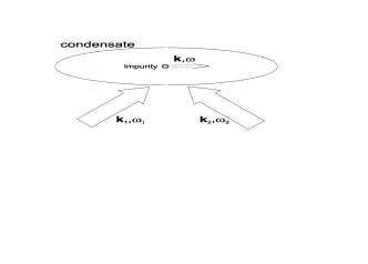
Figure 1: Schematical picture of a typical experimental set-up for Bragg spectroscopy. Two lasers with momentum $\vec{k}_{1}$ and $\vec{k}_{2}$ and energy $\hbar\omega_{1}$ and $\hbar\omega_{2}$ are impinged upon the impurity in the condensate which gains an energy $\hbar\omega=\hbar\omega_{1}-\hbar\omega_{2}$ and a momentum $\vec{k}=\vec{k}_{1}-\vec{k}_{2}.$

with $\tau$ the duration of the pulse, $V$ the amplitude of the laser induced potential and $\chi\left(\omega,\vec{k}\right)$ the density response function, defined by:

$$\chi\left(\omega,\vec{k}\right)=-\frac{1}{\hbar}\mathcal{Z}^{-1}\sum_{m,n}e^{-\beta E_{m}}\left[\frac{\left|\left\langle m\left|\rho_{\vec{k}}\right|n\right\rangle\right|^{2}}{\omega-\omega_{nm}+i\delta}-\frac{\left|\left\langle m\left|\rho_{\vec{k}}^{{\dagger}}\right|n\right\rangle\right|^{2}}{\omega+\omega_{nm}+i\delta}\right],$$ (6)

with $\rho_{\vec{k}}$ the induced density of the impurity, $\mathcal{Z}$ the partition function, $|n>$ the eigenstates of the unperturbed system and $\omega_{nm}=\left(E_{n}-E_{m}\right)/\hbar$ the transition frequencies. This density response function can be rewritten as the Fourier transform of the retarded density-density correlation function:

$$\chi\left(\omega,\vec{k}\right)=\frac{i}{\hbar}\int_{0}^{\infty}dte^{i\omega t}\left\langle\left[\rho_{\vec{k}}\left(t\right),\rho_{\vec{k}}^{{\dagger}}\right]\right\rangle.$$ (7)

The retarded density-density correlation function is needed to obtain the response of a system to Bragg spectroscopy.

We will start by using the Mori formalism to calculate a general expression for the density-density correlation function (7) and then apply it to the generic polaron system with arbitrary dispersion and interaction amplitude. Then we show that if we calculate from this expression the current-current correlation for the $\vec{k}=0$ limit we find the known result for the optical absorption of Ref. PhysRevB.5.2367 . Next we introduce the dispersion and interaction amplitude for the BEC-impurity polaron and obtain results for the response to Bragg spectroscopy. The result is expressed as a double integral over highly oscillatory integrands that has to be calculated numerically and which can give numerical problems. To overcome these problems we will then rewrite our expressions in another representation which is suitable for numerical work. We then write down the f-sum rule to check our results and find that at low temperature there is a relatively large recoil contribution for $\omega\rightarrow 0$ which numerically has to be added separately in the sum rule. This behavior was also found in the optical absorption of the solid state Fröhlich polaron and in that case there is a relation with the effective mass of the polaron PhysRevB.15.1212 . Recently this sum rule was used to experimentally determine the effective mass of the solid state Fröhlich polaron, see Refs. PhysRevLett.100.226403 and PhysRevB.81.125119 . Next, following De Filippis et al PhysRevLett.96.136405 , we introduce a lifetime $\tau$ and examine the dependence of the theory on this lifetime. The results are analyzed for the experimental setup consisting of a Lithium impurity in a sodium condensate which is the same system that was examined in Ref. PhysRevB.80.184504 .

II Application of the Mori formalism to the density-density correlation

The Mori-Zwanzig projection operator technique (see PTP.33.423 and PhysRev.124.983 ) is a well established technique to calculate correlation functions and has been applied before to the Fröhlich polaron Hamiltonian to calculate the optical absorption by Peeters and Devreese PhysRevB.28.6051 (for a detailed description we refer to ZomerschoolDevreese ) . This technique can also be applied to the calculation of the density-density correlation function. There is however one obstacle that we encountered when defining the Mori projection operator. The reason is that the common definition of this operator is ill-defined since it leads to a vanishing density-density commutator. This problem was already noticed by Ichiyanagi JPSJ.32.604 and he suggested the following definition for the action of the Mori projection operator $P$ on an arbitrary operator $A$:

$$PA=\frac{\left\langle\left[A,\dot{\rho}_{\vec{k}}^{{\dagger}}\right]\right\rangle}{\left\langle\left[\rho_{\vec{k}},\dot{\rho}_{\vec{k}}^{{\dagger}}\right]\right\rangle}\rho_{\vec{k}}.$$ (8)

In our calculations we have followed this suggestion and found that the density response function can be written as:

$$\chi\left(\omega,\vec{k}\right)=\frac{i}{\hbar}\frac{\varphi}{\omega^{2}+O-\Sigma\left(\omega,\vec{k}\right)},$$ (9)

with:

$$\varphi =\left\langle\left[\rho_{\vec{k}},\dot{\rho}_{\vec{k}}^{{\dagger}}\right]\right\rangle;$$ (10)

$$O =\frac{\omega}{\varphi}\left\langle\left[L\rho_{\vec{k}},\dot{\rho}_{\vec{k}}^{{\dagger}}\right]\right\rangle;$$ (11)

$$\Sigma\left(\omega,\vec{k}\right) =-\frac{1}{\varphi}\int_{0}^{\infty}dt\left(1-e^{i\omega t}\right)\left\langle\left[\mathcal{B}_{\vec{k}}\left(t\right),\mathcal{B}_{\vec{k}}^{{\dagger}}\right]\right\rangle.$$ (12)

Where $L$ is the Liouville operator and $\Sigma\left(\omega,\vec{k}\right)$ is known as the memory function or self energy. Furthermore we also introduced the operator $\mathcal{B}_{\vec{k}}\left(t\right)$ defined as:

$$\mathcal{B}_{\vec{k}}=QL\dot{\rho}_{\vec{k}},$$ (13)

with $Q$ the complementary Mori projection operator: $Q=1-P$. The time dependence of $\mathcal{B}_{\vec{k}}\left(t\right)$ is governed by a new Liouville operator defined by $\mathcal{L=}QLQ$. It is important to note here that until this point no approximations were made and the result (9) for the linear density response function is exact. Also, to derive the formula (9) we have not introduced a specific system and so it is a general result for the density response function and can also be applied to calculate the response of other systems to probes with an arbitrary energy and momentum exchange. For example the final state of neutron scattering is also determined by the density reponse function PhysRev.95.249 . We now consider the Fröhlich polaron Hamiltonian and follow an approach similar to that used in Ref. PhysRevB.28.6051 . This consists in replacing the new Liouville operator $\mathcal{L}$ by the sum of the Liouville operator of free Bogoliubov excitations $L_{Bog}$ and the Liouville operator of the Feynman modelsystem $L_{F}$: $\mathcal{L\rightarrow}L_{Bog}+L_{F}$. Within this approximation we can calculate the different quantities in the expression (9) which gives $O=0$ and:

$$\varphi=i\frac{\hbar k^{2}}{m_{I}}N,$$ (14)

where $N$ is the number of impurities. The memory function is then given by:

$$\Sigma\left(\omega,\vec{k}\right) =\frac{2}{m_{I}N\hbar}\sum_{\vec{q}\neq 0}\left|V_{\vec{q}}\right|^{2}\frac{\left(\vec{k}.\vec{q}\right)^{2}}{k^{2}}\int_{0}^{\infty}dt\left(1-e^{i\omega t}\right)$$

$$\times\operatorname{Im}\left\{\left[e^{i\omega_{\vec{q}}t}+2\cos\left(\omega_{\vec{q}}t\right)n_{\vec{q}}\right]\exp\left[-\left(\vec{k}+\vec{q}\right)^{2}D\left(t\right)\right]\right\},$$ (15)

with $n_{\vec{q}}$ the Bose-Einstein distrubution, i.e. the number of Bogoliubov excitations with frequency $\omega_{\vec{q}}$ and $D\left(t\right)$ describes the Feynman model system and is given by:

$$D\left(t\right) =\frac{t^{2}}{2\beta\left(m+M\right)}-i\frac{\hbar}{2\left(m+M\right)}t$$

$$+\frac{\hbar M}{2m\Omega(m+M)}\left(1-\exp\left(i\Omega t\right)+4\sin^{2}\left(\frac{\Omega t}{2}\right)n\left(\Omega\right)\right),$$ (16)

with $M$ and $\Omega$ the variational parameters. The values of these parameters are deduced from the minimalisation of the free energy PhysRevB.80.184504 .

III Link with the optical absorption of the solid state Fröhlich polaron

A well-known result from linear response theory and the Kubo formalism is that the optical absorption of a system can be expressed as a current-current correlation function Mahan . Since the current and the density are related to each other through the continuity equation it is possible to calculate the current-current correlation function from the density-density correlation function. For the process of optical absorption the photon momentum is negligible in comparison to the other momenta involved in the polaron problem, which is not the case for Bragg spectroscopy. To obtain the optical absorption we have to take the limit $\vec{k}\rightarrow 0$ which gives for the memory function:

$$\Sigma\left(\omega,0\right) =\frac{2}{3m_{I}N\hbar}\sum_{\vec{q}\neq 0}\left|V_{\vec{q}}\right|^{2}q^{2}\int_{0}^{\infty}dt\left(1-e^{i\omega t}\right)$$

$$\times\operatorname{Im}\left\{\left[e^{i\omega_{\vec{q}}t}+2\cos\left(\omega_{\vec{q}}t\right)n_{\vec{q}}\right]\exp\left[-q^{2}D\left(t\right)\right]\right\}.$$ (17)

This is just the memory function $\Sigma\left(\omega\right)$ calculated in Ref. PhysRevB.28.6051 multiplied by $\omega$:

$$\Sigma\left(\omega,0\right)=\omega\Sigma\left(\omega\right).$$ (18)

For the solid state Fröhlich polaron it is the current-current correlation that is needed for the optical absorption. By applying two partial integrations and making use of the continuity equation one can find a simple relation between the two:

$$\chi\left(\omega,\vec{k}\right)=-\frac{i}{\hbar\omega^{2}}\int_{0}^{\infty}dte^{i\omega t}\left\langle\left[\vec{k}.\vec{j}_{\vec{k}}\left(t\right),\vec{k}.\vec{j}_{\vec{k}}^{{\dagger}}\right]\right\rangle$$ (19)

We now make use of the standard Kubo formula for the optical conductivity (see e.g. Mahan ):

$$\operatorname{Re}\left[\sigma\left(\omega\right)\right] =\operatorname{Re}\left[i\frac{e^{2}}{Vm\omega}+\frac{1}{\hbar\omega}\int_{0}^{\infty}dte^{i\omega t}\left\langle\left[j_{x}\left(t\right),j_{x}\right]\right\rangle\right]$$

$$=\lim_{\vec{k}\rightarrow 0}\operatorname{Im}\left[-\frac{\hbar\omega}{k^{2}}\chi\left(\omega,\vec{k}\right)\right]$$

$$=\operatorname{Im}\left[-\frac{1}{m_{I}}\frac{1}{\omega-\Sigma\left(\omega\right)}\right],$$ (20)

this is the result that was found in Ref. PhysRevB.5.2367  from the Feynman path integral formalism and rederived in Ref. PhysRevB.28.6051 using Mori’s formalism.

IV Results for the BEC-impurity polaron

In this section we will introduce the dispersion and the interaction amplitude for the BEC-impurity system and obtain an expression for the response of the system to a Bragg pulse. From expression (5) it follows that the response of the system is characterised by the imaginary part of the density response function which can be written as:

$$\operatorname{Im}\left[\chi\left(\omega,\vec{k}\right)\right]=-\frac{k^{2}}{m_{I}}N\frac{\operatorname{Im}\left[\Sigma\left(\omega,\vec{k}\right)\right]}{\left(\omega^{2}-\operatorname{Re}\left[\Sigma\left(\omega,\vec{k}\right)\right]\right)^{2}+\left(\operatorname{Im}\left[\Sigma\left(\omega,\vec{k}\right)\right]\right)^{2}}.$$ (21)

This particular form for the response function is general for the Fröhlich polaron and was first introduced in PhysRevB.5.2367 . The memory function for the BEC-impurity system is given by (with polaronic units i.e. $\hbar=m_{I}=\xi=1$):

$$\Sigma\left(\omega,\vec{k}\right) =\frac{1}{N}\frac{\alpha}{4\pi}\left(\frac{m_{B}+1}{m_{B}}\right)^{2}\int_{0}^{\infty}dq\frac{q^{5}}{\sqrt{q+2}}\int_{0}^{\infty}d\widetilde{t}\left(1-e^{i\omega t}\right)$$

$$\times\operatorname{Im}\left[\frac{\left[e^{i\omega_{\vec{q}}t}+2\cos\left(\omega_{\vec{q}}t\right)n_{\vec{q}}\right]}{\left[2kqD\left(t\right)\right]^{3}}\left(\exp\left[-\left(k-q\right)^{2}D\left(t\right)\right]\left\{\left[1-2kqD\left(t\right)\right]^{2}+1\right\}\right.\right.$$

$$\left.\left.-\exp\left[-\left(k+q\right)^{2}D\left(t\right)\right]\left\{\left[1+2kqD\left(t\right)\right]^{2}+1\right\}\right)\right].$$ (22)

The double integral in expression (22) could not be calculated analytically and it was computed numerically.

V Second representation for the imaginary part of the memory function

Due to the highly oscillatory behavior of the integrand it turns out that expression (22) is not of a form efficient for numerical calculation of the imaginary part of the memory function. Therefore we develop an alternative representation for the memory function which allows to perform the time integration analytically. This provides a representation for the imaginary part that is well-suited for numerical calculations. The real part of the memory function turns out to be far more involved but it seems that in this case we can use expression (22). We will follow a similar approach as was used in Ref. PhysRevB.5.2367 and also in Ref. PhysRevB.28.6051 . We start by rewriting (16) as:

$$D\left(t\right) =\frac{t^{2}}{2\beta\left(m+M\right)}-i\frac{\hbar}{2\left(m+M\right)}t$$

$$+\frac{\hbar M}{2m\Omega(m+M)}\left[\coth\left[\frac{\hbar\beta\Omega}{2}\right]-\left(1+n\left(\Omega\right)\right)\exp\left(i\Omega t\right)-n\left(\Omega\right)\exp\left(-i\Omega t\right)\right].$$ (23)

After two Taylor expansions for the two exponentials and writing the term with $t^{2}$ as a Gaussian integral we obtain:

$$\exp\left(-\left(\vec{k}+\vec{q}\right)^{2}D\left(t\right)\right) =\left(\frac{\beta}{2\pi\left(m+M\right)}\right)^{1/2}e^{-\left(\vec{k}+\vec{q}\right)^{2}\frac{\hbar M}{2m\Omega(m+M)}\coth\left[\frac{\hbar\beta\Omega}{2}\right]}$$

$$\times\sum_{n,n^{\prime}}^{\infty}\frac{1}{n!}\frac{1}{n^{\prime}!}\left[\frac{\hbar M}{2m\Omega(m+M)}\left(1+n\left(\Omega\right)\right)\right]^{n}\left[\frac{\hbar M}{2m\Omega(m+M)}n\left(\Omega\right)\right]^{n^{\prime}}$$

$$\times\left(\vec{k}+\vec{q}\right)^{2\left(n+n^{\prime}\right)}\int_{-\infty}^{\infty}dp\exp\left\{-\frac{\beta p^{2}}{2\left(M+m\right)}\right\}$$

$$\times\exp\left\{it\left[\frac{\hbar\left(\vec{k}+\vec{q}\right)^{2}}{2\left(m+M\right)}\pm\frac{p\left|\vec{k}+\vec{q}\right|}{m+M}+\left(n-n^{\prime}\right)\Omega\right]\right\}.$$ (24)

Furthermore the memory function can be written as:

$$\Sigma\left(\omega,\vec{k}\right) =\frac{\hbar\omega}{\chi}\int_{0}^{\infty}dte^{i\omega t}\int_{0}^{\beta}d\lambda\left\langle\mathcal{B}_{\vec{k}}\left(t-i\hbar\lambda\right)\mathcal{B}_{\vec{k}}^{{\dagger}}\right\rangle$$

$$=-\frac{i\omega}{Nm}\sum_{\vec{q}\neq 0}\left|V_{\vec{q}}\right|^{2}\frac{\left(\vec{k}.\vec{q}\right)^{2}}{k^{2}}\int_{0}^{\infty}dte^{i\omega t}\int_{0}^{\beta}d\lambda\left[\left(1+n_{\vec{q}}\right)e^{-i\omega_{\vec{q}}\left(t-i\hbar\lambda\right)}+n_{\vec{q}}e^{i\omega_{\vec{q}}\left(t-i\hbar\lambda\right)}\right]$$

$$\times\exp\left[-\left(\vec{k}+\vec{q}\right)^{2}D\left(-t+i\hbar\lambda\right)\right].$$ (25)

Now the time integration is straightforward:

$$\Sigma\left(\omega,\vec{k}\right) =\frac{\omega}{Nm}\left(\frac{\beta}{2\pi\left(m+M\right)}\right)^{1/2}\sum_{\vec{q}\neq 0}\left|V_{\vec{q}}\right|^{2}e^{-\left(\vec{k}+\vec{q}\right)^{2}a^{2}\left(\beta\right)}\frac{\left(\vec{k}.\vec{q}\right)^{2}}{k^{2}}\sum_{n,n^{\prime}}^{\infty}B\left(\beta,n,n^{\prime}\right)$$

$$\times\left(\vec{k}+\vec{q}\right)^{2\left(n+n^{\prime}\right)}\int_{-\infty}^{\infty}dpe^{-\frac{\beta p^{2}}{2\left(M+m\right)}}\left[\frac{1-e^{-\hbar\beta\nu_{-}}}{\hbar\nu_{-}}\frac{n_{\vec{q}}}{\omega-\nu_{-}+i\varepsilon}+\frac{1-e^{-\hbar\beta\nu_{+}}}{\hbar\nu_{+}}\frac{1+n_{\vec{q}}}{\omega-\nu_{+}+i\varepsilon}\right],$$ (26)

with the following notation:

$$a^{2}\left(\beta\right) =\frac{\hbar M}{2m\Omega(m+M)}\coth\left[\frac{\hbar\beta\Omega}{2}\right];$$ (27)

$$B\left(\beta,n,n^{\prime}\right) =\frac{1}{n!}\frac{1}{n^{\prime}!}\left[a^{2}\left(1+n\left(\Omega\right)\right)\right]^{n}\left[a^{2}n\left(\Omega\right)\right]^{n^{\prime}};$$ (28)

$$\nu_{\pm} =\pm\omega_{\vec{q}}+\frac{\hbar\left(\vec{k}+\vec{q}\right)^{2}}{2\left(m+M\right)}\pm\frac{p\left|\vec{k}+\vec{q}\right|}{m+M}+\left(n-n^{\prime}\right)\Omega.$$ (29)

The memory function is now split in an imaginary and a real part with the formula of Plemelj. The integral over $p$ in the imaginary part of (26) can be performed easily by using the delta function. Taking into account the dispersion and the interaction amplitude, this yields (with polaronic units):

$$\operatorname{Im}\left[\Sigma\left(\omega,\vec{k}\right)\right] =-\frac{1}{N}\frac{\alpha}{8}\left(\frac{m_{B}+1}{m_{B}}\right)^{2}\left(\frac{\beta\left(1+M\right)}{2\pi}\right)^{1/2}$$

$$\times\int_{0}^{\infty}dqq^{2}\int_{-1}^{1}dx\sqrt{\frac{q^{2}}{q^{2}+2}}e^{-\left(k^{2}+q^{2}+2qkx\right)a^{2}\left(\beta\right)}\left(qx\right)^{2}$$

$$\times\sum_{n,n^{\prime}}^{\infty}B\left(\beta,n,n^{\prime}\right)\left(k^{2}+q^{2}+2qkx\right)^{\left(n+n^{\prime}\right)-1/2}\left(1-e^{-\beta\omega}\right)$$

$$\times\left[n_{\vec{q}}\exp\left\{-\frac{\beta\left(M+1\right)A_{n}^{-}\left(\omega\right)^{2}}{2\left(k^{2}+q^{2}+2qkx\right)}\right\}+\left(1+n_{\vec{q}}\right)\exp\left\{-\frac{\beta\left(M+1\right)A_{n}^{+}\left(\omega\right)^{2}}{2\left(k^{2}+q^{2}+2qkx\right)}\right\}\right],$$ (30)

with:

$$A_{n}^{\pm}\left(\omega\right)=\pm\omega_{\vec{q}}+\frac{\left(\vec{k}+\vec{q}\right)^{2}}{2\left(1+M\right)}+\left(n-n^{\prime}\right)\Omega-\omega.$$

As shown in Ref. PhysRevB.28.6051 this expression has a very natural interpretation: every term in the double sum corresponds to a well-defined physical process. The ($n$,$n^{\prime}$)th term in the summation represents a scattering process of the polaron where in the initial state the polaron is in the $n^{\prime}$th internal Franck-Condon state of the Feynman polaron model system and is then scattered to the $n$th internal Franck-Condon state with the absorption of an energy $\hbar\omega$ and a momentum $\vec{k}$ through the Bragg scattering and with the emission (or absorption) of a Bogoliubov excitation with energy $\hbar\omega_{\vec{q}}$.

VI Sum rule

As a consistency check of our results we can apply the f-sum rule to our results, this can be written as:

$$\int_{0}^{\infty}d\omega\omega\operatorname{Im}\left[\chi\left(\omega,\vec{k}\right)\right]=N\frac{\pi}{2}\frac{k^{2}}{m_{I}}.$$ (31)

At small $\omega$ and as temperature tends to zero a delta peak appears in the integrand for which, in numerical calculations, we have to add the contribution separately. This feature was found for the solid state Fröhlich polaron, where the contribution of the delta peak can be used to determine the effective mass of the polaron PhysRevB.15.1212 . The delta peak can be revealed if we look at the $\omega\rightarrow 0$ limits of the imaginary and real part of expression (22) for the memory function:

$$\lim_{\omega\rightarrow 0}\operatorname{Im}\left[\Sigma\left(\omega,\vec{k}\right)\right] =0;$$ (32)

$$\lim_{\omega\rightarrow 0}\frac{\operatorname{Re}\left[\Sigma\left(\omega,\vec{k}\right)\right]}{\omega^{2}} =R\left(\alpha,\vec{k}\right),$$ (33)

with:

$$R\left(\alpha,\vec{k}\right) =\frac{\omega_{0}^{2}}{N}\frac{\alpha}{4\pi}\left(\frac{m_{B}+1}{m_{B}}\right)^{2}\int_{0}^{\infty}d\widetilde{q}\widetilde{q}^{2}\frac{q}{\sqrt{q+2}}q^{2}\int_{0}^{\infty}dt\frac{t^{2}}{2}$$

$$\times\operatorname{Im}\left[\frac{\left[e^{i\omega_{\vec{q}}t}+2\cos\left(\omega_{\vec{q}}t\right)n_{\vec{q}}\right]}{\left[2kqD\left(t\right)\right]^{3}}\left(\exp\left[-\left(k-q\right)^{2}D\left(t\right)\right]\left\{\left[1-2kqD\left(t\right)\right]^{2}+1\right\}\right.\right.$$

$$\left.\left.-\exp\left[-\left(k+q\right)^{2}D\left(t\right)\right]\left\{\left[1+2kqD\left(t\right)\right]^{2}+1\right\}\right)\right].$$ (34)

If we now look at the $\omega\rightarrow 0$ limit of the density response function we find:

$$\lim_{\omega\rightarrow 0}\operatorname{Im}\left[\chi\left(\omega,\vec{k}\right)\right]=\frac{k^{2}N}{m_{I}\left(1-R\left(\alpha\right)\right)}\pi\delta\left(\omega^{2}\right),$$ (35)

where we used the following representation for the delta function:

$$\delta\left(x\right)=\lim_{n\rightarrow 0}\frac{1}{n\pi}\frac{1}{1+\left(x/n\right)^{2}}.$$ (36)

So at temperature zero the sum rule becomes:

$$\frac{\pi}{2}\frac{k^{2}N}{m_{I}\left(1-R\left(\alpha,\vec{k}\right)\right)}+\int_{\varepsilon}^{\infty}d\omega\omega\operatorname{Im}\left[\chi\left(\omega,\vec{k}\right)\right]=N\frac{\pi}{2}\frac{k^{2}}{m_{I}},$$ (37)

where $\varepsilon$ is a positive infinitesimal. Care has to be taken at finite temperature since the delta peak will then broaden and start to overlap with other contributions of the spectrum. At low enough temperatures we will see that our results agree well with (37).

VII Extended memory function formalism

It was noticed in Ref. Cataudella that the Feynman polaron model system does not satisfy the sum rule for the density-density correlation. This limitation can be removed by introducing a finite lifetime $\tau$ for the eigenstates of the Feynman model system which mimics scattering events with the bosonic bath, which can be done by replacing $\exp\left(i\Omega t\right)$ by $\left(1+it/\tau\right)^{\Omega\tau}$ in (16). This technique is called the extended memory function formalism and was applied in Ref. PhysRevLett.96.136405 for the solid state Fröhlich polaron. It was shown that at intermediate coupling this gives a better agreement between the theory and the Diagrammatic Quantum Monte-Carlo numerical techniques. This extension also solves the problem of the inconsistency of the linewidths at strong coupling with the uncertainty relation for the solid state Fröhlich polaron, which was first mentioned in Ref. PhysRevB.5.2367 . It seems that the second representation for the imaginary part of the memory function (30) is not suitable for the introduction of a lifetime. To obtain a qualitatively picture of the dependence of the results on the lifetime we can work with the real and imaginary part of the memory function as expressed in equation (22).

VIII Results and discussion

The results we obtain in this section are for a system consisting of a sodium condensate with a single lithium impurity, this means that we use for the bosonic mass: $m_{B}=3.8221$, which is in polaronic units as are all the results in this section.

We begin by looking at the weak coupling regime. In figure 2 the Bragg response (21) is presented as a function of the transferred energy $\hbar\omega$ for different temperatures and for a momentum exchange $k=1$. At low temperature ($\beta=100$) we clearly see a peak that represents the weak coupling scattering process and can be understood as the emission of Bogoliubov excitations. Also the contribution of the temperature broadened delta peak at low $\omega$ is seen. This is the anomalous Drude peak (see Ref. Devreese1998309 ). If we look at higher temperatures the zero temperature delta peak broadens and there is a larger overlap with the weak coupling scattering peak. At $\beta=10$ this peak has become indistinguishable from the anomalous Drude peak. For $\beta=100$ a distinction between the two contributions can still be made and the f-sum rule can be applied, as will be done below.

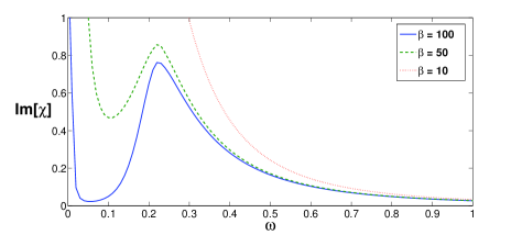
Figure 2: The Bragg response of the polaron system consisting of an impurity in a BEC polaron in the weak coupling regime ($\alpha=0.1$) with momentum exchange $k=1$ for different temperatures.

The dependence of the spectrum on the exchanged momentum $k$ is presented in figure 3 for $\alpha=0.1$ and $\beta=100$. For larger momentum exchange the scattering peak is shifted to higher frequencies and a broadening is observed. The inset of figure 3 shows the frequencies $\omega_{\max}$ at which the maximum of the peak occurs as a function of the exchanged momentum $k$ together with a least square fit to the Bogoliubov spectrum:

$$\omega=\frac{k}{2m}\sqrt{k^{2}+2},$$ (38)

where $m$ is determined as a fitting parameter to be: $m=3.9534$; which is in good agreement with the bosonic mass of the condensate ($m_{B}=3.8221$). This shift according to the Bogoliubov dispersion is plausible since the peak corresponds to the emission of Bogoliubov excitations.

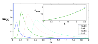
Figure 3: The Bragg response of the polaron system consisting of an impurity in a BEC in the weak coupling regime ($\alpha=0.1$) at temperature $\beta=100$ for different momentum exchanges. The inset shows the frequency og the maximum as a function of the exchanged momentum $k$. The curve gives a least square fit of the Bogoliubov spectrum (38), with fitting parameter $m=3.9534$.

In figure 4 the high frequency tail of the Bragg spectrum is shown for different coupling strengths $\alpha$ at $\beta=100$ and $k=1$. In the strong coupling regime a resonance is seen which is absent in the weak coupling regime. This feature is well-known from the solid state Fröhlich polaron and corresponds to a transition to the Relaxed Excited State (RES); it was first proposed in PhysRevLett.22.94 . This resonance appears at a frequency $\omega_{RES}$ such that $\omega_{RES}^{2}=\operatorname{Re}\left[\Sigma\left(\omega_{RES},\vec{k}\right)\right]$ with the supplementary condition $\operatorname{Im}\left[\Sigma\left(\omega_{RES},\vec{k}\right)\right]\ll 1$. It is clear from (21) that these conditions cause a peak in the spectrum. This resonance corresponds to a transition from the polaron ground state to an excited state in the polaronic self-trapping potential which has been relaxed consistent with the new excited wave function of the impurity. The coupling strength where the relaxed excited state appears in the Bragg spectrum is slightly below $\alpha=4$. This is in agreement with the prediction in PhysRevB.80.184504 that for a BEC-impurity the transition between the weak and the strong coupling regime occurs around $\alpha\simeq 3$ for $\beta\rightarrow\infty$. In the strong coupling regime other peaks are present which are indicated for $\alpha=8$ in the inset of figure 4. These are the Franck-Condon (FC) peaks and represent a transition to the RES together with the emission of Bogoliubov excitations. They only appear in the strong coupling regime which was also observed in the case of the acoustic polaron PhysRevB.35.3745 .

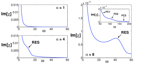
Figure 4: The Bragg response of the polaron system consisting of an impurity in a BEC at different values for the coupling parameter $\alpha$ at temperature $\beta=100$ and a momentum exchange $k=1$. In the strong coupling regime the imprint of the Relaxed Excited State resonance appears. The inset shows the first three Franck-Condon peaks at $\alpha=8$.

The dependence of the RES peak on the exchanged momentum is depicted in figure 5. The inset shows the frequency of the maximum of the RES peaks as a function of the exchanged momentum $q$ together with a least square fit to a quadratic dispersion:

$$\omega=\nu+\frac{k^{2}}{2m^{\ast}},$$ (39)

where $\nu$ and $m^{\ast}$ are the fitting parameters. This suggests that the RES  is characterized by a transition frequency $\nu$ and an effective mass $m^{\ast}$.

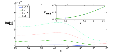
Figure 5: The Realaxed Excited State peak in the Bragg response of the polaron system consisting of an impurity in a BEC in the strong coupling regime ($\alpha=8$) at temperature $\beta=100$ for different momentum exchanges. The inset shows the frequency of the maximum as a function of the exchanged momentum $k$ at $\beta=100$. The curve is a least square fit to the quadratic dispersion (39), with fitting parameters $\nu=40.76$ and $m^{\ast}=3.84$.

As a consistency test it was checked whether the above results satisfy the f-sum rule (37). Filling out the expression for the imaginary part of the density response function (21) and dividing by the common factor the f-sum rule takes the form:

$$\frac{\pi}{2\left(1-R\left(\alpha,\vec{k}\right)\right)}-\int_{\varepsilon}^{\infty}d\omega\omega\frac{\operatorname{Im}\left[\Sigma\left(\omega,\vec{k}\right)\right]}{\left(\omega^{2}-\operatorname{Re}\left[\Sigma\left(\omega,\vec{k}\right)\right]\right)^{2}+\left(\operatorname{Im}\left[\Sigma\left(\omega,\vec{k}\right)\right]\right)^{2}}=\frac{\pi}{2}.$$ (40)

It is impossible to integrate numerically to infinity and for this reason a cut-off, $\omega_{c}=500$, is used. A calculation of the left hand side of (40) results in the values in table 1 for different values of $\alpha$ and $k$ at $\beta=100$. These results should be compared with the rigourous value $\pi/2=1.5708...$ which gives a good agreement with small deviations.

$k$	$\alpha=$	$1$	$4$	$8$
$1$		$1.5442$	$1.6845$	$1.5532$
$3$		$1.5482$	$1.6419$	$1.5355$
$5$		$1.5506$	$1.5555$	$1.4979$

Table 1: Results of a numerical calculation of the left hand side of expression (40) with a cut-off $\omega_{c}=500$ introduced for the $\omega$-integral.

We now give a qualitative analysis of the dependence of the results on the lifetime $\tau$, which was introduced in section VII within the extended memory function formalism. In figure 6 the Relaxed Excited State peak is presented at different values for $\tau$ in the strong coupling regime ($\alpha=8$). It is observed that the inclusion of a lifetime parameter of the order of the polaronic time unit results in a broadening of the peak, where a smaller lifetime corresponds to a broader peak. When a lifetime of the order of a hundredth of the polaronic time unit is introduced the peak can not be distinguished any more.

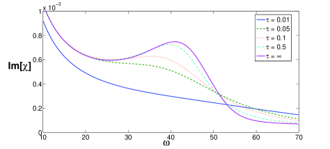
Figure 6: The Relaxed Excited State peak in the Bragg response of the polaron system consisting of an impurity in a BEC in the strong coupling regime ($\alpha=8$) at temperature $\beta=100$ with different lifetimes $\tau$.

IX Conclusions

We have derived a general formula for the density response function as a function of the transferred energy and momentum with the Mori-Zwanzig projection operator formalism. This provides a general result that can be used for Bragg spectroscopy but also for other probes that exhibit an arbitrary energy and momentum exchange as for example neutron scattering where the output is also determined by the density response function PhysRev.95.249 . This is applied to the Fröhlich polaron Hamiltonian for which the well-known results from Ref. PhysRevB.5.2367 for the optical absorption are found. We then extend the analysis to Bragg scattering of impurity polarons in a Bose condensed gas, where the Bogoliubov excitations play the role of the phonons in the polaron formation. The f-sum rule is checked.

To analyze the results we introduced the specific system of a lithium impurity in a sodium condensate and calculated the spectra in the different coupling regimes and for different momentum exchanges and temperatures. It is seen that these spectra possess similar features as also found in the optical absorption of the solid state Fröhlich polaron. Furthermore it was shown that the weak coupling scattering peaks follow the Bogoliubov spectrum as a function of the exchanged momentum. In the strong coupling regime the Relaxed Excited State emerges, and we derive the transition frequency and the effective mass associated with the Relaxed Excited State. This is of importance for the comparison with Diagrammatic Quantum Monte-Carlo numerical techniques, which in the case of the optical absorption of the solid state Fröhlich polaron has led to new results concerning the linewidth and oscillator strength of the Relaxed Excited State and Franck-Condon transitions. The Franck-Condon peaks were also observed.

Our results were tested using the f-sum rule which resulted in a good agreement with small deviations.

The influence of the introduction of a lifetime within the extended memory function formalism was also qualitatively investigated and it was shown that this results in a broadening of the RES peak.

- (1) F. Brennecke, et al., Nature 450, 268 (2007).
- (2) A. P. Chikkatur, et al., Phys. Rev. Lett. 85, 483 (2000).
- (3) A. Öttl, S. Ritter, M. Köhl, T. Esslinger, Rev. Sci. Instr. 77, 063118 (2006).
- (4) C. Silber, et al., Phys. Rev. Lett. 95, 170408 (2005).
- (5) G. Modugno, M. Modugno, F. Riboli, G. Roati, M. Inguscio, Phys. Rev. Lett. 89, 190404 (2002).
- (6) Z. Hadzibabic, et al., Phys. Rev. Lett. 88, 160401 (2002).
- (7) A. Recati, J. N. Fuchs, C. S. Peça, W. Zwerger, Phys. Rev. A 72, 023616 (2005).
- (8) M. J. Bijlsma, B. A. Heringa, H. T. C. Stoof, Phys. Rev. A 61, 053601 (2000).
- (9) G. E. Astrakharchik, L. P. Pitaevskii, Phys. Rev. A 70, 013608 (2004).
- (10) M. Girardeau, Physics of Fluids 4, 279 (1961).
- (11) E. P. Gross, Annals of Physics 19, 234 (1962).
- (12) R. M. Kalas, D. Blume, Phys. Rev. A 73, 043608 (2006).
- (13) D. K. K. Lee, J. M. F. Gunn, Phys. Rev. B 46, 301 (1992).
- (14) C. Mora, F. Chevy, Phys. Rev. A 80, 033607 (2009).
- (15) N. Prokof’ev, B. Svistunov, Phys. Rev. B 77, 020408 (2008).
- (16) S. Nascimbène, et al., Phys. Rev. Lett. 103, 170402 (2009).
- (17) A. Schirotzek, C.-H. Wu, A. Sommer, M. W. Zwierlein, Phys. Rev. Lett. 102, 230402 (2009).
- (18) F. M. Cucchietti, E. Timmermans, Phys. Rev. Lett. 96, 210401 (2006).
- (19) K. Sacha, E. Timmermans, Phys. Rev. A 73, 063604 (2006).
- (20) J. Tempere, et al., Phys. Rev. B 80, 184504 (2009).
- (21) I. Bloch, J. Dalibard, W. Zwerger, Rev. Mod. Phys. 80, 885 (2008).
- (22) T. Best, et al., Phys. Rev. Lett. 102, 030408 (2009).
- (23) S. Ospelkaus, et al., Phys. Rev. Lett. 96, 180403 (2006).
- (24) K. Günter, T. Stöferle, H. Moritz, M. Köhl, T. Esslinger, Phys. Rev. Lett. 96, 180402 (2006).
- (25) M. Bruderer, A. Klein, S. R. Clark, D. Jaksch, Phys. Rev. A 76, 011605 (2007).
- (26) M. Bruderer, A. Klein, S. R. Clark, D. Jaksch, New Journal of Physics 10, 033015 (2008).
- (27) A. Privitera, W. Hofstetter, ArXiv e-prints (2010).
- (28) L. D. Landau, S. I. Pekar, Zh. Eksp. Teor. Fiz. 18, 419 (1948).
- (29) H. Frölich, Adv. Phys. 3, 325 (1954).
- (30) R. P. Feynman, Phys. Rev. 97, 660 (1955).
- (31) J. Devreese, J. De Sitter, M. Goovaerts, Phys. Rev. B 5, 2367 (1972).
- (32) R. P. Feynman, R. W. Hellwarth, C. K. Iddings, P. M. Platzman, Phys. Rev. 127, 1004 (1962).
- (33) A. S. Mishchenko, N. Nagaosa, N. V. Prokof’ev, A. Sakamoto, B. V. Svistunov, Phys. Rev. Lett. 91, 236401 (2003).
- (34) J. Tempere, J. T. Devreese, Phys. Rev. B 64, 104504 (2001).
- (35) A. S. Alexandrov, Phys. Rev. B 77, 094502 (2008).
- (36) G. De Filippis, V. Cataudella, A. S. Mishchenko, C. A. Perroni, J. T. Devreese, Phys. Rev. Lett. 96, 136405 (2006).
- (37) L. Pitaevskii, S. Stringari, Bose-Einstein Condensation (Oxford University Press, 2003), first edn.
- (38) D. M. Stamper-Kurn, et al., Phys. Rev. Lett. 83, 2876 (1999).
- (39) J. Steinhauer, R. Ozeri, N. Katz, N. Davidson, Phys. Rev. Lett. 88, 120407 (2002).
- (40) J. T. Devreese, L. F. Lemmens, J. Van Royen, Phys. Rev. B 15, 1212 (1977).
- (41) J. L. M. van Mechelen, et al., Phys. Rev. Lett. 100, 226403 (2008).
- (42) J. T. Devreese, S. N. Klimin, J. L. M. van Mechelen, D. van der Marel, Phys. Rev. B 81, 125119 (2010).
- (43) H. Mori, Progress of Theoretical Physics 33, 423 (1965).
- (44) R. Zwanzig, Phys. Rev. 124, 983 (1961).
- (45) F. M. Peeters, J. T. Devreese, Phys. Rev. B 28, 6051 (1983).
- (46) J. T. Devreese, Frölich Polarons from 3D to 0D: Concepts and Recent Develepments. Lectures at the International School of Physics Enrico Fermi, Varenna, Italy (2005), unpublished.
- (47) M. Ichiyanagi, Journal of the Physical Society of Japan 32, 604 (1972).
- (48) L. Van Hove, Phys. Rev. 95, 249 (1954).
- (49) G. D. Mahan, Many-Particle Physics (Plenum Press, New York, 1990), second edn.
- (50) V. Cataudella, G. Filippis, C. A. Perroni, Polarons in Advanced Materials (Springer Netherlands, 2008).
- (51) J. T. Devreese, J. Tempere, Solid State Communications 106, 309 (1998).
- (52) E. Kartheuser, R. Evrard, J. Devreese, Phys. Rev. Lett. 22, 94 (1969).
- (53) F. M. Peeters, J. T. Devreese, Phys. Rev. B 35, 3745 (1987).