Eliminating infrared divergences in an inflationary cosmology

Abstract

We study the infrared divergences arising from gravitational loops in the standard cosmological perturbation theory. We provide a simple solution to the problem at all orders of cosmological perturbation theory by redefining the perturbation theory in terms of a local observer. We propose to reformulate the standard perturbations in the in-in formalism, and obtain an infrared safe perturbation theory. Our results do not depend on any infrared cutoffs or similar parameters. We then present an explicit example of graviton one-loop corrections, and briefly discuss non-Gaussianities.

1 Introduction

The primordial inflation [1] is perhaps one of the most important paradigms of the early Universe, for a recent review, see [2]. Inflation is responsible for stretching the initial perturbations to the observable scales in the cosmic microwave background radiation (CMBR), and seeding the initial perturbations for the large scale structure formation [3]. Since the future observational constraints will provide a better understanding of the inflationary dynamics and its potential, it is then important to reach the desired level of accuracy by studying higher order quantum corrections to the cosmological perturbations. For a review on cosmological perturbation theory, see [4].

The correlators at loop level in an inflationary setup appear to be plagued by infrared (IR) divergences for soft quantum modes whose wavelengths are extremely large, known as the super Hubble fluctuations. The divergences appear when these fluctuations are summed over in the loops [5, 6, 7, 8, 9, 10, 11, 12, 13]. Regularizing the integrals via IR cutoffs does not solve the problem, but turns the divergences into large Logarithmic corrections depending on the cutoff (“box size”). There has been a debate about the question if such correction are physical or not  .

Typically, the IR divergences are a signal of an ill-posed physical question, and therefore their resolution depends on our understanding of the physical system and the approach we adopt to tackle the problem. For instance, an unphysical element in the approach which leads to the divergence could be due to an erroneous definition of an initial and final vacuum in a scattering process, as it happens in the case of soft photons or gluons emitted as a result of any quantum process [18]. The IR divergences may also arise if the perturbation theory has been wrongly organized without taking into account the relevant scales that make some contributions unsuppressed, as for the case of field theory at finite temperatures [19].

Another point of view on this problem has instead considered the dependence on the box size (IR cutoff) of the correlators as a physical input. The question then arises – whether the correlators, depending on the box size, had then to be averaged over a distribution of boxes partitioning the Universe on super Hubble scales, or if the correct physical interpretation would be to fix the box size to the desired scale of observation and keep the Log-enhancements . Both these approaches have negative aspects – the first one does not take account of the fact that the observer is not capable of averaging over boxes larger than its Hubble patch, while the second approach still suffers from the ambiguity on how to define the box size (for example, via comoving coordinates or physical ones), which therefore makes the result for the correlators ambiguous.

In this paper, we will point out that the issue of IR divergences in gravitational loops in the cosmological correlators can be solved by defining a local observer who is responsible for measuring the observable quantities. We will argue that once the observer and observables are well defined, the IR divergences will turn out to be an artifact of some unphysical assumptions, usually taken in the definition of the perturbation theory.

Our implementation of the principle of locality will be different from what discussed in other studies in the literature . In fact, our resolution is to redefine the standard perturbation theory in the in-in formalism based on one physical principle:

• any observable quantity should be defined in terms of a local observer who is measuring those observables.

As a result, the observable quantities are shown not to have IR divergences, nor to depend on the IR cutoffs.

The paper is organized as follows; in section 2, we start with a brief introduction of the standard in-in formalism and the quantization of the perturbations. We then provide a general discussion of the IR behavior of loop correlators in section 3, using the example of self-energy diagrams, and discuss the ambiguities in the cutoff procedure for regularizing the integrals. We present our resolution of the IR issue in section 4. First, in section 4.1, we discuss the nature of the true observables and how the in-in formalism, as it stands, fails to account for them. Then, in 4.2 we show that all IR divergences at all orders arise only from certain specific contributions to the correlators, and can be traced back to the definition of the correlators using the background unperturbed metric; finally we discuss how to eliminate the IR divergences by amending the standard in-in computations in section 4.3, and provide a detailed example at one-loop for a specific case in section 4.4. Finally, we will briefly discuss the non-Gaussianities in section 4.5 and conclude in section 5.

2 Basic formalism

The appearance of large IR corrections in the perturbation theory in an inflationary background is directly linked to the presence of super-Hubble fluctuations of light fields [24, 25, 26, 27, 28, 29], it is therefore not related to any specific property of the field, i.e. graviton or scalar field, running inside the loops. Here, we will briefly introduce the basics of perturbation theory as it is usually formulated using the in-in formalism and the path integral quantization, for a review, see [6]; at the same time, we list our conventions.

The cosmological perturbation theory begins with the definition of a threading and a slicing of a spacetime (foliation) in the unperturbed background metric, which is fully homogeneous and isotropic. Then all the fields (including the metric) are written distinguishing the background and the perturbations according to the chosen threading and slicing, for a review, see [6]. The background is considered to be classical, while the perturbation fields are quantized.

Let us consider a scalar field $\Phi$ (similar procedure will follow for tensor fields, gravitons, once a polarization tensor is specified), and write it in terms of the background $\phi_{0}(t)$ and the perturbations $\phi(\vec{x},t)$ as:

$$\Phi(\vec{x},t)=\phi_{0}(t)+\phi(\vec{x},t)\,.$$ (1)

The field $\phi(\vec{x},t)$ is expanded on a basis of eigenfunctions $Y_{\vec{k}}(\vec{x})$ of the Laplace-Beltrami operator $\nabla^{2}$ with eigenvalues $-k^{2}$. Our conventions are: $k$ is the comoving wavenumber related to the physical momentum $p$ by

$$k=ap\,,~{}~{}$$ (2)

and the conformal time is defined via the background metric

$$ds^{2}=-dt^{2}+a^{2}\delta_{ij}dx^{i}dx^{j}.$$ (3)

as

$$d\eta=a^{-1}\,dt\,,$$ (4)

where $a$ is the scale factor. We set the reduced Planck mass, $M_{\text{P}}^{2}=1$. The field can then be promoted to a quantum field, written as :

$$\widehat{\phi}(\vec{x},\eta)=\int{d^{3}k\over(2\pi)^{{3\over 2}}}\left[Y_{\vec{k}}(\vec{x})u_{k}(\eta)\widehat{a}_{\vec{k}}+Y_{\vec{k}}^{*}(\vec{x})u_{k}^{*}(\eta)\widehat{a}_{\vec{k}}^{\dagger}\right]\,,$$ (5)

and quantized in the usual way,

$$[\widehat{a}_{\vec{k}}^{\dagger},~{}\widehat{a}_{\vec{k}^{\prime}}]=\delta(\vec{k}-\vec{k}^{\prime})\,.$$ (6)

The Whightman function is defined as:

$$W(\vec{x},\eta,\vec{x}^{\prime},\eta^{\prime})=\langle\Omega|\widehat{\phi}(\vec{x},\eta)\widehat{\phi}(\vec{x}^{\prime},\eta^{\prime})|\Omega\rangle=\int{d^{3}k\over(2\pi)^{3}}Y_{\vec{k}}(\vec{x})Y_{\vec{k}}^{*}(\vec{x})u_{k}(\eta)u_{k}^{*}(\eta^{\prime})\,,$$ (7)

where $|\Omega\rangle$ is the vacuum state. For convenience, we adopt planar coordinates, i.e. $Y_{\vec{k}}(\vec{x})=e^{i\vec{k}\cdot\vec{x}}$, and, as a shorthand notation, we call Whightman function also

$$W_{k}(\eta,\eta^{\prime})=u_{k}(\eta)u_{k}^{*}(\eta^{\prime})\,.$$ (8)

The power spectrum, $P_{k}$, is related to the Whightman function. In particular, at late times

$$P_{k}={k^{3}\over 2\pi^{2}}\lim_{\eta\to 0}W_{k}(\eta,\eta)\,.$$ (9)

The mode functions which are entering the expansion of the field are such that $u_{k}(\eta)={\mu_{k}/z}$, where $\mu_{k}$ is the solution of the field equation:

$$\mu_{k}^{\prime\prime}+\left(k^{2}-{z^{\prime\prime}\over z}\right)\mu_{k}=0.$$ (10)

The quantity, ${z^{\prime\prime}/z}$, depends on the background, it is often called the gravitational source term for the seed perturbations [4].

In a (quasi) de Sitter case, at leading order in the slow-roll parameters, the general solution of the mode equation is given by:

$$u_{k}(\eta)={\mu_{k}\over z}=c_{1}{\sqrt{-\pi\eta}\over 2z}H^{(1)}_{\nu}(-k\eta)+c_{2}{\sqrt{-\pi\eta}\over 2z}H^{(2)}_{\nu}(-k\eta)\,.$$ (11)

where $H^{(1,~{}2)}$ are the Hankel functions. The flat space solution (Bunch-Davies vacuum) is recovered for $\eta\to-\infty$, if $c_{1}=e^{i\left(\nu+{1\over 2}\right){\pi\over 2}},\,c_{2}=0$.

In the in-in formalism, the expectation value of any operator $\widehat{\mathcal{O}}$ at a given time $\eta_{0}$ is given by:

$$\langle\Omega|\widehat{\mathcal{O}}(\eta_{0})|\Omega\rangle=\langle\Omega|\bar{T}\left(e^{i\int_{-\infty}^{\eta_{0}}d\eta H_{I}}\right)\widehat{\mathcal{O}}(\eta_{0})T\left(e^{-i\int_{-\infty}^{\eta_{0}}d\eta H_{I}}\right)|\Omega\rangle\,.$$ (12)

In the case of the two-point function, expanding in the interaction Hamiltonian leads to:

$$\mathcal{A}(k_{1},k_{2},\eta)=\mathcal{A}_{\text{tree}}(k_{1},k_{2},\eta)+\mathcal{A}_{\text{loops}}(k_{1},k_{2},\eta)\,,$$ (13)

where the correlators, ${\cal A}$, depend on $k_{i}^{2}$ and indices are contracted using the background metric. The time $\eta$ is also defined by the unperturbed metric.

3 Infrared divergences

We discuss here the general features of IR divergences using the example of the lowest-order gravitational loop diagrams that we are typically interested in: the self energy diagrams, such as those given by the cubic interaction vertices, and the “bubble” diagram. We present these two diagrams in Figs. (2) and (2). The fields running in the loop can be different, however a generic theory with gravitation will involve a graviton loop.

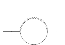
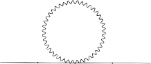
Figure 1: Correction to the scalar two point function from an intermediate scalar and graviton.

Figure 2: Correction to the scalar two point function from a graviton bubble.

The computation of these diagrams has always been performed in a pure de Sitter space [5, 6, 7, 8, 9, 10, 11, 12, 13]. However, some authors have also discussed the case of a quasi de Sitter background [11, 13]. In order to discuss the IR divergences, we will not need to know the whole expression for these diagrams. Those can be found, for example in Refs. [8, 9, 10, 11]. Furthermore, our observations are largely independent of de Sitter or quasi de Sitter. Let us briefly list here the main differences. In a pure de Sitter case the scalar metric perturbations are pure gauge, and the only physical perturbations are the tensor ones, i.e. that of the gravitons. In Eqs. (10, 11), $\nu$ becomes equal to ${3/2}$ in a pure de Sitter case.

In a quasi de Sitter case the de Sitter scale invariance is broken, which results in a modification of the term ${z^{\prime\prime}/z}$ in Eq. (10). It is evident from the experiments that the breaking is very small, within the observable ranges of scales relevant for the CMBR measurements, which corresponds to roughly $7$ e-foldings of inflation. It can be parametrized with the slow-roll parameter: $\epsilon=-{\dot{H}/H^{2}}\,.$ The solution to the field Eqs. (10, 11) now has $\nu={3/2}+{(1-n)/2},$ where $n$ is the spectral index . For a red-tilded spectrum, as the one observed for scalar perturbations, i.e. $n-1<0$, the IR divergences of the loop integrals become worse than that of the pure de Sitter case.

The computation of the diagrams is quite involved. Their structure is not immediately transparent for what concerns the physical interpretation of the IR divergences. In particular, the diagrams have two types of integrations - one over the (conformal) times for each of the vertices, and the other over the loop momentum. There are two possible sources of IR “divergences”. One comes from the time integrals and it is present only for some kind of interactions [7]. In our scenario it will not appear, while, in theories where it does, it is believed to be cured in realistic models by using the dynamical renormalization group techniques [10] (see also [7]). The other IR divergence comes from the momentum integral and it is always present. We will concentrate on this latter one.

We briefly discuss the issues regarding the regularization (“box approach”) of the IR divergent integrals. This analysis is actually important to understand that when the dependence on the cutoffs is not eliminated, the IR issue is not fully understood, although the corrections can be made sufficiently small. The important point here is that there is no unique choice for the IR cutoffs, rendering the results for the observable quantities ambiguous.

For instance, the main difference for the IR divergence in the momentum integration arises from the choice of imposing a cutoff on the physical or on the comoving momentum. To understand its consequences, we consider the example of a pure de Sitter case and the simplest IR divergent integral, that for example comes from Fig. 2:

$$\Lambda^{(\phi)}(\eta)={1\over(2\pi)^{3}}\int d^{3}kW_{k}(\eta,\eta)\,.$$ (14)

By choosing the cutoffs on the physical momentum, $p_{UV/IR}=M_{UV/IR}$, where $M_{UV/IR}$ does not depend on time, as in [10], one finds that for small $\eta$

$$\Lambda(\eta)\sim{1\over 2\pi^{2}}\int^{aM_{UV}}_{aM_{IR}}{dk\over k}H^{2}={H^{2}\over 2\pi^{2}}\log\left({M_{UV}\over M_{IR}}\right)\,.$$ (15)

The rationale behind this choice is that this kind of cutoffs does not break de Sitter scale invariance.

Instead, choosing the cutoffs on the comoving wavenumber as, $k_{UV/IR}=K_{UV/IR}$, where $K_{IR}$ is independent of time, as in Ref.  [11], and $K_{UV}=a(\eta)\mu$, where $\mu$ is the renormalization scale, one finds

$$\Lambda(\eta)\sim{1\over 2\pi^{2}}\int^{K_{UV}}_{K_{IR}}{dk\over k}H^{2}={H^{2}\over 2\pi^{2}}\log\left({K_{UV}\over K_{IR}}\right)\approx{H^{2}\over 2\pi^{2}}N_{\eta},$$ (16)

where $N_{\eta}$ is the number of efoldings from the beginning of inflation up to time $\eta$ and we have neglected the UV contribution proportional to $\log{\mu\over H}$. This kind of cutoffs does break de Sitter scale invariance. The rationale behind this choice is that we integrate over modes that were sub-Hubble at the beginning of inflation, $K_{IR}=a_{i}H_{i}$.

We see that Eqs. (15, 16) give very different results. First principles do not instruct us to prefer a cutoff either on the physical or the comoving momenta, and thus the scale dependence of the “observable” changes depending on the cutoff, which clearly makes it unphysical. The fact that the correlators grow with the IR cutoff, that is the “size of the box” $L=K_{IR}^{-1}$ also creates difficulty in approximating the ensemble averages via the spatial averages, which are performed in practical observations. In fact, the RMS deviation between the spatial and the ensemble averages goes like $\Delta P_{k}\sim{P_{k}/(kL)^{3/2}}$ [30], in the case of the spectrum, and, since $P_{k}$ grows with $L$ due to the IR divergences of the quantum loops, it could become non-negligible and should be taken into account for precise measurements and predictions, for not too large boxes and for certain scales (in particular for scales not too different from the “box size”). The solution to this problem is to apply the ergodic theorem only to the true IR-safe correlators.

To resolve the issue of IR divergences, we must then propose a recipe for the definition of a sensible perturbation theory that does not have any of the ambiguities we have presented.

4 Eliminating IR divergences

Our solution of the infrared issue will be centered on the concept of local observer, as we said in the introduction. In particular, our implementation of the principle of locality, will be different from the one dealt with, for example, in [22, 23], which consists in using gauge transformations that are singular at large scales. It will also differ, as we will see, from the approach in [20, 21], which, in particular, uses an explicit cutoff $q_{0}$, of the size of the typical scale of observations, when proposing how to resum the contributions from scales larger than $q_{0}^{-1}$ .

Our presentation is divided in three parts: in section 4.1 we investigate the physical point at the origin of the infrared divergences, by discussing what the true observables are and why the in-in formalism, as it stands now, does not properly account for them. In section 4.2 we demonstrate that all infrared divergences from momentum integrals in gravitational loops have a common origin, which is precisely the unphysical element of the formalism presented in section 4.1. Finally, in section 4.3 we outline our solution of the infrared issue proposing a more physical redefinition of the in-in formalism. A detailed example of how our proposal is implemented is given in section 4.4.

Our notation will be as follows: we will write the background FRW metric as $g_{\mu\nu}$:

$$ds^{2}=g_{\mu\nu}dx^{\mu}dx^{\nu}=-dt^{2}+a^{2}\delta_{ij}dx^{i}dx^{j}.$$ (17)

and, in our conventions, the background quantities, which are contracted using the background metric, have no labels: for example $k^{2}=\delta^{ij}k_{i}k_{j}$.

The perturbed quantities are instead indicated by ”over-bar”. Thus, the local classical metric is given by (neglecting the vector part):

$$\overline{ds}^{2}=\overline{g}_{\mu\nu}dx^{\mu}dx^{\nu}=-\overline{N}^{2}dt^{2}+a(t)^{2}\overline{h}_{ij}(dx^{i}+\overline{N}^{i}dt)(dx^{j}+\overline{N}^{j}dt)$$ (18)

where $N^{i},N$ are the shift and lapse functions, and 

$$\overline{h}_{ij}dx^{i}dx^{j}=e^{2\zeta(\vec{x},t)}(e^{\gamma(\vec{x},t)})_{ij}dx^{i}dx^{j}\,.$$ (19)

The quantities contracted with this metric will have an ”over-bar”, for example $\overline{k}^{2}=\overline{h}^{ij}k_{i}k_{j}$.

4.1 True observables and in-in formalism

We will here argue that the usual formalism for the perturbation theory does not define correctly the observables from the point of view of a local observer, and this is the origin of the IR divergences.

Let us look closely at the definition of observables in the in-in formalism. For definiteness, let us consider the two-point function as a working example (our considerations apply also to $N$-point functions, as we will discuss in section 4.5). The definition of the observables in the perturbative in-in formalism is given by the right-hand side of Eq. (13). The important element in this formula is that the observables are defined in terms of the background quantities, in particular the background metric (entering for example in $k^{2}$). However, the background metric has no physical meaning and we claim that this is the reason of an appearance of the IR divergences.

In fact, any local observer uses true local clocks and ruler. The observer has no notion of a “background metric” and “perturbations” on it, but instead he/she uses the local metric for his/her measurements. We will show that when writing the perturbative correlators from the point of view of the local observer, that is using the local metric, the IR divergences are cured.

In more details, the IR divergences arise for the following reason. In the in-in formalism, the perturbations ($\zeta,\gamma$) are promoted to quantum fields ($\widehat{\zeta},\widehat{\gamma}$), and path-integrated using the background metric of Eq. (17) to contract the indices. We will show that in the correlators at loop level, all IR divergences arise when at least one of the momenta running in the loops lines goes to zero. In that limit the correlator becomes effectively disconnected and leads to the IR divergences. We represent this, schematically, in Fig. 3.

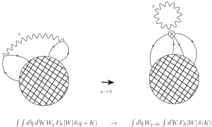
Figure 3: A schematic representation of the loop corrections in an IR limit as shown in the text. A generic correlator can be written, taking care of the time-ordering, as a product of Whigtman functions integrated over the momenta running in the internal lines, with delta functions at vertices. In the IR limit of a diagram line (for example, here in the picture, a graviton’s one), the total correlator factorizes into the product of a disconnected two-point function at small momentum times the rest of the correlator with a certain “vertex”. The disconnected two-point function (when $q\rightarrow 0$) leads to the IR divergences. We will show that when redefining the correlators using the local metric, the disconnected contributions disappear.

We claim that it is precisely these operations of expansion over the background metric and quantum averaging of the perturbations in effectively disconnected contributions that make no sense from the point of view of an observer. These are the unphysical elements of the standard in-in perturbation theory, because a local observer will not be sensitive to the background metric Eq. (17), but to the local metric Eq. (18), whose classical value in the quantum theory is

$$\overline{g}_{\mu\nu}=\langle\,\widehat{\overline{g}}_{\mu\nu}\,\rangle\,,$$ (20)

where, in particular,

$$\overline{h}_{ij}=\langle e^{2\widehat{\zeta}(\vec{x},t)}(e^{\widehat{\gamma}(\vec{x},t)})_{ij}\rangle\,.$$ (21)

We will show in section 4.3 that by correctly defining the correlators in terms of the local classical metric Eqs. (18), (21) these disconnected pieces will be removed and the infrared issue cured. Our IR-safe correlators will be different from those defined in other proposals, as for example in [20, 21] or [22, 23].

4.2 IR divergences at all order

We will now prove that indeed all IR divergences from momenta integrals originate in the unphysical expansion of the local metric in perturbations and their path integration in the IR limit where higher order correlators become disconnected, as we have claimed in the previous section. Here, we will focus on the two-point function for scalar perturbations, but our analysis can be extended to the general case of $N$-point functions and to gravitons.

Let us first review in some detail the path-integral formulation of the in-in perturbation theory, for a general reference see [6]. The Lagrangian we are keen to discuss is the one of a nearly massless scalar field, $\sigma$, which could be the inflaton, minimally coupled to gravity,

$$S={1\over 2}\int\sqrt{-\text{det}(\overline{g})}\left[\overline{R}-\overline{g}_{\mu\nu}\partial_{\mu}\sigma\partial_{\nu}\sigma-2V(\sigma)\right]\,,$$ (22)

where $V(\sigma)$ is very flat, otherwise arbitrary. Using the ADM formalism [31], the action becomes

$$S={1\over 2}\int\sqrt{-\text{det}(\overline{h})}~{}{a^{3}\over 2}~{}e^{3\zeta}\Bigg{[}\overline{N}\overline{R}^{(3)}-2\overline{N}V(\sigma)+\overline{N}^{-1}\Big{(}\overline{E}^{j}{}_{i}\overline{E}^{i}{}_{j}-(\overline{E}^{i}{}_{i})^{2}\Big{)}+\\ +\overline{N}^{-1}\Big{(}\dot{\sigma}-\overline{h}^{ij}\overline{N}_{i}\partial_{j}\sigma\Big{)}^{2}-\overline{N}a^{-2}e^{-2\zeta}[\exp{(-\gamma)}]^{ij}\partial_{i}\sigma\partial_{j}\sigma\Bigg{]}\;,$$ (23)

where

$$\overline{E}_{ij}\equiv\frac{1}{2}\Big{(}\dot{\overline{h}}_{ij}-\nabla_{i}\overline{N}_{j}-\nabla_{j}\overline{N}_{i}\Big{)}\;;$$ (24)

$\nabla_{i}$ is the three-dimensional covariant derivative calculated with the three-metric $\overline{h}_{ij}$; and $\overline{R}^{(3)}$ is the curvature scalar calculated with this three-metric:

$$\overline{R}^{(3)}=a^{-2}e^{-2\zeta}\Big{[}e^{-\gamma}\Big{]}^{ij}~{}\overline{R}^{(3)}_{ij}.$$

All spatial indices $i$, $j$, etc. are lowered and raised with the metric $\overline{h}_{ij}$ and its reciprocal. In particular, by computing the derivatives, such as $\dot{\overline{h}}_{ij}$ in Eq. (24), one can find a kinetic term for $\zeta$ and $\gamma$, where indices are contracted by $\overline{h}_{ij}$. We choose the gauge where the scalar field is homogeneous, and $\zeta\neq 0$.

The two-point function in the standard in-in perturbation theory (using the path-integral formulation) is obtained by expanding the metric $\overline{h}_{ij}$ in terms of the perturbations $\zeta,\gamma$. In this section we will not indicate quantum fields with $\;\widehat{\mbox{}}\;$ in order not to clutter the equations. The formalism also requires doubling the field degrees of freedom in order to account for the time ordering and anti-ordering in Eq. (12): $\zeta\to\{\zeta_{+},\zeta_{-}\}$, and similarly for $\gamma$. It will appear to be convenient to change basis to $\zeta_{C}={1\over 2}(\zeta_{+}+\zeta_{-})$, $\zeta_{\Delta}=\zeta_{+}-\zeta_{-}$, and the analogous for the $\gamma$.

The perturbative expansion in terms of the perturbations $\zeta,\gamma$ is obtained by functionally Taylor-expand the exponential $e^{i\int_{\eta_{\text{in}}}^{\eta}d\tau\int d^{3}x\sqrt{-det\,\overline{h}}\,\mathcal{L}(\zeta_{C},\gamma_{C},\zeta_{\Delta},\gamma_{\Delta})}$ in the path integral in powers of the perturbations $\zeta_{C},\gamma_{C},\zeta_{\Delta},\gamma_{\Delta}$:

$$\int{d^{3}k_{1}\over(2\pi)^{3}} \int{d^{3}k_{1}\over(2\pi)^{3}}e^{i\vec{k}_{1}\cdot\vec{x}_{1}+i\vec{k}_{2}\cdot\vec{x}_{2}}\langle\zeta(x_{1},\eta)\zeta(x_{2},\eta)\rangle=$$

$$\int{d^{3}k_{1}\over(2\pi)^{3}}\int{d^{3}k_{1}\over(2\pi)^{3}}e^{i\vec{k}_{1}\cdot\vec{x}_{1}+i\vec{k}_{2}\cdot\vec{x}_{2}}\int_{\mathcal{C}}\mathcal{D}\zeta_{C}\mathcal{D}\zeta_{\Delta}\mathcal{D}\gamma_{C}\mathcal{D}\gamma_{\Delta}\,\zeta_{C}(x_{1},\eta)\zeta_{C}(x_{2},\eta)\,$$

$$\sum_{\begin{subarray}{c}n,m,\\ u,v\geq 0\end{subarray}}{1\over n!m!u!v!}\prod_{a=0}^{n}\biggl{(}\int d^{3}x_{(a)}d\eta_{(a)}\zeta_{C}\text{{\small$(\vec{x}_{(a)},\eta_{(a)})$}}{\delta\over\delta\zeta_{C}\text{{\small$(\vec{x}_{(a)},\eta_{(a)})$}}}\biggr{)}$$

$$\qquad\prod_{b=0}^{m}\biggl{(}\int d^{3}x_{(b)}d\eta_{(b)}\gamma_{\text{{\tiny$Ci_{(b)}j_{(b)}$}}}\text{{\small$(\vec{x}_{(b)},\eta_{(b)})$}}{\delta\over\delta\gamma_{\text{{\tiny$Ci_{(b)}j_{(b)}$}}}\text{{\small$(\vec{x}_{(b)},\eta_{(b)})$}}}\biggr{)}$$

$$\qquad\prod_{c=0}^{u}\biggl{(}\int d^{3}x_{(c)}d\eta_{(c)}\zeta_{\Delta}\text{{\small$(\vec{x}_{(c)},\eta_{(c)})$}}{\delta\over\delta\zeta_{\Delta}\text{{\small$(\vec{x}_{(c)},\eta_{(c)})$}}}\biggr{)}$$

$$\qquad\prod_{d=0}^{v}\biggl{(}\int d^{3}x_{(d)}d\eta_{(d)}\gamma_{\text{{\tiny$\Delta\,i_{(d)}j_{(d)}$}}}\text{{\small$(\vec{x}_{(d)},\eta_{(d)})$}}{\delta\over\delta\gamma_{\text{{\tiny$\Delta\,i_{(d)}j_{(d)}$}}}\text{{\small$(\vec{x}_{(d)},\eta_{(d)})$}}}\biggr{)}$$

$$\quad\qquad\;\;e^{i\int_{\eta_{\text{in}}}^{\eta}d\tau\int d^{3}x\sqrt{-det\,\overline{h}}\,\mathcal{L}(\zeta_{C},\gamma_{C},\zeta_{\Delta},\gamma_{\Delta},\overline{h}_{C},\overline{h}_{\Delta})}\Psi_{\text{vac},C}(\eta_{\text{in}})\Psi_{\text{vac},\Delta}(\eta_{\text{in}})\,,$$ (25)

where $\mathcal{C}$ is the closed time path, defined by $\zeta_{+}(\eta_{\text{in}})=\zeta_{-}(\eta_{\text{in}})$ (similarly for other fields), and the vacuum function is $\Psi_{\text{vac},C/\Delta}$. Finally, $\mathcal{L}(\zeta_{C},\gamma_{C},\zeta_{\Delta},\gamma_{\Delta},\overline{h}_{C},\overline{h}_{\Delta})=\mathcal{L}(\zeta_{+},\gamma_{+},\overline{h}_{+})-\mathcal{L}(\zeta_{-},\gamma_{-},\overline{h}_{-}),$ and, after the functional derivations, $\zeta_{C},\gamma_{C},\zeta_{\Delta},\gamma_{\Delta}\to 0$, $\overline{h}_{ij}\to\delta_{ij}$, in $\mathcal{L}$ for the usual Taylor expansion around the unperturbed background.

We are now ready to investigate what kind of IR divergences from momentum integrals are present in the cosmological perturbation theory in a (quasi) de Sitter background.

We find that all these IR divergences, at all orders, appear when a momenta running in a loop line goes to zero, as we claimed. The proof of this is as follows: in the perturbation theory over (quasi) de Sitter, the Whightman functions go as :

$$\sim{1\over|\vec{p}|^{3}}={1\over|\vec{k}-\vec{q}|^{3}}={1\over(|\vec{k}|^{2}+|\vec{q}|^{2}-2|\vec{k}||\vec{q}|\cos{\theta})^{3\over 2}}\,,$$ (26)

and therefore this would diverge only when $\vec{p}=0$. This happens when the momentum running in the line goes to zero.

In particular, there are no collinear divergences arising when two momenta are parallel, because the denominator of the Whightman functions (from which all other propagators can be obtained) never goes to zero in that case. This is very different from what happens in a scattering amplitude on Minkowski background, where such collinear divergences are present, for example when a soft gluon (or graviton) line originates from a massless line yielding a contribution to the diagram of the form: $\sim{1\over p^{\mu}p_{\mu}}={1\over(k-q)^{\mu}(k-q)_{\mu}}={1\over-2k^{\mu}q_{\mu}}$, which diverges when $k^{\mu}$ is parallel to $q^{\mu}$.

The IR divergences in momentum loops in perturbation theory can therefore all be recovered by taking the small momentum limit of the propagators in the relevant loop lines. Now we want to prove the other claim of ours: that all the IR divergences appear from disconnected contributions to the correlators. The relevant propagators in the usual $\pm$ basis are:

$$G^{-+}(\eta,\eta^{\prime}) =W(\vec{x},\eta,\vec{x}^{\prime},\eta^{\prime})\,,\qquad G^{+-}(\eta,\eta^{\prime})=W(\vec{x},\eta^{\prime},\vec{x}^{\prime},\eta)\,,$$

$$G^{++}(x,y) =\theta(\eta-\eta^{\prime})G^{-+}(\eta,\eta^{\prime})+\theta(\eta^{\prime}-\eta)G^{+-}(\eta,\eta^{\prime})\,,$$ (27)

$$G^{--}(x,y) =\theta(\eta-\eta^{\prime})G^{+-}(\eta,\eta^{\prime})+\theta(\eta^{\prime}-\eta)G^{-+}(\eta,\eta^{\prime})\,,$$

where $W(\vec{x},\eta,\vec{x}^{\prime},\eta^{\prime})$ is the Whightman function (recall Eq. (7)). Note that $G^{++}+G^{--}=G^{+-}+G^{-+}$. In the new, more convenient, ($C,\Delta$) basis the correlation functions are

$$\left(\begin{array}[]{cc}G_{C}&G_{R}\\ G_{A}&0\\ \end{array}\right)=Q\left(\begin{array}[]{cc}G^{++}&G^{+-}\\ G^{-+}&G^{--}\\ \end{array}\right)Q^{T}\,,\qquad Q=\left(\begin{array}[]{rrr}{1\over 2}&&{1\over 2}\\ 1&&-1\\ \end{array}\right)\,.$$ (28)

The advanced and retarded propagators are related by $G_{A}(x,y)=G_{R}(y,x)$ and vanish in the coincidence limit. The convenience in using this basis descends from the fact that in the IR limit (small momentum), the propagators behave as follows

$$G_{C}(q\equiv|\vec{q}|,\eta,\eta^{\prime})\underset{q\to 0}{\simeq}W(q,\eta,\eta^{\prime})|_{q\to 0}\sim{H^{2}\over q^{(4-n)}}\,,\qquad G_{R}(q,\eta,\eta^{\prime})\underset{q\to 0}{\sim}\theta(\eta-\eta^{\prime}){(\eta^{2\nu}-\eta^{{}^{\prime}\,2\nu})\over(\eta\eta)^{{}^{\prime}\,{{3\over 2}-\nu}}}$$ (29)

and therefore the IR divergences coming from the vanishing of the momentum in loop lines are accounted for by the $G_{C}$ propagator only. We concentrate therefore on the expansion in $\zeta_{C},\gamma_{C}$.

Let us then see how all these IR divergences arise from disconnected contributions to the correlators. It is easy to do it now that we have shown that they all arise when one (or more) momenta in a diagram line goes to zero. Indeed, the small momentum limit of the propagators can be found using the expansion of the perturbation fields given by Eq. (5), where - we recall - we have chosen planar coordinates: $Y_{\vec{k}}(\vec{x})=e^{i\vec{k}\cdot\vec{x}}$. In this limit, $Y_{\vec{k}}(\vec{x})\sim 1$, and thus the momenta of the lines sent to this IR limit drop out of the delta functions at the interaction vertices in Eq. (4.2). Therefore, in the IR limit the contributions of these lines to the two-point function become disconnected, and Eq. (4.2) reads, once written in momentum space, as:

$$\!\!\!\!\langle\zeta(k_{1},\eta)\zeta(k_{2},\eta)\rangle_{\text{IR, all orders}}\!\!=\!\!\sum_{n,m\neq(0,0)}{1\over n!m!}\!\!\prod_{\begin{subarray}{c}0\leq a\leq n\\ 0\leq b\leq m\end{subarray}}\biggl{(}\!\int d\eta_{(a)}d\eta_{(b)}\!\biggr{)}\langle\prod_{a=0}^{n}\zeta_{C}(\eta_{(a)})\rangle_{{}_{\text{(IR)}}}\langle\prod_{b=0}^{m}\gamma_{C\,i_{(b)}j_{(b)}}(\eta_{(b)})\rangle_{{}_{\text{(IR)}}}\\ \int_{\mathcal{C}}\mathcal{D}\zeta_{C}\mathcal{D}\zeta_{\Delta}\mathcal{D}\gamma_{C}\mathcal{D}\gamma_{\Delta}\,\zeta_{C}(k_{1},\eta)\zeta_{C}(k_{2},\eta)\,\prod_{a=0}^{n}\biggl{(}\int d^{3}x_{(a)}{\delta\over\delta\zeta_{C}(\vec{x}_{(a)},\eta_{(a)})}\biggr{)}\\ \prod_{b=0}^{m}\biggl{(}\int d^{3}x_{(b)}{\delta\over\delta\gamma_{Ci_{(b)}j_{(b)}}(\vec{x}_{(b)},\eta_{(b)})}\biggr{)}\,\,e^{i\int_{\eta_{\text{in}}}^{\eta}d\tau\int d^{3}x\sqrt{-\text{det}\overline{h}}\,\mathcal{L}(\zeta_{C},\gamma_{C},\zeta_{\Delta},\gamma_{\Delta},\overline{h}_{C},\overline{h}_{\Delta})}\Psi_{\text{vac},C}(\eta_{\text{in}})\Psi_{\text{vac},\Delta}(\eta_{\text{in}})\,,$$ (30)

where again, having Taylor expanded, $\zeta_{C},\gamma_{C},\zeta_{\Delta},\gamma_{\Delta}\to 0$, $\overline{h}_{ij}\to\delta_{ij}$, in $\mathcal{L}$ after the functional derivations. The label ${}_{{}_{\text{(IR)}}}$ indicates the small momentum limit of the propagators (infrared divergent).

We have thus proven that the equation (30) comprises all the IR-divergent parts of the two-point correlator from loop momenta integrations, and these appear as disconnected contributions. With a more schematic and shortcut notation, we can write Eq. (30) as

$$\langle\zeta(k_{1},\eta)\zeta(k_{2},\eta)\rangle_{\text{IR, all orders}}=\\ \sum_{n,m\neq(0,0)}{1\over n!m!}\,\langle\prod_{u=0}^{n}\zeta\rangle_{\text{{\tiny IR}}}\,\langle\prod_{v=0}^{m}\gamma_{i_{(v)}j_{(v)}}\rangle_{\text{{\tiny IR}}}\,{\partial^{n}\over\partial\zeta_{{}_{\bar{h}}}^{n}}\,{\partial^{m}\over\partial\gamma_{{}_{\bar{h}}i_{(v)}j_{(v)}}^{m}}\,\,\langle\zeta(k_{1},\eta)\zeta(k_{2},\eta)\rangle\,.$$ (31)

With the suffix $\mbox{}_{{}_{\bar{h}}}$ we indicate that the derivatives do not act on the external fields, $\zeta(k_{1},\eta),\zeta(k_{2},\eta)$, of the correlator, but on the fields entering the correlator via its dependence on $\overline{h}_{ij}=e^{2\zeta}(e^{\widehat{\gamma}})_{ij}$.

The form of Eq. (31) makes it even more evident that the IR divergences are a result of the expansion of the local perturbed metric over the long-wavelength perturbations and the path integration in the limit where higher order correlators become disconnected. This result completes and extends that in Ref.  [11], where it was shown that some IR divergences in certain one-loop in-in computations could be recovered from semiclassical expansions around the perturbed metric . We have here proven, using a rigorous field theory formalism, that all the IR divergences in momentum integrals in gravitational loops at all orders are accounted for by the equation (31). The demonstration applies to $N$-point function for all $N$’s as well.

Since now we see that all IR divergences in gravitational loops have the same origin, whose nature we can understand, we will propose a procedure to fully resolve them on the basis of the physical concepts discussed in section 4.1. In the next section we turn to this point.

4.3 Defining a different in-in perturbation theory

We set out now to define a new perturbative expansion in the in-in formalism, capable of curing the infrared issue. We will outline our recipe, and comment on how it differs from other proposals concerning the IR issue. For definiteness, we will be illustrating our proposal on the two-point correlator $\langle\zeta(k_{1},\eta)\zeta(k_{2},\eta)\rangle$, but, just as before, our considerations also apply to $\langle\gamma\gamma\rangle$, or any other correlator of $N$ fields, for all $N$’s.

In the usual perturbation theory around the background metric, the two-point correlator is given by a series

$$\langle\zeta(k_{1},\eta)\zeta(k_{2},\eta)\rangle=\mathcal{A}(k,\eta)\delta(\vec{k}_{1}+\vec{k}_{2})=\bigl{(}\mathcal{A}(k,\eta)_{{}_{\text{tree}}}+\mathcal{A}(k,\eta)_{{}_{\text{loops}}}\bigr{)}\delta(\vec{k}_{1}+\vec{k}_{2})$$ (32)

We stress that we do not take any infrared limit of sorts here, but instead we are considering the full perturbative series ($\mathcal{A}(k,\eta)_{{}_{\text{loops}}}=\mathcal{A}(k,\eta)_{{}_{\text{1-loop}}}+\mathcal{A}(k,\eta)_{{}_{\text{2-loop}}}+\ldots$) with the loops contributions including the ultraviolet, finite and infrared parts altogether (as we are not concerned here with the ultraviolet divergences, we will assume that all correlators here and in the following are suitably renormalized).

The background metric enters in this formula because it is used to contract the comoving momenta as (recall that we use the ADM formalism)

$$k^{2}=h_{{}_{\text{bckgr}}}^{ij}\,k_{j}k_{j}=\delta^{ij}\,k_{j}k_{j}$$ (33)

where we have used $h_{{}_{\text{bckgr}}}^{ij}=\delta^{ij}$.

Motivated by our results and understanding in the previous sections, we set out to define a new perturbation theory, where scales are not defined by contracting with the background metric, but with the field

$$\overline{h}_{ij}=\langle e^{2\widehat{\zeta}(\vec{x},t)}(e^{\widehat{\gamma}(\vec{x},t)})_{ij}\rangle\,.$$ (34)

The idea, let us repeat it once again, is that in this way we should be able to take into account the actual local metric that defines scales for the observer. We want to see if in this way the infrared issue will be cured or not. Please, observe that in this definition, the notation $\langle~{}~{}\rangle$ indicates a quantum expectation value in the in-vacuum and that $\widehat{\zeta},\,\widehat{\gamma}$ are the full quantum fields. Therefore the definition of $\overline{h}$ is the standard definition of the classical field as the in-vacuum quantum average of a quantum operator. In particular, it is not based on any infrared limit or large scale averaging or any infrared/large scale definition/quantity/procedure.

As the background metric was entering the correlators by contracting the wavenumbers $k$, the new field $\overline{h}$ (the local metric) will have to be used to contract the wavenumbers in place of the background metric, as

$$\overline{k}^{2}=(\overline{h})^{ij}\,k_{j}k_{j}=\langle e^{-2\widehat{\zeta}(\vec{x},t)}(e^{-\widehat{\gamma}(\vec{x},t)})^{ij}\rangle\;k_{i}k_{j}.$$ (35)

Note that this quantity is very different from the one defined in Refs [20, 21], which is

$$\kappa(q_{0},L)^{2}=e^{-2\zeta_{ir}(\vec{x},t)}(e^{-\gamma_{ir}(\vec{x},t)})_{ij}k^{i}k^{j}\,;$$ (36)

the latter quantity is in fact defined by using the large scale behavior

$$\zeta_{ir}/\gamma_{ir}=(2\pi)^{-{3\over 2}}\underset{L^{-1}<q\ll q_{0}}{\int}d^{3}qe^{i\vec{k}\cdot\vec{x}}\zeta_{\vec{k}}/\gamma_{\vec{k}}\;,$$ (37)

where $q_{0}$ is a suitable cutoff defining an infrared/large scale limit where the fields become classical. As we said, we use instead the full quantum fields and the usual quantum vacuum expectation value, see equation (34). The logic at the basis of the proposal in Refs [20, 21] and of equation (36) is the definition of a different background, characterized by the scale $q_{0}$, taking into account superhorizon modes, on which to do a new perturbation theory. Their power spectrum is defined as the Fourier transform of a spatial average at two points $\vec{x}_{1}$ and $\vec{x}_{2}=\vec{x}_{1}+\vec{y}$ with $q_{0}^{-1}\sim y$ and then distances are rescaled with the new background metric, which is not fully local as well (it depends on $q_{0}^{-1}\sim|\vec{x}_{2}-\vec{x}_{1}|$).

We, instead, put the physical concept of locality at the basis of our redefinition of the perturbation theory, asking what a local observer would actually use: (34) is not a background metric, but the local metric that the observer would use to define scales and a local quantities. Further differences among the other proposals and ours will soon appear.

At first sight, at this point we can construct two kind of correlators using $\overline{h}$ that we might think to use to define a new perturbation theory:

$$\mathcal{A}^{\prime}(\overline{k},\eta)=\mathcal{A}^{\prime}(\overline{k},\eta)_{{}_{\text{tree-level}}}+\mathcal{A}^{\prime}(\overline{k},\eta)_{{}_{\text{loops}}}\,,$$ (38)

or

$$\mathcal{A}(\overline{k},\eta)=\mathcal{A}(\overline{k},\eta)_{{}_{\text{tree-level}}}+\mathcal{A}(\overline{k},\eta)_{{}_{\text{loops}}}\,.$$ (39)

Here, the first object $\mathcal{A}^{\prime}(\overline{k},\eta)$ is the transformed two-point correlator under the transformation $k\to\overline{k}$ acting as a change of coordinates. The second object $\mathcal{A}(\overline{k},\eta)$ is instead the non-transformed correlator evaluated on the newly contracted $\overline{k}$. We claim that the latter is the one we should use for the new perturbation theory.

In fact, it is straightforward to see that (38) does not give any new perturbation theory, because $\mathcal{A}^{\prime}(\overline{k},\eta)=\mathcal{A}(k,\eta)$, since the correlators transform as scalar under the transformation $k\to\overline{k}$, and thus we would be just re-writing in new coordinates the same old perturbation theory, with all the same problems.

Instead $\mathcal{A}(\overline{k},\eta)$ is obviously different from $\mathcal{A}(k,\eta)$ and thus defines a new perturbation theory. It is straightforward to obtain the explicit expression of $\mathcal{A}(\overline{k},\eta)$ in terms of $\mathcal{A}(k,\eta)$, by using standard techniques in calculus and the action of diffeomorphisms. We briefly illustrate the passages:

• we take the correlator $\mathcal{A}(k,\eta)$ (which comprises the tree-level and all loop contributions, see equation (32)) and transform its $k$-dependence into a $k(\overline{k})$-dependence using

  $$k^{2}=(\overline{h}^{-1})^{ij}\,\overline{k}_{j}\overline{k}_{j}=\langle e^{2\widehat{\zeta}(\vec{x},t)}(e^{\widehat{\gamma}(\vec{x},t)})^{ij}\rangle\;\overline{k}_{i}\overline{k}_{j},$$ (40)

• we then expand in Taylor series:

  $$\mathcal{A}(k(\overline{k}),\eta)=\mathcal{A}(\overline{k},\eta)\big{|}_{\zeta_{{}_{\bar{h}}}=\gamma_{{}_{\bar{h}}}=0}+\!\!\!\!\sum_{\begin{subarray}{c}n,m\geq 0\\ \{n,m\}\neq\{0,0\}\end{subarray}}{1\over n!m!}\langle(\widehat{\zeta})^{n}\rangle\langle(\widehat{\gamma}^{ij})^{m}\rangle\partial_{\zeta_{{}_{\bar{h}}}}^{n}\partial_{\gamma^{ij}_{{}_{\bar{h}}}}^{m}\mathcal{A}(k,\eta)\big{|}_{\begin{subarray}{c}\zeta_{{}_{\bar{h}}}=\gamma_{{}_{\bar{h}}}=0\\ (k^{2}=\overline{k}^{2})\end{subarray}}\,,$$ (41)

• we finally note that the first term on the right hand side of Eq. (41), i.e.

  $$\mathcal{A}(\overline{k},\eta)\big{|}_{\zeta_{{}_{\bar{h}}}=\gamma_{{}_{\bar{h}}}=0} =\mathcal{A}(k(\overline{k}),\eta)-\!\!\!\!\sum_{\begin{subarray}{c}n,m\geq 0\\ \{n,m\}\neq\{0,0\}\end{subarray}}{1\over n!m!}\langle(\widehat{\zeta})^{n}\rangle\langle(\widehat{\gamma}^{ij})^{m}\rangle\partial_{\zeta_{{}_{\bar{h}}}}^{n}\partial_{\gamma^{ij}_{{}_{\bar{h}}}}^{m}\mathcal{A}(k,\eta)\big{|}_{\begin{subarray}{c}\zeta_{{}_{\bar{h}}}=\gamma_{{}_{\bar{h}}}=0\\ (k^{2}=\overline{k}^{2})\end{subarray}}\,$$ (42)

  is precisely the non-transformed correlator evaluated on $\overline{k}$, which we were looking for. Once again, we stress that we have not taken any infrared limit or similar, and that all higher order contribution include all ultraviolet, finite and infrared parts.

In fact, at this point it is not yet clear that the infrared issue has been cured in this way. In order to understand that, we need to look more carefully at the loops contribution in $\mathcal{A}(\overline{k},\eta)$ to assess better how the new formalism, centered around $\overline{h}$, differs from the old one centered around the background metric. Thus, by substituting (32), (38) in equation (42), we find that 

$$\mathcal{A}(\overline{k},\eta)_{{}_{\text{loops}}}=\mathcal{A}^{\prime}(\overline{k},\eta)_{{}_{\text{loops}}}-\sum_{\begin{subarray}{c}n,m\geq 0\\ \{n,m\}\neq\{0,0\}\end{subarray}}{1\over n!m!}\langle(\widehat{\zeta})^{n}\rangle\langle(\widehat{\gamma}^{ij})^{m}\rangle\partial_{\zeta_{{}_{\bar{h}}}}^{n}\partial_{\gamma^{ij}_{{}_{\bar{h}}}}^{m}\mathcal{A}(k,\eta)\big{|}_{\begin{subarray}{c}\zeta_{{}_{\bar{h}}}=\gamma_{{}_{\bar{h}}}=0\\ (k^{2}=\overline{k}^{2})\end{subarray}}\,.$$ (43)

Clearly, $\mathcal{A}(\overline{k},\eta)_{{}_{\text{loops}}}$ is different from zero, because the first term on the right hand side is not equal to the the second term (the sum over disconnected contributions), and thus their difference is not null. In fact the first term is the standard loops contribution, not given by disconnected diagrams. Recall that all terms at each order include their ultraviolet, finite and infrared parts altogether.

However, because of our results in section 4.2, we see that the infrared divergent parts do cancel between the first and the second term on the right hand side of equation (43) and thus $\mathcal{A}(\overline{k},\eta)$ is free of infrared divergences: looking at equation (31) it is straightforward to see that infrared divergences/Log-enhancements, and only those, do cancel out exactly order by order.

We stress that, instead, the ultraviolet (renormalized) and finite terms do not cancel between the first and second term and so the loop contributions $\mathcal{A}(\overline{k},\eta)_{{}_{\text{loops}}}$ in the new perturbation theory around $\overline{h}$ are 1) different from those in the standard perturbation theory using the background metric (thus the new perturbation theory is a non-trivial modification and in principle testable), and 2) have the bonus that the IR divergences are absent (without using any IR cutoff procedure to define the new theory).

As a comment, let us observe that, being fully expressed as a combination of usual standard coordinate-transformed correlators, as visible in equation (42), also the new correlators will be sharing the same properties of the old ones (such as conservation and alike) at large scales (large $\overline{k}$). Furthemore, since the field $\zeta$ is fully gauge invariant and, at the level of field equations, (35) acts as a coordinate transformation, $\zeta$ will be conserved on superhorizon $\overline{k}$-scales. Note also that we could have obtained our result using different gauge-fixed quantities (such as the inflaton perturbation) or even gauge-invariant variables such as the Bardeen potentials – in all cases the physical interpretation of the IR-divergences linked to the metric/clocks of the local observer is the same (a local dressing and rescaling of the metric or Hubble rate, see section 4) and the prescription for the IR-safe correlator, Eq. (42), changes only in the fact that the chosen perturbation variables must be used in place of $\zeta,\gamma$. Note that the action is indeed gauge independent, and therefore the vertices are well-defined.

As a final comment, it can be useful to compare our proposal with the one in Refs [20, 21]. As we have already shown that their proposal is based on a quantity $\kappa(q_{0},L)^{2}=e^{-2\zeta_{ir}}(e^{-\gamma_{ir}})_{ij}k^{i}k^{j}$, see Eq. (36), defined using $q_{0},L$ to define the classical fields $\zeta_{ir},\gamma_{ir}$ via the IR or large scale limit given by Eq. (37). We do not use any large scale limit in our case, but employ the quantum expectation value of the full quantum fields in our Eqs. (34), (35).

Moreover, the IR-safe two-point correlator  is also defined in a different way than in our case. Refs. [20, 21] define it via a transformation $k\to\kappa(q_{à},L)$ of the Fourier Transform of a spatial average at pair of points:

$$\mathcal{A}^{\prime}(\kappa(q_{0},L),\eta)_{\text{tree}}.$$ (45)

In other words, their proposal is to fix a certain physical cutoff $q_{0}$ corresponding to the typical scale of the observation ( $q_{0}^{-1}\sim|\vec{x}_{2}-\vec{x}_{1}|$, with $\vec{x}_{2},\vec{x}_{1}$ the pair of points of the average), and define as “infrared” all wave numbers $k<q_{0}$, essentially decomposing the fields as $\zeta=\zeta_{ir}^{k<q_{0}}+\zeta^{k>q_{0}}$, promoting only $\zeta^{k>q_{0}}$ to quantum fields (analogously is done for $\gamma$) and declaring the infrared safe correlators to be just the tree-level result written in the new variables, see Eq. (36).

The first question that arises here is: since the correlator in Eq. (45) is only the tree-level contribution, supplemented with the IR effects in Eq. (36), what would be the IR-safe loop corrections to it in the proposal of [20, 21]? The paper does not explicitly discuss this issue. It is however clear that because of the decomposition $\zeta=\zeta_{ir}^{k<q_{0}}+\zeta^{k>q_{0}}$, the loop corrections would have the form

$$\mathcal{A}^{\prime}(\kappa,\eta)_{\text{loop, with IR cutoff $q_{0}$}}.$$ (46)

and thus the total correlator is:

$$\mathcal{A}^{\prime}(\kappa,\eta)_{\text{tree}}+\mathcal{A}^{\prime}(\kappa,\eta)_{\text{loop, with IR cutoff $q_{0}$}}.$$ (47)

It is straightforward to see then, that, although the “IR-fields” are resummed in $\kappa$, equation (36) is indeed just given by a coordinate transformation , and the final outcome amounts in effect just to the use of an infrared cutoff $q_{0}$ in the loops. That is, there is in effect no difference with the usual “box cutoff” approach, with all the issues that we have discussed before.

It follows that there are big differences with our current proposal: we do not introduce any infrared cutoff whatsoever, not even an “observational” one like $q_{0}$, nor we decompose the fields as $\zeta=\zeta_{ir}^{k<q_{0}}+\zeta^{k>q_{0}}$. What we do is really to define a new perturbation theory on the basis of the quantum expectation value $\overline{h}=\langle e^{2\widehat{\zeta}}e^{\widehat{\gamma}}\rangle$ of the full quantum operator to define scales, instead than the standard perturbation theory around the background metric. The new perturbative correlators are given by the series Eq. (42), and the higher order corrections to correlators are non-trivial and do not reduce to the use of a cutoff in the old perturbation theory. It is straightforward to generalize to all $N$-point functions for both $\zeta$ and $\gamma$.

4.4 Example at one-loop

We now give a detailed example at one-loop that our procedure do cancel all IR divergences (Log-cutoff enhancements) while redefining the perturbative series, in the theory with the Lagrangian in (22). To keep the example simple, let us consider a pure de Sitter case, so that $\zeta=0,\sigma=\sigma(\vec{x},t)$. In this case, the only physical metric perturbations are gravitons. We wish to compute the IR-safe two-point correlator $\langle\sigma(\overline{k},\eta)\sigma(\overline{k}^{\prime},\eta)\rangle$, at one loop, following our recipe culminating in equations (42).

We start by computing the one-loop correlator using the standard in-in perturbation theory. We recall here the known results from Ref. [11]. The one-loop in-in loop corrections are given by the diagrams in Figs. 2 and 2. The relevant interaction Lagrangians are obtained by expanding the full Lagrangian in perturbation up to second order, and they read

$${\cal L}_{3}={a\over 2}\gamma^{ij}\partial_{i}\sigma\partial_{j}\sigma\ ,$$ (48)

$${\cal L}_{4}=-{a\over 4}\gamma^{il}\gamma_{l}^{\;j}\partial_{i}\sigma\partial_{j}\sigma\,,$$ (49)

where $a$ is scale factor of the de Sitter background. The computation is performed by using Eq. (12), and the details are quite complicated and of little interest here. We will give some of the intermediate steps, details can be found in Refs. [9, 11]. From the diagram in Fig. 2, we obtain two contributions

$$A_{k}(\eta) =-8{\rm Re}\int{d^{3}q\over(2\pi)^{3}}\int_{-\infty}^{\eta}{d\eta_{1}\over(H\eta_{1})^{2}}\int_{-\infty}^{\eta_{1}}{d\eta_{2}\over(H\eta_{2})^{2}}\omega_{ij,kl}(\vec{q})k^{i}k^{j}k^{k}k^{l}W_{q}(\eta_{1},\eta_{2})W_{k-q}(\eta_{1},\eta_{2})$$

$$\qquad\qquad\qquad\qquad\qquad\qquad\qquad\qquad\qquad\qquad\times W_{k}(\eta,\eta_{1})W_{k}(\eta,\eta_{2})$$ (50)

$$B_{k}(\eta) =4{\rm Re}\int{d^{3}q\over(2\pi)^{3}}\int_{-\infty}^{\eta}\prod_{i=1}^{2}{d\eta_{i}\over(H\eta_{i})^{2}}\omega_{ij,kl}(\vec{q})k^{i}k^{j}k^{k}k^{l}W_{q}(\eta_{1},\eta_{2})W_{k-q}(\eta_{1},\eta_{2})W_{k}(\eta_{1},\eta)W_{k}(\eta,\eta_{2}),$$ (51)

where $W_{a}(\eta,\eta^{\prime})$ is given by Eq. (8). From Fig. 2, we obtain

$$C_{k}(\eta)={\rm Re}\left[(-2i)\int{d^{3}q\over(2\pi)^{3}}\int\frac{d\eta^{\prime}}{(H\eta^{\prime})^{2}}\omega^{\phantom{i}l}_{i\phantom{l},lj}k^{i}k^{j}W_{q}(\eta^{\prime},\eta^{\prime}),W_{k}(\eta,\eta^{\prime})^{2}\right]\ .$$ (52)

The definition of the sum over graviton polarizations $\omega_{ij,kl}$ is

$$\omega_{ij,kl}(\vec{q}) =\sum_{s}\epsilon^{s}_{ij}(\vec{q})\epsilon^{s*}_{kl}(\vec{q}) =\delta_{ik}\delta_{jl}+\delta_{il}\delta_{jk}-\delta_{ij}\delta_{kl}$$ (53)

$$~{}~{}+\delta_{ij}\vec{\hat{q}}_{k}\vec{\hat{q}}_{l}+\delta_{kl}\vec{\hat{q}}_{i}\vec{\hat{q}}_{j}-\delta_{ik}\vec{\hat{q}}_{j}\vec{\hat{q}}_{l}-\delta_{il}\vec{\hat{q}}_{j}\vec{\hat{q}}_{k}-\delta_{jk}\vec{\hat{q}}_{i}\vec{\hat{q}}_{l}-\delta_{jl}\vec{\hat{q}}_{i}\vec{\hat{q}}_{k}+\vec{\hat{q}}_{i}\vec{\hat{q}}_{j}\vec{\hat{q}}_{k}\vec{\hat{q}}_{l}$$

where $\vec{\hat{q}}$ is the unit vector in the direction $\vec{q}$, and $\epsilon_{ij}$ is the graviton polarization tensor. After evaluating the integrals and regularizing it with IR and ultraviolet cutoffs, we get

$$\langle\sigma(k,\eta)\sigma(k^{\prime},\eta)\rangle_{\text{one-loop}} =A_{k}(\eta)+B_{k}(\eta)+C_{k}(\eta)$$

$$={2\over 15}\log(\Lambda_{IR}){H^{4}\over M_{\text{P}}^{4}}{1\over(2\pi)^{2}k^{3}}k^{2}\eta^{2}$$

$$~{}~{}+\left\{\text{finite terms and UV corrections}\right\}+{\cal O}\left({H^{4}\over M_{\text{P}}^{4}}\right)$$ (54)

Therefore, adding the three-level result

$$\langle\sigma(k,\eta)\sigma(k^{\prime},\eta)\rangle_{\text{tree}}=(2\pi^{3})\delta(k+k^{\prime})\;{H^{2}\over M_{\text{P}}^{2}}{1\over 2k^{3}}(1+k^{2}\eta^{2})\,,$$ (55)

the total result for the two-point correlator is :

$$\mathcal{A}(k,\eta) =\langle\sigma(k,\eta)\sigma(k,\eta)\rangle_{\text{tree}}+\langle\sigma(k,\eta)\sigma(k,\eta)\rangle_{\text{one-loop}}$$

$$=\left[{H^{2}\over M_{\text{P}}^{2}}{1\over 2k^{3}}(1+k^{2}\eta^{2})+{2\over 15}\log(\Lambda_{IR}){H^{4}\over M_{\text{P}}^{4}}{1\over(2\pi)^{2}k^{3}}k^{2}\eta^{2}\right.$$

$$~{}~{}\left.+\left\{\text{finite terms and UV corrections}\right\}\right]+{\cal O}\left({H^{4}\over M_{\text{P}}^{4}}\right)$$ (56)

We have reinstated the Planck mass to show explicitly the suppression factors ${H^{2}/M_{\text{P}}^{2}}$. Note that $|\gamma|^{2}\sim{H^{2}/M_{\text{P}}^{2}}$.

We now wish to apply our procedure to obtain the IR-safe correlator up to one-loop order, starting from this result. We follow the steps in section 4.3. The first one is to compute the terms of the series in Eq. (42) up to the order of interest. Since we are working up to one-loop, this means up to the order $\sim{H^{4}\over M_{\text{P}}^{4}}$, which is quadratic in $\gamma$. Looking at Eq. (4.4), we see that we need to compute up to the second order derivative of $\langle\sigma(k,\eta)\sigma(k,\eta)\rangle_{\text{tree}}$, and no derivatives of $\langle\sigma(k,\eta)\sigma(k,\eta)\rangle_{\text{one-loop}}$. The second order expansion in $\gamma$ gives

$${1\over 2}\langle\widehat{\gamma}^{ij}\widehat{\gamma}^{lf}\rangle\partial_{\gamma^{ij}_{{}_{\bar{h}}}}\partial_{\gamma^{lf}_{{}_{\bar{h}}}}\langle\sigma(k,\eta)\sigma(k^{\prime},\eta)\rangle_{\text{tree}}\big{|}_{k^{2}=\overline{k}^{2}} ={1\over 2}\sum_{i,j}\langle\widehat{\gamma}^{il}\widehat{\gamma}_{l}^{\;j}\rangle\overline{k}_{i}\overline{k}_{j}\partial_{k^{2}}\langle\sigma(k,\eta)\sigma(k^{\prime},\eta)\rangle_{\text{tree}}\big{|}_{k^{2}=\overline{k}^{2}}$$

$$+{1\over 2}\sum_{i,j}\langle\widehat{\gamma}^{ij}\widehat{\gamma}^{kl}\rangle\overline{k}_{i}\overline{k}_{j}\overline{k}_{k}\overline{k}_{l}\partial_{k^{2}}^{2}\langle\sigma(k,\eta)\sigma(k^{\prime},\eta)\rangle_{\text{tree}}\big{|}_{k^{2}=\overline{k}^{2}}.$$ (57)

After some manipulation, we obtain the contributions

$${1\over 2}\sum_{i,j}\langle\gamma^{il}\gamma_{l}^{\;j}\rangle\overline{k}_{i}\overline{k}_{j}\partial_{k^{2}}\langle\sigma(k,\eta)\sigma(k^{\prime},\eta)\rangle_{\text{tree}}\big{|}_{k^{2}=\overline{k}^{2}}=-{2\over 3}\log(\Lambda_{IR}){H^{4}\over M_{\text{P}}^{4}}{1\over(2\pi)^{2}\overline{k}^{3}}\overline{k}^{2}\eta^{2}+\\ ~{}~{}+\left\{\text{disconnected finite terms and UV corrections}\right\}$$ (58)

$${1\over 2}\sum_{i,j}\langle\gamma^{ij}\gamma^{kl}\rangle\overline{k}_{i}\overline{k}_{j}\overline{k}_{k}\overline{k}_{l}\partial_{k^{2}}^{2}\langle\sigma(k,\eta)\sigma(k^{\prime},\eta)\rangle_{\text{tree}}\big{|}_{k^{2}=\overline{k}^{2}}={4\over 5}\log(\Lambda_{IR}){H^{4}\over M_{\text{P}}^{4}}{1\over(2\pi)^{2}\overline{k}^{3}}\overline{k}^{2}\eta^{2}+\\ ~{}~{}+\left\{\text{other disconnected finite terms and UV corrections}\right\}.$$ (59)

We now apply Eqs. (42), subtracting Eqs. (58, 59) form Eq. (4.4), to obtain

$$\mathcal{A}_{\text{IR-safe}}(\overline{k},\overline{k}^{\prime},\eta) =(2\pi^{3})\delta(\overline{k}+\overline{k}^{\prime}) \left[{H^{2}\over M_{\text{P}}^{2}}{1\over 2\overline{k}^{3}}(1+\overline{k}^{2}\eta^{2})+\right.$$

$$\left.+\left\{\text{new finite terms and UV corrections}\right\}\right]+{\cal O}\left({H^{4}\over M_{\text{P}}^{4}}\right).$$ (60)

As we can see, the dependence of $\log(\Lambda_{IR})$ has disappeared and there is no trace of any other IR regulator. The new finite terms and ultraviolet corrections are given by the difference between those in equation (4.4) and the disconnected contributions in (58), (59); they are non-zero as (4.4) is not given by disconnected diagrams.

4.5 $N$-point functions and non-Gaussianities

What we have said about the two-point function can be extended to the most general case of $N$-point functions. It is interesting then to discuss the loop correction to the three-point function and the bispectrum, which is the first indication of non-Gaussianities in the primordial perturbations.

The latter ones are usually quantified with a set of parameters. The one which is related to the three-point function is called $f_{NL}$, having defined

$$\langle\zeta_{\vec{k}_{1}}(\eta)\zeta_{\vec{k}_{2}}(\eta)\zeta_{\vec{k}_{3}}(\eta)\rangle\equiv\delta(\sum_{i}\vec{k}_{i})(2\pi)^{3}F(\vec{k}_{1},\vec{k}_{2},\vec{k}_{3},\eta),$$ (61)

and written the bispectrum as

$$F(\vec{k}_{1},\vec{k}_{2},\vec{k}_{3},\eta)\equiv-{6\over 5}f_{NL}[P^{(\zeta)}P^{(\zeta)}+\text{2 permutations}]$$ (62)

The parameter $f_{NL}$ will receive corrections at one-loop. In particular, in the standard approach, it suffers from IR Logarithmic-enhancements (although mitigated by some dependence on the spectral index $1-n$) [11]. Such corrections can make non-Gaussianities much more pronounced theoretically than what is actually measured, see [3].

Instead, if we use our IR-safe proposal to calculate the three-point function corrected up to one loop, one does not find such Logarithmic-enhancements, but only the ultraviolet corrections (which are renormalized). We will not compute them here as it goes beyond the scope of this paper.

5 Conclusion

In this work we have proposed a method to solve the IR issues of cosmological correlators. The solution we propose here is based on the physical principle – every observable (correlator) should be defined in terms of a local measurement. Of course, when one in practice approximates the ensemble averaging of the correlators with the spatial averaging, one introduces by definition a certain degree of non-locality. We have discussed the connection between the IR issue and this approximation at the end of section 3.

Our proposal consists in a modification of the formalism enabling us to ask physical questions. In particular, we emphasize that quantities must be defined locally by local observers and we implement this principle by defining a new perturbation theory in the in-in formalism.

We do not see any breaking of perturbation theory due to IR corrections [32], as our definition of the perturbation theory is IR-safe. Furthermore, there is no ambiguity related to the choice of regularization of the IR divergent integrals, as the final result does not depend on it.

References

- [1] A. H. Guth, Phys. Rev. D23, 347-356 (1981), A. D. Linde, Phys. Lett. B108, 389-393 (1982), A. Albrecht, P. J. Steinhardt, Phys. Rev. Lett. 48, 1220-1223 (1982).
- [2] A. Mazumdar and J. Rocher, arXiv:1001.0993 [hep-ph].
- [3] E. Komatsu et al. [WMAP Collaboration], Astrophys. J. Suppl. 192 (2011) 18
- [4] V. F. Mukhanov, H. A. Feldman, R. H. Brandenberger, Phys. Rept. 215, 203-333 (1992).
- [5] A. M. Polyakov, Sov. Phys. Usp. 25 (1982) 187 [Usp. Fiz. Nauk 136 (1982) 538]. A. M. Polyakov, Nucl. Phys. B 797 (2008) 199 [arXiv:0709.2899 [hep-th]]. A. M. Polyakov, Nucl. Phys. B 834 (2010) 316 [arXiv:0912.5503]. N. C. Tsamis and R. P. Woodard, Phys. Lett. B 301 (1993) 351. N. C. Tsamis and R. P. Woodard, Annals Phys. 238 (1995) 1. N. C. Tsamis and R. P. Woodard, Phys. Rev. D 78 (2008) 028501 [arXiv:0708.2004 [hep-th]]. S. P. Miao, N. C. Tsamis and R. P. Woodard, J. Math. Phys. 51 (2010) 072503 [arXiv:1002.4037 [gr-qc]]. A. Riotto and M. S. Sloth, JCAP 0804 (2008) 030 [arXiv:0801.1845 [hep-ph]]. S. Weinberg, Phys. Rev. D 74, 023508 (2006) [arXiv:hep-th/0605244]. S. Weinberg, arXiv:1011.1630 [hep-th]. Nucl. Phys. B 748, 149 (2006). M. S. Sloth, Nucl. Phys. B 775, 78 (2007). D. Seery, JCAP 0711 (2007) 025 [arXiv:0707.3377 [astro-ph]]. D. Seery, JCAP 0802 (2008) 006 [arXiv:0707.3378 [astro-ph]]. D. H. Lyth, JCAP 0712, 016 (2007) [arXiv:0707.0361 [astro-ph]]. N. Bartolo, S. Matarrese, M. Pietroni, A. Riotto and D. Seery, JCAP 0801 (2008) 015 [arXiv:0711.4263 [astro-ph]]. K. Enqvist, S. Nurmi, D. Podolsky and G. I. Rigopoulos, JCAP 0804, 025 (2008) [arXiv:0802.0395 [astro-ph]]. D. Krotov and A. M. Polyakov, arXiv:1012.2107 [hep-th].
- [6] S. Weinberg, Phys. Rev. D 72, 043514 (2005) [arXiv:hep-th/0506236].
- [7] D. Seery, Class. Quant. Grav. 27 (2010) 124005 [arXiv:1005.1649 [astro-ph.CO]].
- [8] A. Riotto and M. S. Sloth, JCAP 0804 (2008) 030 [arXiv:0801.1845 [hep-ph]].
- [9] E. Dimastrogiovanni and N. Bartolo, JCAP 0811 (2008) 016 [arXiv:0807.2790 [astro-ph]].
- [10] C. P. Burgess, L. Leblond, R. Holman and S. Shandera, JCAP 1003 (2010) 033 [arXiv:0912.1608 [hep-th]].
- [11] S. B. Giddings and M. S. Sloth, arXiv:1005.1056 [hep-th].
- [12] C. P. Burgess, R. Holman, L. Leblond and S. Shandera, JCAP 1010 (2010) 017 [arXiv:1005.3551 [hep-th]].
- [13] T. S. Koivisto and T. Prokopec, arXiv:1009.5510 [gr-qc].
- [14] G. Marozzi, M. Rinaldi and R. Durrer, arXiv:1102.2206 [astro-ph.CO].
- [15] T. Biswas, A. Mazumdar and W. Siegel, JCAP 0603, 009 (2006) [arXiv:hep-th/0508194]; T. Biswas, T. Koivisto and A. Mazumdar, JCAP 1011, 008 (2010) [arXiv:1005.0590 [hep-th]].
- [16] C. P. Burgess, R. Easther, A. Mazumdar, D. F. Mota and T. Multamaki, JHEP 0505, 067 (2005) [arXiv:hep-th/0501125].
- [17] D. Chialva and U. H. Danielsson, JCAP 0810, 012 (2008), arXiv:0804.2846; D. Chialva and U. H. Danielsson, JCAP 0903, 007 (2009), arXiv:0809.2707.
- [18] S. Weinberg, Phys. Rev. 140 (1965) B516.
- [19] Le Bellac, “Thermal field theory”, Cambridge University press, ISBN-13: 9780521654777
- [20] M. Gerstenlauer, A. Hebecker and G. Tasinato, arXiv:1102.0560 [astro-ph.CO].
- [21] C. T. Byrnes, M. Gerstenlauer, A. Hebecker, S. Nurmi and G. Tasinato, JCAP 1008 (2010) 006 [arXiv:1005.3307 [hep-th]].
- [22] Y. Urakawa and T. Tanaka, Prog. Theor. Phys. 122 (2009) 779 [arXiv:0902.3209 [hep-th]].
- [23] Y. Urakawa and T. Tanaka, arXiv:1009.2947 [hep-th].
- [24] A. D. Linde, Phys. Lett. B 129 (1983) 177.
- [25] A. D. Linde, Phys. Lett. B 175, 395 (1986).
- [26] A. Vilenkin and L. H. Ford, Phys. Rev. D 26, 1231 (1982).
- [27] A. Vilenkin, Phys. Rev. D 27, 2848 (1983).
- [28] A. D. Linde, D. A. Linde and A. Mezhlumian, Phys. Rev. D 49, 1783 (1994) [arXiv:gr-qc/9306035].
- [29] A. D. Linde, arXiv:hep-th/0503203.
- [30] S. Weinberg, “Cosmology”, Oxford university Press (New York), 2008. D. H. Lyth, A. R. Liddle, “The Primordial Density Perturbation: Cosmology, Inflation And The Origin Of Structure” Cambridge University Press (New York), June 2009.
- [31] R. L. Arnowitt, S. Deser and C. W. Misner, arXiv:gr-qc/0405109.
- [32] N. Arkani-Hamed, S. Dubovsky, A. Nicolis, E. Trincherini and G. Villadoro, JHEP 0705 (2007) 055 [arXiv:0704.1814 [hep-th]].